Do Respondents’ Perceptions of the Status Quo Matter in Non-Market Valuation with Choice Experiments? An Application to New Zealand Freshwater Streams

Abstract
: Many issues relating to the sustainability of environmental resource use are informed by environmental valuation studies with stated preference surveys. Within these, researchers often provide descriptions of status quo conditions which may differ from those perceived by respondents. Ignoring this difference in utility baselines may affect the magnitude of estimated utility changes and hence bias benefit estimates of proposed environmental policies. We investigate this issue using data from a choice experiment on a community's willingness to pay for water quality improvements in streams. More than 60% of respondents perceived streams' water quality at the status quo to be better than the description we provided in our scenario. Results show that respondents who could provide details of their perception of the status quo displayed stronger preferences for water quality improvements—and hence higher marginal willingness to pay—than their counterparts. However, respondents who referred to their own status quo description displayed a higher inclination to prefer the status quo, while other respondents tended to prefer the proposed improvements. We argue this might be linked to the amount of knowledge each group displayed about the status quo: a kind of reluctance to leave what one believes he/she knows well.1. Introduction
Even “clean and green” New Zealand has its share of environmental problems. This is especially true in areas exposed to intensive agricultural production such as the Waikato region which accounts for around 30% of New Zealand's dairy production. Policy makers are torn between supporting the country's leading export industry and ensuring sustainably high environmental quality for the 400,000 people who live in the region. Water pollution from agricultural activities is considered to be one of the most important environmental issues facing New Zealand and is the most frequently mentioned environmental concern for the region's residents [1]. These concerns are well founded since levels of nitrogen and phosphorus in many streams, rivers and lakes have increased over the last two decades leading to a progressive decline in water quality and increased incidence of algal blooms in freshwater bodies [2].
Technical and regulatory mechanisms to reduce this non-point source pollution from agriculture are now the focus of an intensive research effort. Policy makers are showing increasing interest in non-market valuation and the use of market based tools to try and attain environmental improvement. It was in this context that a research program was started in 2008, to assess the potential tradeoffs between cost, water quality improvements and job losses, using choice experiments. It is intended that the findings will inform the policy process by allowing decision makers to consider both the costs and the benefits of different levels of water quality improvement for long term sustainability of the freshwater system in the catchment.
In this paper we describe a choice experiment on a community's willingness to pay for water quality improvements in streams. We investigate the preferences of residents of the Karapiro catchment which stretches over 155,000 hectares of the Waikato region from Lake Arapuni to the Karapiro dam. Land use is predominantly for dairy (34%), pastoral (13%) and forestry (48%) production. The amount of nitrogen and phosphorus reaching waterways in the catchment has generally been increasing and is expected to continue to rise because of intensification and conversion of land from forestry to dairy. Even with widespread adoption of “best management practices” [3] it is expected that the streams and rivers in the catchment will support more algae, water clarity will fall and the water system's ecological health may decline. Levels of E. coli may also increase. These changes may endanger the overall environmental sustainability of the current agricultural system.
Discrete choice experiments have gained widespread recognition since their early application by Louviere and Hensher [4] and Louviere and Woodworth [5] and their earliest application to environmental valuation by Boxall et al. [6]. Choice analysis is an attribute-based technique in which respondents are presented with different alternatives defined in terms of environmental attributes and cost. They are then asked to select their preferred one. The tradeoffs that they reveal during this exercise between the cost of the proposed options and their environmental attributes are used to derive implicit estimate of monetary value, under a set of well qualified assumptions.
In environmental valuation studies using choice experiments, researchers often need to provide respondents with descriptions of status quo conditions. Such descriptions are typically derived from environmental baseline studies and may differ from those perceived by respondents. Such discrepancy may lead to problem in benefit estimation because ignoring differences in utility baselines may affect the magnitude of utility changes and hence bias the implied estimates of benefits from the proposed environmental policies. We investigate this issue, taking the case of respondent perception of the quality of local streams.
In order to study the preferences of respondents with respect to departures from the current environmental conditions, the so-called status quo (SQ), analysts often place this as an alternative in all choice sets. However, recent studies have shown that description of the status quo, or its mere presence in the choice context is not neutral to the choice outcome [7-12]. Later in this paper we review the literature on current research results involving status quo in choice experiments, but we will focus on one area of relatively poor investigation, namely that of identifying the specific effect that respondent's perception of status quo conditions has on implied welfare estimates. In particular, respondents may or may not have a clear perception of how the status quo conditions they experience relate to the attributes and levels considered in the choice exercise. In short, some respondents may not be able to map into the descriptors of environmental status used by the researcher. In this case, it is necessary for the purpose of the choice exercise to provide respondents with a description of the SQ conditions using the specific metric selected for the experimental design. So, one can distinguish two types of respondents. A first type, whose perceptions of the SQ can be mapped into the choice experiment, and a second group, to whom a mapping needs to be supplied during the course of the interview on the basis of some previous, possibly technical, knowledge. Our contribution to the literature is that of investigating whether the effects of such an asymmetry of treatment systematically results in different welfare estimates from an endogenous split sample design.
We proceed by first reviewing the different formats for the SQ alternative in choice experiments. Hess and Rose [13,14] categorized the SQ alternatives into three formats as follows:
“Firstly, … the presence of a status quo alternative which is represented as a null alternative with the attributes and attribute levels of the alternative not shown as part of the experiment. A second form of these experiments involves respondents being shown alternatives with attribute levels based on their own experiences but not the exact levels as described. A final form of these experiments involves the inclusion of one or more alternatives in the choice task being described with exact levels representing each respondent's recent experiences.” (p. 299).
An example of the use of the first format is provided in the study by Campbell et al. [15] on rural environmental landscape improvements in the Republic of Ireland, in which the SQ alternative was labeled “No Action” without specifying the attribute levels. In this case it is quite obvious that the respondent is left to her own devices as to what conjecture to make about the SQ. Furthermore, the analyst does not collect any information on such conjecture. In this study we are particularly interested in the second and third formats above. The attributes described to respondents might either represent some average population measure of the good being valued—and as such be described quantitatively to respondents (as in the second case above)—or might be tailored to suit each individual's specific experiences (as in the third case above and Rose et al. [16]). The use of the second approach is the most prevalent in the existing literature on environmental valuation, to which our study contributes. Typically, this approach involves the use of the SQ alternative described in terms of the average population measures of the prevailing environmental quality (e.g., [17,18]).
Such average population measures are obtained through a consultative process involving the recording of expert assessments and public opinions, usually through focus groups. Additionally, other information obtained from a literature search may also be incorporated [19]. In as much as the latter approach is the most commonly used in environmental valuation the following issues are worth addressing. First, what if the predicted average levels of environmental quality deviate from the attribute levels perceived by respondents? Second, in the face of a discrepancy between the perceived attribute levels and predicted average attribute levels for the SQ alternative, how will respondents perceive the choice tasks presented to them? Third, what are the implications for the implied welfare measures of using SQ scenarios that directly account for individual specific perceived knowledge of environmental quality?
Exploratory and pioneering work on the differences between perceived and objective attribute measures was published as early as 1997 [20]. The first and second questions above were more recently addressed by Barton et al. [21] and Kataria et al. [22]. The former analyzed respondents' understanding of water quality in different lakes compared to objective measures. The latter, asked respondents whether they believed in the description provided for the status quo and whether they found the overall scenarios presented to them credible. They found that not accounting for respondents' beliefs in the proposed scenarios could lead to biased welfare estimates.
To date, we are aware of only one other study [23] in environmental valuation that has attempted to address the third question presented above. It is against this backdrop that this study endeavors to contribute to the environmental valuation literature by assessing the implications on welfare estimates of using a SQ alternative based upon each respondent's specific perceptions of water quality vs the use of a fixed SQ based upon average measures of water quality for the overall population.
We use choice experiment data on streams in the Karapiro Catchment to investigate whether respondents' perceptions agree with our chosen description of the SQ alternative (an average measure of stream quality in the catchment), which we provided to them. Instead of simply asking respondents whether or not they believed in the described SQ scenario—as was the case in a study by Kataria et al. [22]—respondents in our study were asked to state their perceived water quality attribute levels at the SQ. Only those respondents who were unable to give their own assessment were given “the average assessment of the current condition of streams in the catchment”. Such treatment is labeled henceforth as SQ provided. Respondents who were able to assess current water quality used their own SQ in the choice experiments, or SQ perceived. We investigate the nature of the SQ effect emanating from the use of these two alternative formats for the SQ alternative and the implications for the implied welfare estimates.
The remainder of the paper is organized as follows. The next section briefly reviews the nature of status quo effects in choice experiments. Section 3 covers methods and the empirical model used in this study. An outline of the survey and experimental design are presented in Section 4. Results and discussions are presented in Section 5, and finally, conclusions and implications of the study are presented in Section 6.
2. Status Quo Effects in Choice Experiments
Initially the use of SQ alternatives in choice experiments was supported mainly on the basis of making choice tasks more realistic. It was shown that individuals making decisions tend to refer to past experiences. Therefore, relating experimentally designed alternatives to a previously experienced reference point makes stated choice tasks more realistic to respondents and informative to analysts [24,25]. This is consistent with psychological and behavioral theories, for example, prospect theory by Kahneman and Tversky [26] and case-based decision theory by Gilboa et al. [27]. In later studies the inclusion of the SQ alternatives in choice experiments was justified on other grounds, including avoidance of forced choices [11,28], improvement in model fit, ensuring unbiased estimates [7] and increase in design efficiency [29].
More recently, studies have shown that the status quo description and even its mere presence in the choice context is not neutral to the choice outcome. In particular, it has been found that respondents presented with both SQ and experimentally designed alternatives have a bias towards sticking with the SQ alternatives, generally referred to as the status quo bias effect, even though Scarpa et al. [12] discuss how SQ effect can be due to either a predilection for the SQ or a reluctance to stick with it, depending on the definition of the attributes of alternatives. This asymmetry in preferences between the SQ alternative and non-experienced alternative is consistent with reference-dependent utility theories [26,30-32]. The main explanations that have been put forward for this SQ effect include loss aversion [33] cognitive misperceptions and regret avoidance [31], protesting [34,35] and choice task complexity [36]. It has also been argued that respondents tend to avoid the cognitive burden associated with evaluating choice task alternatives that have not been experienced [10,11] and that respondents presented with unattractive alternatives are likely to choose the SQ [8].
Similarly, methodologies for accounting for the SQ effect on utility have been developed. The common approach has been to include the alternative specific constant (ASC) to capture the SQ effect on the systematic component of utility. The conditional logit model is usually applied to measure such effects. On the other hand, the SQ effect on the stochastic component of utility which represents the correlation of the error structure between alternatives, is commonly modeled through the nested logit framework; see for example [37,38].
Currently, studies have demonstrated that such specifications are limited in that they fail to simultaneously account for the SQ effect on the systematic component of utility and the variance differences in utilities between experienced SQ and conjectured utility from experimentally designed alternatives. To overcome such limitations, Scarpa et al. [12,39] proposed the use of error components (MXL-EC) in which the additional variance of utility of alternatives different from the SQ can be identified. Since their application, numerous other studies have found the MXL-EC to be better suited in capturing the SQ effects than the conditional logit and nested logit frameworks, and even MXL models without error components [13,15,39-43]. Within the MXL-EC framework, the SQ effect on the systematic component of utility can be measured by the ASC, while the effect on the stochastic component of utility can be captured by introducing a common error component shared by the utilities associated with alternatives different from the SQ, which takes account of the correlation patterns and increased error variance due to the conjectural nature of the experimentally designed alternatives.
It has already been argued that when the SQ alternative is included in the utility specification, the utility from experimentally designed alternatives tends to be more correlated amongst these, than with the SQ alternative. This correlation pattern can be attributed to the fact that the utility associated with the SQ alternative is experienced by the respondents while that of experimentally designed alternatives is not and can only be conjectured, giving rise to higher variance. Additionally, the attribute levels pertaining to the SQ alternative are fixed while those of experimentally designed alternatives are variable across choice occasions. This implies that respondents face a higher cognitive burden in evaluating experimentally designed alternatives than the SQ alternative and therefore, extra errors in addition to the usual Gumbel Type I error are expected to be made. These extra errors would induce a common correlation structure across the experimentally designed alternatives and can be captured within the MXL-EC framework through the introduction of a dummy variable [12,15,39,40,42]. For this reason we adopt this modeling approach in our estimation.
3. Methods
We employ a mixed logit specification that combines both the random parameter and error component interpretation, following the approach detailed in Scarpa et al. [44]. Train [45] has shown how the mixed logit model can give rise to two different interpretations, the random coefficient and the error component interpretations. The random coefficient interpretation accounts for taste variations over the sampled individuals and has been widely applied in many studies, e.g., [46-48]. On the other hand, the error component interpretation refers to the decomposition of the error term and accounts for different correlations patterns among utilities for different alternatives [45,49-51].
In the case of this study, the choice tasks consisted of two experimentally designed alternatives and the SQ alternative. We therefore define the following utility structure:
Assuming a balanced panel of discrete choices, with T choices made by each individual n, the joint probability of a sequence of T choices 〈y1,y2,y3,....yT,〉 made by an individual is given by:
Since the integral in Equation (4) has no closed-form, it is approximated in the log-likelihood function by numerical simulation, in our case by using quasi-random Halton draws [48,52]. We first illustrate the methods for the estimation of the random utility model and then the specific tests used to evaluate the difference between simulated distributions from models with different SQ data.
3.1. Model Estimation
The model in Equation (4) for the SQ provided and SQ perceived treatments was estimated in NLOGIT 4.0 by maximum simulated likelihood using 350 Halton draws [45,53]. The random parameters were assumed to be independent and normally distributed, except for the cost attribute which was assumed to follow a triangular distribution constrained to have the scale parameter equal to the median. Such distribution was used for the cost parameter so as to ensure non-negative willingness to pay values [52]. Attributes with parameters which were repeatedly found to show insignificant standard deviation estimates were eventually specified as non-random. The final estimates are presented in Table 3.
3.2. Testing Differences in the Implied WTP Distributions
We focus on the marginal WTP for the stream water quality attributes. Rather than estimating the individual-specific WTP conditioned on the observed individual choices, we derived estimates of the population mean WTP for each of the non-monetary attributes for the model estimates based on both the SQ described and the SQ perceived samples. Population moments were simulated in R-Console using 50,000 random draws to obtain WTP distributions for each non-monetary attribute in the two sub-samples, following the approach of Thiene and Scarpa [54]. Non-parametric procedures using the Kolmogorov-Smirnov test were used to test for equality in the WTP distributions between the two treatments. (The Kolmogorov-Smirnov test statistic does not make any assumptions about the underlying distribution of the data and therefore it is appropriate for the simulated WTP distributions for which no closed form exists.) The WTP distributions were found to be highly skewed. Therefore, instead of testing for the differences in the mean WTP between the two treatments, we opted for the differences in median WTP. The differences in the median WTP are graphically described using box plots as outlined by Chambers et al. [55].
4. Survey and Experimental Design
The sample households for the survey were residents of the Karapiro catchment from Lake Arapuni to the Karapiro dam including contributing tributaries. Four focus groups were held to derive an understanding of people's views on water quality in the catchment and to identify attributes for inclusion in the choice experiment. These sessions were also used to test early versions of the questionnaire and to discuss the appropriate range of values for the payment variable. Best practice procedures for running the focus groups were developed drawing on Krueger [56] and on more specific New Zealand experience from Bell [57] and Kerr and Swaffield [58].
Focus group discussions highlighted the increasing number of fences on farms restricting livestock access to streams and creeks, and hence livestock pollution. This was recognized as an improvement and many participants thought that stream water quality was improving, especially when streams were protected by fenced areas of bush, which create a natural filter. Focus group participants from different areas had different perceptions of the quality of their local streams. For example, while some streams experienced by participants at the Karapiro focus group were perceived as with poor water quality, participants further upstream at the Waotu group reported high quality streams with trout, the water from which was used as a supply of domestic drinking water.
Questionnaire development and improvement took place over an extended period. Testing started using focus group participants and was followed by a pilot survey using two groups of six participants and a pre-test of 21 questionnaires. The water attributes identified by focus groups participants were supplemented by literature review and discussions with experts in the field. The attributes eventually selected for the final study were:
Suitability for swimming (percentage of E. coli readings that are satisfactory for swimming)
Ecology (percentage of excellent readings)
Native, fish and eels (presence of)
Trout (presence of)
Water Clarity (Can you usually see the bottom?)
Suitability for swimming and ecological quality were defined by reference to criteria already defined by the Waikato Regional Council whereby water is assessed as being suitable for swimming (or not) and ecological health is assessed as being excellent, satisfactory or not satisfactory. The suitability for swimming attribute aligns with the proposed national policy statement for freshwater management that is designed to ensure that appropriate Freshwater Resources reach or exceed a swimmable standard. This attribute is also intended as a “catch all” that enables respondents to state their preference for water that is safe for all forms of contact recreation (swimming, paddling, fishing, eeling etc.).
The ecology attribute aligns with data collected by Waikato Regional Council (WRC) on the ecological health of waterways in the catchment. Based on 100 monitoring sites across the region, WRC reports that ecological health readings for undeveloped catchments range from 23% to 100% excellent, but for developed catchments the percentage of excellent readings is much worse, between 0 and 25%. The Karapiro catchment falls under the lower Waikato catchment zone where 68% of ecological health readings are reported to be unsatisfactory with only 2% excellent. Ecological health and “presence/absence of native fish and eels” vary together and so are both included in a single ecological health attribute, for example poor water quality results in “only small eels being found in most catchment streams” while high water quality leads to “large eels, bullies and smelt being found”.
The ecology of rivers and streams in the catchment has been adversely affected by clearance of forests and riverside vegetation, habitat loss and creation of barriers to fish passage (including dams). Aquatic plants and animals have also been affected by reduced water quality, changes to flow regimes, habitat loss (due to drainage and changes in land use) and introduced species that compete with or eat native fish [59].
Native fish populations in the Waikato Region are documented in Joy [60]. These species are highly affected by the Waikato dams which prevent fish migration. The population of eels depends on recruitment (which has been falling steadily in recent years) and the number of elvers transported over the hydro dams. Shortfin eels (Anguilla australis) are very tolerant of poor water quality and may even increase with rising levels of N and P. In poor conditions these eels would mainly be 30 to 40 cms in length. If water quality increases (and sufficient numbers are moved over the hydro dams), then the population of longfin eels (Anguilla dieffenbachia) should increase. This species is far less tolerant of poor water quality and can grow to 2 meters in length. Native bullies and smelt should be migratory but landlocked populations exist in Lake Taupo. Numbers of these species may be expected to increase with better water quality. Respondents were asked for their assessment of the condition of streams in the catchment based on the attributes and levels used for the choice cards. Respondents who indicated that they had ‘no idea’ of the quality of the streams in the catchment were presented with the status quo defined as ‘our assessment of the current overall condition of streams in the catchment’ (see Table 1).
During the survey, respondents who felt able to make their own assessment of stream quality in terms of the metrics used in the choice experiment scenario descriptions used their perceived quality assessment as the status quo. In this case attribute levels were entered onto a transparent overlay and placed on top of each page of choice cards to make it easy for respondents to compare their perceived status quo with the alternative levels offered in each choice card.
Attributes, attribute levels and labels used in the survey are defined in Table 1. Choice cards were based on an orthogonal design of 72 choice sets, with each respondent completing six choice tasks.
The initial sample for this study was drawn by intersecting the Land Information New Zealand (LINZ) property title database with the catchment boundary layer in ArcGIS. In this way a list of all 7627 properties in the catchment was produced including physical location, territorial authority and other variables. The population was broken down into three geographical strata to reflect the markedly different socioeconomic characteristics of these areas; namely Tokoroa, Putaruru/Tirau and the remaining rural areas. Address lists were drawn up for each stratum and a pseudo-random number generator was used to draw up lists of addresses to be visited by each enumerator. Field work proved to be very time consuming with each enumerator only able to complete three to six surveys each day. Field work was carried out both during the day and at weekends to try to avoid bias towards people staying at home. In the later stages of the survey a quota system was used to try and reduce bias towards people over 60.
Comparison of socioeconomic and attitudinal characteristics for our sample, with data for the Waikato Region as a whole (Table 2) enables some conclusions to be drawn. Men appear to be under represented at 62%. This may be due to the fact that more males than females were at home during the time of the survey or in cases where a couple was at home then the male was more likely to participate. Differences between the sub-samples are also observed particularly in levels of education and income; for example 49% of the respondents in the perceived category achieved at least a diploma or a certificate compared to only 23% in the provided group. Similarly, 65% of respondents in the perceived category earn at least $50,000 compared to 39% in the provided category. Given random sampling, the differences in representation are mainly attributed to differences in propensity to take part in the survey, for example refusal rates were higher in lower socio-economic status urban areas and lower in rural areas.
5. Results and Discussion
Respondents in the SQ perceived subsample generally registered higher incomes and better education levels than their counterparts in the SQ provided subsample. So, we proceeded by comparing the two sub-samples before and after controlling for outliers in income and qualification. In Table 3 we report the models for these comparisons. Models 1 and 3 include all respondents and pertain to the subsamples SQ provided and SQ perceived, respectively. Models 2 and 4 are based on subsamples in which respondents with income levels of over NZ$50,000 and those with any tertiary qualification in education were excluded. We excluded these to try and ensure that differences in the estimated results can be attributed to differences in the SQ treatment alone, rather than to the effect of outliers in socio-economic covariates in one of the two sub-samples.
5.1. Models from SQ Provided Sample
Models 1 and 2 refer to respondents who lacked information on the SQ conditions and were informed that the SQ is currently assessed as having poor suitability for swimming and poor ecological health. These models show estimates of utility weights with the expected signs for all attributes. The alternative specific constant (ASC) is negative and highly significant at the 1% level in both models implying, preference for a change from the status quo. In a study by Scarpa et al. [12] on customer preference for water service provision, a negative ASC was attributed to dissatisfaction with the current provision of the good being valued. While this might be one of the possible explanations for the negative ASC in the SQ provided models, this inclination towards change might be further attributed to lack of familiarity with the SQ by this group of respondents. Since they were less familiar with the SQ, the perceived loss of leaving it might have been lower than if they were more familiar with it. This explanation is also consistent with the loss aversion hypothesis by Kahneman and Tversky [26] and it also minimizes regret [61].
In terms of the preferences for water quality attributes, the results reveal that respondents have very strong preferences for water quality that is (a) highly suitable for swimming (SWIM70, SWIM90); and (b) where TROUT is found. Both models indicate lower preferences for the ecology attributes with ECOH being significant at 5% level while ECOM is not statistically significant. The COST attribute is negative and highly significant in both models, in accordance with expectations.
The error variance in both models is highly significant indicating that the inclusion of the SQ alternative had a significant effect on the stochastic component of the utility structure of the experimentally designed alternatives. The total variance associated with the unobserved component of utility pertaining to experimentally designed alternatives for Model 1 is given by 2.6922 + π2/6 ≈ 8.89; where π2/6 ≈ 1.645 is the Gumbel error variance. For Model 2, the total variance for experimentally designed utilities is equal to 2.4872 + π2/6 ≈ 7.83, which is slightly lower than that of Model 1. The total variance of indirect utilities associated with experimentally designed alternatives is much larger than what Gumbel error accommodates for both models. This is in line with the findings of the proponents of this approach [40,44].
5.2. SQ Perceived Models
Models 3 and 4 refer to respondents who felt able to make their own assessment of the status quo and to describe them using the required metric. On average these respondents considered the condition of streams to be better than the assessment we provided to those who ‘had no idea’ of these conditions. Comparison of Models 3 and 4 shows that all water quality attributes are highly significant at the 1% level demonstrating that respondents had very strong preferences for all the water quality attributes. The only difference is observed for CLARITY which is heterogeneous across respondents in Model 3 but fixed in Model 4.
The ASC is positive and significant at the 5% level in Model 3, but positive and insignificant in Model 4. The positive ASC reveals that respondents in this category are inclined to remain with the status quo. Since the SQ alternative in this model was dependent upon each individual specific experiences the bias towards the status quo might be taken as a confirmation of the loss aversion hypothesis by Kahneman and Tversky [26]. It should also be noted that since these respondents provided their own status quo, this will in some cases have been perceived to be better than the alternative options provided. However, other explanations cannot be ruled out, such as avoidance of cognitive burden associated with the evaluation of the experimentally designed alternatives as championed by Samuelson and Zeckhauser [31] and others.
The total variance associated with the unobserved component of utility pertaining to experimentally designed alternatives in Model 3 is approximately equal to 3.3412 + π2/6 ≈ original 12.81, which is almost twice as high as the variance in the Model 4 given by 2.1812 + π2/6 ≈6.40. These results demonstrate that the inclusion of the SQ alternative had a significant effect on the stochastic component of the utility structure of the experimentally designed alternatives, consistent with findings from the SQ provided models. In addition, these results demonstrate that respondents with higher income and qualification levels in the SQ perceived treatment seem to have had relatively high valuation errors as indicated by the higher variance in Model 3 compared to that in Model 4, where such respondents were removed.
Further comparison is made between the respondent's willingness to pay (WTP) for water quality improvements in the two treatments. The simulated population mean and median WTP values for the different attributes are presented in Table 4 below, as derived from the estimated random parameter models.
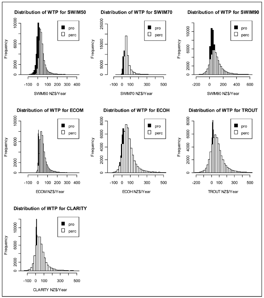
Comparing the mean and median WTP in Models 1 and 3 there is a clear indication that respondents in the SQ perceived model are more willing to pay for water quality improvements than those in the SQ provided model for all attributes. A similar trend is observed in Models 2 and 4 in which respondents with high income and qualification levels were excluded from the analysis. The median WTP values are less than the mean WTP values in both treatments for all attributes indicating that the distributions are highly skewed upwards. In general the differences in WTP values between the two treatments appear to be quite substantial. A graphical comparison of the distributions of WTP values across the two SQ treatments based on models estimated on all respondents (Model 1 and 3) are presented in Figure 1.
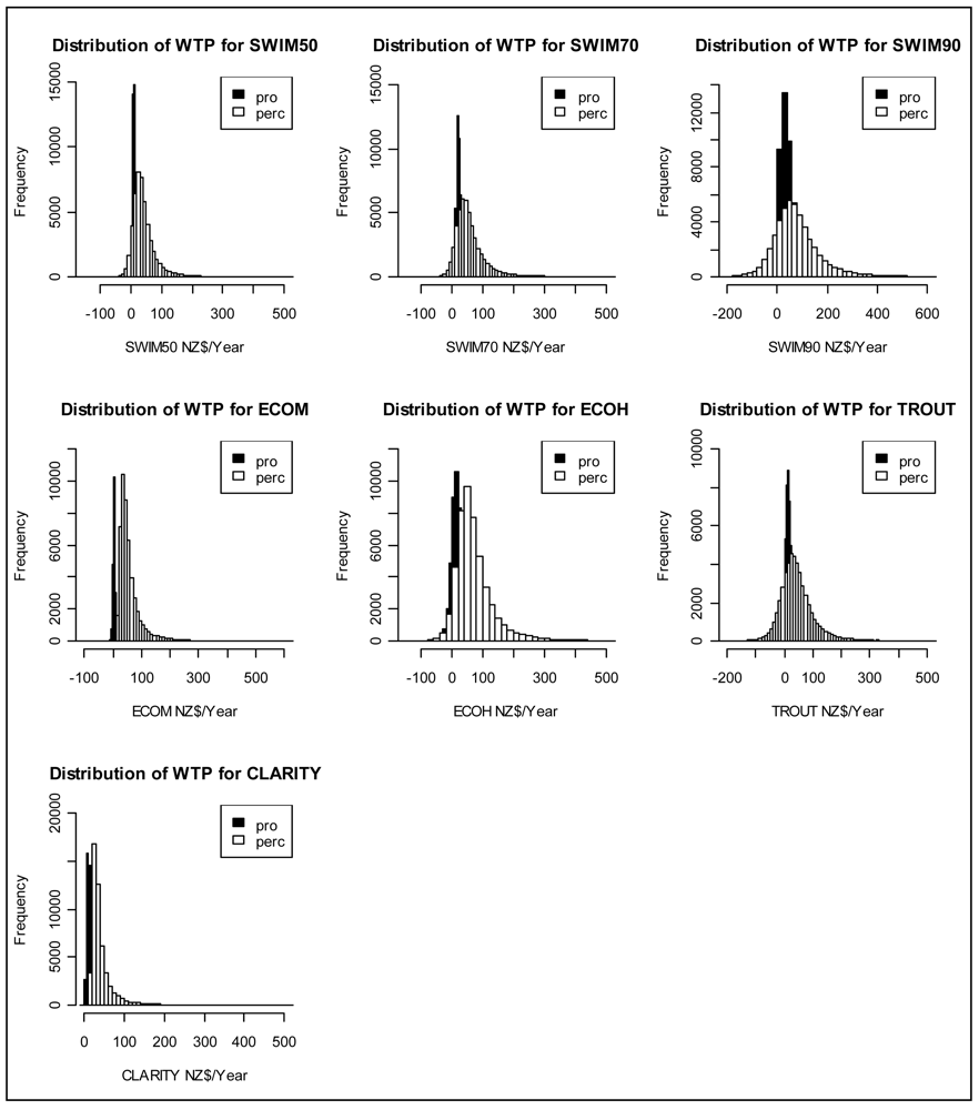
The distributions are highly skewed with long and fat tails towards the upper end of the scale. Further, analysis of the histograms highlights that although the distributions of the WTP for all attributes overlap, the WTP for most respondents in the SQ provided model is relatively lower than their counterpart. The Kolmogorov-Smirnov test (d-statistic) in Table 4 reveals that there are significant differences in WTP distributions for all attributes in the two treatments. Likewise, the simulated distributions of WTP for Model 2 and 4 are compared and presented in Figure 2 below:
Once more, the distributions are highly skewed with relatively fat tails towards the upper end of the scale, with the simulated population distribution of WTP from the SQ provided model being relatively lower than that from the SQ perceived model. The Kolmogorov-Smirnov test (d-statistic) again reveals that there are significant differences in the distributions of WTP values from the two subsamples (Table 4).
Our results suggest that the distributions of WTP values between the two treatments are significantly different. Poe et al. [62] states that:
“Differences in estimated WTP distributions do not necessarily imply that the means derived from these distributions are different. For instance, it is possible that two significantly different distributions can cross and have identical means.”
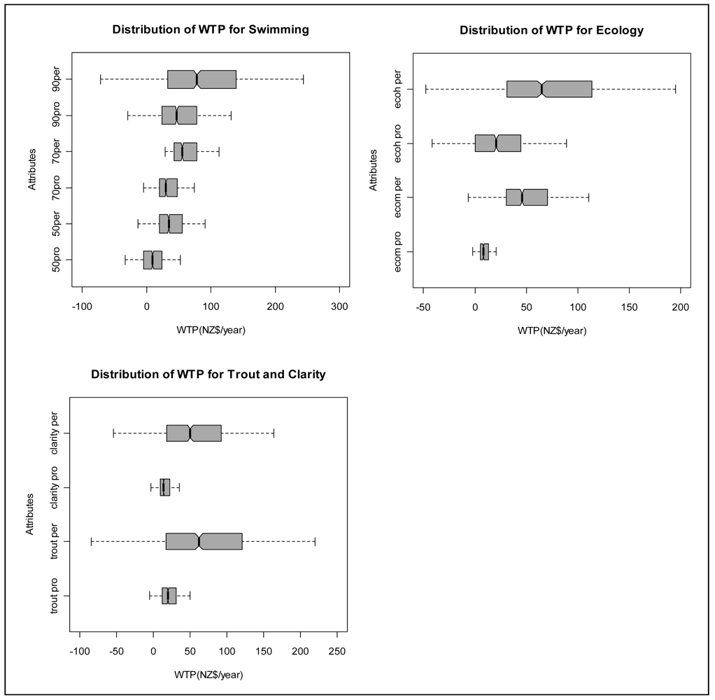
To graphically explore the differences in the simulated measures of central tendency between the two treatments, the quartiles of the distributions of WTP are compared using box plots see [63] and reported in Figures 3 and 4. The box plots display the upper and the lower limits of the cumulative distributions, and the inter-quartile range showing the first quartile, the median and the third quartile. Given that the distributions of WTP are highly skewed, the median is used as a basis of comparison as opposed to the mean, since the latter can be influenced by extreme values.
Figure 3 shows the box plots for Models 1 and 3 with all respondents included in the analysis.
The quartile distributions are consistent with the previous results, with respondents in the SQ perceived model generally showing higher WTP for all attributes than those in the SQ provided model. Specifically, the notches in the box plots signify the 95% confidence interval for the median. According to Chambers et al. [55], if the notches do not overlap, the null hypothesis of equal medians is rejected.
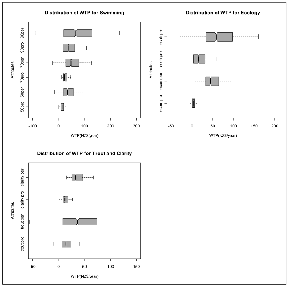
A similar comparison between the median WTP values for Models 2 and 4 in which respondents with high income and qualification levels were excluded from the analysis is presented in Figure 4 below:
Inspection of the box plots demonstrate that the notches do not overlap for all stream water quality attributes and therefore, the hypothesis of equal medians is rejected. This test is a further confirmation that respondents in the SQ perceived models display stronger preferences as implied by higher WTP values than those in the SQ provided models. The results further highlight that there is more variance in the WTP values in the SQ perceived models especially for SWIM90 (90 % of readings satisfactory for swimming), ECOH (excellent ecological health) and presence of trout, than in the SQ provided models.
6. Conclusions and Implications of the Study
The broader purpose of this research was to assess a community's preferences for stream water quality improvements. A specific focus in this paper was placed on the effect of accounting for perceived vs described status quo levels. The study revealed that about 58% of respondents had their own perceived baseline condition of water quality and that they could map it into the framework of attributes and levels proposed in the survey. On the other hand 41% of respondents were provided a SQ description by researchers because these respondents either had little or no prior knowledge of the prevailing conditions of water quality in streams or they had this knowledge but could not map it into the proposed framework. We believe that such a dichotomy is common in many nonmarket valuation studies, and hence its consequences for policy prescription via value estimation are worth exploring.
The results of our investigation show marked differences in the marginal value that these two groups of respondents place on water quality improvements and this has implications for their willingness to pay values. The respondents who were provided with status quo descriptions expressed strong preference for water that is suitable for swimming, has good clarity and where trout can be found. Yet, this group displayed a reluctance to stay with the SQ scenario. We argued that this might be the case because of their comparative ignorance of baseline water quality conditions. The second group of respondents, who adopted their own perceived SQ scenario, expressed significantly stronger preference for improvements across all the attributes subject of this study, but this tendency was attenuated by a general reluctance to embrace policy options implying changes from the SQ, about which they had quite good knowledge. For this group, estimates of marginal willingness to pay values are higher across the entire distribution than for respondents to whom the SQ information was provided.
Economic theory suggests that marginal WTP should be proportional to the expected improvement and this in turn depends on individual perceptions in one group and the provided description in the other. In our individual perception data we observe that on average perceived quality of the SQ conditions was higher than the one that was provided. This might be the cause for the observed reluctance to abandon the SQ, as manifested by a positive and significant alternative specific constant for the SQ alternative. In principle for this group the expected improvement would be perceived as smaller, and so would the associated marginal WTP when compared to that held by the SQ provided group. However, this holds only for quality changes within evaluations by the same respondent. Unfortunately this cannot be tested here because of the lack of a counterfactual.
The present study demonstrates the effects of using a coding specification of the status quo directly built on respondents' perceptions. Our results are supportive of the findings by Kataria et al. [22] which showed that failure to take account of respondents' beliefs leads to biased welfare estimates and earlier similar findings by Adamowicz et al. [20] in the context of integrating revealed preference data, in which the status quo was based on respondent's subjective perceptions, and stated preferences, where it was objectively described to them.


| Attribute | Current Situation | Improvement Levels | Labels | |||
|---|---|---|---|---|---|---|
| Suitability for Swimming (% of readings rated as satisfactory for swimming) | ASC | fixed SQ specific constant which is equal to 1 for the SQ and 0 for the other alternatives | ||||
| 30% | 50% | 70% | 90% | |||
| Variables | SWIM50 | SWIM70 | SWIM90 | |||
| Ecology (% of readings rated as excellent) | σε | error component capturing the extra variance associated with the experimentally designed alternatives. | ||||
| <40% Only small eels | 40–70% Small eels, bullies and smelt | >70% Large eels, bullies and smelt | ||||
| Variables | ECOM | ECOH | Per | denotes attributes pertaining to the SQ—perceived models | ||
| Trout | No Trout | Trout are found (TROUT) | Pro | denotes attributes pertaining to the SQ—provided models | ||
| Water Clarity | Usually you cannot see the bottom | Usually you can see the bottom (CLARITY) | ||||
| Cost to Household $ per year for the next 10 years (COST) | ||||||
| $0 | $50, $100, $200 | |||||
| Provided | Perceived | Sample | Region | |
|---|---|---|---|---|
| Gender (%) | ||||
| Males | 60 | 62 | 62 | 49 |
| Females | 40 | 38 | 38 | 51 |
| Age (%) | ||||
| Under 30 | 11 | 16 | 14 | 18 |
| 30–44 | 21 | 20 | 20 | 30 |
| 45–59 | 27 | 29 | 29 | 28 |
| 60+ | 40 | 34 | 37 | 25 |
| Education (%) | ||||
| Any post secondary qual. | 44 | 49 | 47 | |
| Vocational/trades | 19 | 21 | 16 | |
| Diploma or certificate (>1 year) | 19 | 37 | 24 | |
| Bachelors degree | 3 | 8 | 5 | |
| Higher degree | 1 | 4 | 2 | |
| Income (%) | ||||
| <$30,000 | 44 | 14 | 30 | 53 |
| $30 to $50,000 | 18 | 21 | 19 | 21 |
| $50 to $70,000 | 10 | 19 | 16 | 9 |
| $70 to $100, 000 | 12 | 20 | 13 | 4 |
| >$100,000 | 10 | 15 | 11 | 3 |
| Not revealed by respondent | 7 | 11 | 11 | 11 |
| Work on or own a farm (%) | 25 | |||
| Location (%) | ||||
| Town | 63 | 52 | 57 | |
| Settlement | 19 | 10 | 13 | |
| Rural | 4 | 16 | 11 | |
| Farm | 14 | 22 | 19 | |
| Sample Size | 73 | 103 | 178 |
| Model 1 SQ-Provided All Respondents | Model 2 SQ-Provided High Income & Qualification excluded | Model 3 SQ-Perceived All Respondents | Model 4 SQ-Perceived High Income & Qualification excluded | |||||
|---|---|---|---|---|---|---|---|---|
| Coefficient | |t-value| | Coefficient | |t-value| | Coefficient | |t-value| | Coefficient | |t-value| | |
| Variable | ||||||||
| ASC | −2.293 f | 5.04 | −2.143 f | 3.79 | 0.792 f | 2.19 | 0.550 f | 1.45 |
| SWIM50 | 0.344 r | 1.34 | 0.504 f | 1.74 | 0.601 f | 3.18 | 0.792 f | 3.04 |
| SWIM70 | 1.130 f | 4.45 | 1.020 f | 3.28 | 0.954 f | 4.65 | 1.103 f | 3.99 |
| SWIM90 | 1.641 r | 5.07 | 1.510 f | 4.25 | 1.281 r | 5.17 | 1.765 r | 4.71 |
| ECOM | 0.301 f | 1.47 | 0.131 r | 0.53 | 0.829 f | 4.83 | 0.954 f | 3.98 |
| ECOH | 0.602 r | 2.27 | 0.687 r | 2.21 | 1.187 r | 5.59 | 1.438 r | 4.77 |
| TROUT | 0.711 f | 3.84 | 0.636 f | 2.91 | 1.014 r | 5.12 | 0.834 r | 3.18 |
| CLARITY | 0.507 f | 2.65 | 0.532 f | 2.35 | 0.820 r | 5.14 | 0.835 f | 4.06 |
| COST | −0.035 r | 5.04 | −0.041 r | 6.75 | −0.017 r | 8.59 | −0.023 r | 6.04 |
| Error Component | 2.692 | 6.91 | 2.487 | 5.93 | 3.341 | 7.22 | 2.181 | 5.86 |
| σε | ||||||||
| Summary Statistics | ||||||||
| Log L | −513.6 | −342.7 | −742.2 | −387.3 | ||||
| AIC | 1.202 | 1.206 | 1.223 | 1.213 | ||||
| BIC | 1.273 | 1.296 | 1.282 | 1.301 | ||||
| R2 (McFadden) | 0.466 | 0.469 | 0.453 | 0.466 | ||||
| N (Observations) | 876 | 588 | 1236 | 660 | ||||
Note:f and rdenote whether the attributes were estimated as fixed or random variables.
| Attribute | Model 1 SQ-Provided | Model 3 SQ-Perceived | d-stat' | Model 2 SQ-Provided | Model 4 SQ-Perceived | d-stat' | ||||
|---|---|---|---|---|---|---|---|---|---|---|
| All Respondents | All Respondents | High Income & Qualification Excluded | ||||||||
| Mean | Median | Mean | Median | Mean | Median | Mean | Median | |||
| SWIM50 | 13.4 | 9.56 | 48.4 | 34.82 | 0.455 | 17.63 | 12.64 | 48.28 | 34.7 | 0.524 |
| SWIM70 | 42.59 | 30.72 | 77.65 | 55.86 | 0.505 | 32.01 | 22.99 | 67.21 | 48.34 | 0.447 |
| SWIM90 | 67.19 | 48.05 | 109.05 | 78.67 | 0.249 | 51.97 | 37.24 | 92.89 | 66.765 | 0.281 |
| ECOM | 11.74 | 8.47 | 64.41 | 46.33 | 0.780 | 4.92 | 3.52 | 63.98 | 46.15 | 0.941 |
| ECOH | 30.29 | 21.71 | 91.01 | 65.61 | 0.408 | 23.83 | 17.07 | 83.85 | 60.28 | 0.529 |
| TROUT | 27.69 | 19.95 | 85.46 | 61.79 | 0.475 | 19.91 | 14.26 | 51.39 | 36.93 | 0.398 |
| CLARITY | 19.75 | 14.15 | 69.3 | 49.99 | 0.526 | 16.52 | 11.84 | 45.99 | 33.16 | 0.745 |
All d-statistics have significance at p-value < 0.001.
Acknowledgments
This research was carried out under FRST Programme C10X0603: Delivering tools for improved environmental performance funded by The Foundation for Research Science and Technology (FRST) and the Pastoral 21 partners Dairy New Zealand, Meat and Wool New Zealand and Fonterra.
References and Notes
- Gravitas Research and Strategy Ltd. Environmental Awareness, Attitudes and Actions, 2006: A Survey of Residents of the Waikato Region; Environment Waikato: Hamilton, ON, Canada, 2007. [Google Scholar]
- Ministry for the Environment. Environment New Zealand 2007; Ministry for the Environment: Wellington, New Zealand, 2008. [Google Scholar]
- Environment Waikato. Best Management Practices. Improving Nutrient Efficiency; Environment Waikato: Hamilton, New Zealand; 27; August; 2009. [Google Scholar]
- Louviere, J.; Hensher, D.A. Design and analysis of simulated choice or allocation experiments in travel choice modeling. Transp. Res. Rec. 1982, 890, 11–17. [Google Scholar]
- Louviere, J.; Woodworth, G. Design and analysis of simulated consumer choice or allocation experiments: An approach based on aggregate data. J. Mark. Res. 1983, 20, 350–367. [Google Scholar]
- Boxall, P.; Adamowicz, W.; Swait, J.; Williams, M.; Louviere, J. A comparison of stated preference methods for environmental valuation. Ecol. Econ. 1996, 18, 243–253. [Google Scholar]
- Adamowicz, W.; Boxall, P.; Williams, M.; Louviere, J. Stated preference approaches for measuring passive use values: Choice experiments and contingent valuation. Am. J. Agric. Econ. 1998, 80, 64–75. [Google Scholar]
- Brazell, J.D.; Diener, C.G.; Karniouchina, E.; Moore, W.L.; Séverin, V.; Uldry, P. The no-choice option and dual response choice designs. Mark. Lett. 2006, 17, 255–268. [Google Scholar]
- Boxall, P.; Adamowicz, W.L.; Moon, A. Complexity in choice experiments: Choice of the status quo alternative and implications for welfare measurement*. Aust. J. Agric. Resour. Econ. 2009, 53, 503–519. [Google Scholar]
- Breffle, W.S.; Rowe, R.D. Comparing choice question formats for evaluating natural resource tradeoffs. Land Econ. 2002, 78, 298–314. [Google Scholar]
- Dhar, R.; Simonson, I. The effect of forced choice on choice. J. Mark. Res. 2003, 40, 146–160. [Google Scholar]
- Scarpa, R.; Ferrini, S.; Willis, K. Performance of Error Component Models for Status-Quo Effects in Choice Experiments. In Applications of Simulation Methods in Environmental and Resource Economics; Scarpa, R., Alberini, A., Eds.; Kluwer Acadenic Publishers: London, UK, 2005. [Google Scholar]
- Hess, S.; Rose, J.M. Should reference alternatives in pivot design SC surveys be treated differently? Environ. Resour. Econ. 2009, 42, 297–317. [Google Scholar]
- Rose, J.M.; Bliemer, M.C.J.; Hensher, D.A.; Collins, A.T. Designing efficient stated choice experiments in the presence of reference alternatives. Transp. Res. Part B 2008, 42, 395–406. [Google Scholar]
- Campbell, D.; Hutchinson, W.G.; Scarpa, R. Incorporating discontinuous preferences into the analysis of discrete choice experiments. Environ. Resour. Econ. 2008, 41, 401–417. [Google Scholar]
- Rose, J.M.; Scarpa, R. Design efficiency for nonmarket valuation with choice modelling: How to measure it, What to report and why. Aust. J. Agric. Resour. Econ. 2008, 52, 253–282. [Google Scholar]
- Morrison, M.; Bennett, J. Valuing New South Wales rivers for use in benefit transfer. Aust. J. Agric. Resour. Econ. 2004, 48, 591–611. [Google Scholar]
- Kragt, M.E.; Bennett, J.W. Using Choice Experiments to Value River and Estuary Health in Tasmania with Individual Preference Heterogeneity. Proceedings of the 53rd Annual Conference-Australian Agricultural and Resource Economics Society, Cairns, Australia, 10–13 February 2009.
- Adamowicz, W.; Louviere, J.; Swait, J. Introduction to Attribute-Based Stated Choice Methods.; Final report; National Oceanic and Atmospheric Administration (NOAA): Washington, DC, USA, 1998. [Google Scholar]
- Adamowicz, W.; Swait, J.; Boxall, P.; Louviere, J.; Williams, M. Perceptions versus objective measures of environmental quality in combined revealed and stated preference models of environmental valuation. J. Environ. Econ. Manag. 1997, 32, 65–84. [Google Scholar]
- Barton, D.N.; Navrud, S.; Lande, N.; Mills, A.B. Assessing Economic Benefits of Good Ecological Status in Lakes under the EU Water Framework Directive; NIVA Report 5732-2009; Norwegian Institute for Water Research (NIVA), Norwegian University of Life Sciences (UMB): Oslo, Norway, 2009. [Google Scholar]
- Kataria, M.; Ellingson, L.; Hasler, B.; Nissen, C.; Christensen, T.; Martinsen, L.; Ladenburg, J.; Levin, G.; Dubgaard, A.; Bateman, I.; Hime, S. Scenario Realism and Welfare Estimates in Choice Experiments: Evidence from a Study on Implementation of the European Water Framework Directive in Denmark. Proceedings of the 17th Annual Conference of the European Association of Environmental and Resource Economists, Amsterdam, The Netherlands, 24–27 June 2009.
- Glenk, K. Using local knowledge to model asymmetric preference formation in willingness to pay for environmental services. J. Environ. Manag. 2011, 92, 531–541. [Google Scholar]
- Ortúzar, J.D.; Willumsen, L.G. Modelling Transport, 3rd ed.; John Wiley and Sons: Chichester, UK, 2001. [Google Scholar]
- Starmer, C. Developments in non-expected utility theory: The hunt for a descriptive theory of choice under risk. J. Econ. Lit. 2000, 38, 332–382. [Google Scholar]
- Kahneman, D.; Tversky, A. Prospect Theory: An analysis of decisions under risk. Econometrica 1979, 47, 263–291. [Google Scholar]
- Gilboa, I.; Schmeidler, D.; Wakker, P.P. Utility in case-based decision theory. J. Econ. Theory 2002, 105, 483–502. [Google Scholar]
- Adamowicz, V.; Boxall, P. Future Directions of Stated Choice Methods for Environment Valuation. In Paper Prepared for: Choice Experiments: A New Approach to Environmental Valuation; London, UK, 2001. [Google Scholar]
- Hensher, D.A.; Jones, S.; Greene, W.H. An error component logit analysis of corporate bankruptcy and insolvency risk in Australia. Econ. Rec. 2007, 83, 86–103. [Google Scholar]
- Kahneman, D.; Knetsch, J.L.; Thaler, R.H. Anolmalies: The endownment effect, loss aversion and status quo bias. J. Econ. Perspect. 1991, 5, 193–206. [Google Scholar]
- Samuelson, W.; Zeckhauser, R. Status quo bias in decision making. J. Risk Uncertain. 1988, 1, 7–59. [Google Scholar]
- Bateman, I.; Munro, A.; Rhodes, B.; Starmer, C.; Sugden, R. A test of the theory of reference-dependent preferences. Q. J. Econ. 1997, 112, 479–505. [Google Scholar]
- Kahneman, D.; Tversky, A. Prospect theory: An analysis of decision under risk. Econometrica 1979, 47, 263–292. [Google Scholar]
- Adamowicz, W.; Dupont, D.; Krupnick, A.; Zhang, J. Valuation of cancer and microbial disease risk reductions in municipal drinking water: An analysis of risk context using multiple valuation methods. J. Environ. Econ. Manag. 2011, 61, 213–226. [Google Scholar]
- Meyerhoff, J.; Liebe, U. Status quo effect in choice experiments: Empirical evidence on attitudes and choice task complexity. Land Econ. 2009, 85, 515–528. [Google Scholar]
- Boxall, P.; Adamowicz, W.L.V.; Moon, A. Complexity in choice experiments: Choice of the status quo alternative and implications for welfare measurement. Aust. J. Agric. Resour. Econ. 2009, 53, 503–519. [Google Scholar]
- Lehtonen, E.; Kuuluvainen, J.; Pouta, E.; Rekola, M.; Li, C.-Z. Non-market benefits of forest conservation in southern Finland. Environ. Sci. Policy 2003, 6, 195–204. [Google Scholar]
- Li, C.-Z.; Kuuluvainen, J.; Pouta, E.; Rekola, M.; Tahvonen, O. Using choice experiments to value the natura 2000 nature conservation programs in Finland. Environ. Resour. Econ. 2004, 29, 361–374. [Google Scholar]
- Scarpa, R.; Campbell, D.; Hutchinson, W.G. Benefit estimates for land improvements: Sequential bayesian design amd respondents' rationality in a choice experiment. Land Econ. 2007b, 83, 617–634. [Google Scholar]
- Scarpa, R.; Willis, K.G.; Acutt, M. Valuing externalities from water supply: Status quo, choice complexity and individual random effects in panel kernel logit analysis of choice experiments. J. Envrion. Plan. Manag. 2007a, 50, 449–466. [Google Scholar]
- Scarpa, R.; Thiene, M.; Marangon, F. Using flexible taste distributions to value collective reputation for environmentally friendly production methods. Can. J. Agric. Econ. 2008, 56, 145–162. [Google Scholar]
- Ferrini, S.; Scarpa, R. Designs with a priori information for nonmarket valuation with choice experiments: A monte carlo study. J. Environ. Econ. Manag. 2007, 53, 342–363. [Google Scholar]
- Hu, W.; Boehle, K.; Cox, L.; Pan, M. Economic values of Dolphin Excursion in Hawaii: A stated analysis. Mar. Resour. Econ. 2009, 24, 61–76. [Google Scholar]
- Scarpa, R.; Ferrini, S.; Willis, K. Performance of Error Component Models for Status-Quo Effects in Choice Experiments. In Applications of Simulation Methods in Environmental and Resource Economics; Springer Netherlands: Dordrecht, The Netherlands, 2005; Volume 6, pp. 247–273. [Google Scholar]
- Train, K. Discrete Choice Methods with Simulation; Cambridge University Press: Cambridge, UK, 2003. [Google Scholar]
- Banzhaf, M.R.; Johnson, F.R.; Mathews, K.E. Opt-Out Alternatives and Anglers' Stated Preferences. In The Choice Modelling Approach to Environmental Valuation; Bennett, J., Blamey, R., Eds.; Edward Elgar: London, UK, 2001; pp. 157–177. [Google Scholar]
- Revelt, D.; Train, K. Mixed logit with repeated choices: Households' choices of appliance efficiency level. Rev. Econ. Stat. 1998, 80, 647–657. [Google Scholar]
- Train, K.E. Recreation demand models with taste differences over people. Land Econ. 1998, 74, 230–239. [Google Scholar]
- Herriges, J.A.; Phaneuf, D.J. Inducing patterns of correlation and substitution in repeated logit models of recreation demand. Am. J. Agric. Econ. 2002, 84, 1076–1090. [Google Scholar]
- Brownstone, D.; Train, K. Forecasting new product penetration with flexible substitution patterns. J. Econ. 1999, 89, 109–129. [Google Scholar]
- Ben-Akiva, M.; Bolduc, D.; Walker, J. Specification, identification and estimation of the logit kernel (or continuous mixed logit) model; February; 2001; unpublished. [Google Scholar]
- Hensher, D.A.; Rose, J.M.; Greene, W.H. Applied Choice Analysis; Cambridge University Press: Cambridge, UK, 2005. [Google Scholar]
- Hensher, D.; Greene, W. The Mixed logit model: The state of practice. Transportation 2003, 30, 133–176. [Google Scholar]
- Thiene, M.; Scarpa, R. Deriving and testing efficient estimates of WTP distributions in destination choice models. Environ. Resour. Econ. 2009, 44, 379–395. [Google Scholar]
- Chambers, J.; William, C.; Beat, K.; Paul, T. Graphical Methods for Data Analysis; Wadsworth Publishing: Stamford, CT, USA, 1983. [Google Scholar]
- Krueger, R.A. Focus Groups. A Practical Guide for Applied Research; SAGE: Thousand Oaks, CA, USA, 1994. [Google Scholar]
- Bell, B.; Yap, M. The Rotorua Lakes. Evaluation of Less Tangible Values; Nimmo-Bell & Company: Wellington, New Zealand, 2004. [Google Scholar]
- Kerr, G.N.; Swaffield, S.R. Amenity Values of Spring Fed Streams and Rivers in Canterbury, New Zealand: A Methodological Exploration. In Research report, No. 298.; Lincoln University, Agribusiness and Economics Research Unit: Canterbury, New Zealand; November; 2007. [Google Scholar]
- Environment Waikato Stream and River Life. Available online: http://www.ew.govt.nz/Environmental-information/Rivers-lakes-and-wetlands/healthyrivers/Stream-and-river-life/ (accessed on 7 September 2011).
- Joy, M. A Predictive Model of Fish Distribution and Index of Biotic Integrity (IBI) for Wadeable Streams in the Waikato Region; Environment Waikato: Hamilton, ON, Canada, 2005. [Google Scholar]
- Loomes, G.; Sugden, R. Regret theory: An alternative theory of rational choice under uncertainty. Econ. J. 1982, 92, 805–824. [Google Scholar]
- Poe, G.L.; Severance-Lossin, E.K.; Welsh, M.P. Measuring the difference (X-Y) of simulated distributions: A convolutions approach. Am. J. Agric. Econ. 1994, 76, 904–915. [Google Scholar]
- Tukey, J. Exploratory Data Analysis; Addison-Wesley: Boston, MA, USA, 1977. [Google Scholar]
© 2011 by the authors; licensee MDPI, Basel, Switzerland. This article is an open access article distributed under the terms and conditions of the Creative Commons Attribution license (http://creativecommons.org/licenses/by/3.0/).
Share and Cite
Marsh, D.; Mkwara, L.; Scarpa, R. Do Respondents’ Perceptions of the Status Quo Matter in Non-Market Valuation with Choice Experiments? An Application to New Zealand Freshwater Streams. Sustainability 2011, 3, 1593-1615. https://doi.org/10.3390/su3091593
Marsh D, Mkwara L, Scarpa R. Do Respondents’ Perceptions of the Status Quo Matter in Non-Market Valuation with Choice Experiments? An Application to New Zealand Freshwater Streams. Sustainability. 2011; 3(9):1593-1615. https://doi.org/10.3390/su3091593
Chicago/Turabian StyleMarsh, Dan, Lena Mkwara, and Riccardo Scarpa. 2011. "Do Respondents’ Perceptions of the Status Quo Matter in Non-Market Valuation with Choice Experiments? An Application to New Zealand Freshwater Streams" Sustainability 3, no. 9: 1593-1615. https://doi.org/10.3390/su3091593
APA StyleMarsh, D., Mkwara, L., & Scarpa, R. (2011). Do Respondents’ Perceptions of the Status Quo Matter in Non-Market Valuation with Choice Experiments? An Application to New Zealand Freshwater Streams. Sustainability, 3(9), 1593-1615. https://doi.org/10.3390/su3091593