A Carbon Consumption Comparison of Rural and Urban Lifestyles

Abstract
: Sustainable consumption has been addressed from different perspectives in numerous studies. Recently, urban structure-related lifestyle issues have gained more emphasis in the research as cities search for effective strategies to reduce their 80% share of the global carbon emissions. However, the prevailing belief often seen is that cities would be more sustainable in nature compared to surrounding suburban and rural areas. This paper will illustrate, by studying four different urban structure related lifestyles in Finland, that the situation might be reversed. Actually, substantially more carbon emissions seem to be caused on a per capita level in cities than in suburban and rural areas. This is mainly due to the higher income level in larger urban centers, but even housing-related emissions seem to favor less urbanized areas. The method of the study is a consumption-based life cycle assessment of carbon emissions. In more detail, a hybrid life cycle assessment (LCA) model, that is comprehensive in providing a full inventory and can accommodate process data, is utilized.1. Introduction
Cities have been both blamed for climate change [1,2] and defended [3] in comparison to rural and semi-urban areas. The per capita carbon emissions in cities have been reported as substantially lower than those of the surrounding rural and suburban areas and the country average in several studies [4-6]. In addition, high density areas, based on multi-storey buildings, have been reported to cause significantly less carbon emissions on a per capita basis than low-density low-rise areas [7]. However, almost completely opposite results have been reported recently [8].
Unquestionably, the importance of cities in the search for effective climate change mitigation strategies is high, as cities have been estimated to produce up to 80% of global greenhouse gases (GHGs) [9]. However, the approaches utilized in a vast majority of earlier studies are not sufficient to conclude cities or rural areas as more sustainable in preventing climate change. The approaches have two notable deficiencies. First, they have concentrated on the producer perspective, allocating the GHG emissions for a city or region that can occur inside the borders of the region. This seems to favor cities as heavy industries and energy production are often located outside of the city borders. Second, a relevant question left unanswered in them, is how the type of a region, city or rural, affects the consumption habits, i.e., the lifestyle. If cities accommodate more consumption-intensive lifestyles, the possible advantage of high density and dwelling-based housing might easily be lost in comprehensive carbon emission calculations.
This paper presents an empirical consumption-based assessment of the carbon emissions caused by consumers living in different types of communities. We utilize the life cycle assessment (LCA) method to assess the GHGs (CO2, CH4, N2O and HFC/PFCs) attributable to private consumption. This approach enables global comparisons as no regional borders need to be set. Also, the approach allows an analysis of the relations between consumption habits and the area or habitation type.
The study utilizes urbanization rate-based samples from rural to metropolitan areas taken from a large consumer survey representing different consumer profiles in Northern Europe. The consumer profiles offer a possibility to assess the carbon consumption, the GHG emission associated with consumption of commodities in carbon equivalents, related to the lifestyles in different area types.
In the paper we will demonstrate that, when a change from rural to urban area type leads to upgrade in the income level, and thus in the consumption volume, urbanization might lead to significantly higher carbon emissions instead of diminishing of the emissions. We argue that this perspective will be of high importance in the future in the search for effective climate change mitigation strategies. Together with the more common regional production-based assessments, the two perspectives provide sustainable basis for strategic decision making in an urban development.
2. Method
The study is conducted utilizing the LCA method. The method includes two main approaches: input-output-LCA (IO-LCA), process-LCA, and a combination of the two, namely hybrid-LCA. The three approaches together with the main solutions are shortly presented below.
The traditional way of conducting an LCA, process-LCA, assesses the emissions based on energy and mass flows in the production and supply chain processes inside the selected assessment boundaries [10-12]. The accurateness of the method is potentially very high as the emissions are measured as they are generated. However, even by including multiple upstream processes into the assessments, the approach suffers from truncation error from the boundary selection that always needs to be made. The amount of processes that add emissions to a certain good or service is normally very high if all production and supply chain processes are calculated. These boundary selection-based cutoffs may potentially significantly affect the result of the assessment [10]. Also, a comprehensive process-LCA is inherently laborious and time consuming to conduct [10,11] due to the described nature of the assessment.
IO-LCA, in turn, assesses the emissions based on monetary transactions, the basic idea being that every monetary transaction is related to production of a good or service that causes emissions [11]. The IO method is based on transaction tables that describe the connections between different industries, normally within a certain national economy [12]. The tables show the emissions that each sector causes related to a monetary transaction on one sector. The tables capture both the energy and non-energy related GHG emissions from each industry sector in the supply chain related to production and distribution of a product over its lifetime, thus including the embedded as well as the production phase emissions. Together these form a comprehensive carbon footprint of a certain good or service independent of the geographic place where the production or the consumption occurs. The carbon footprint referred in this paper is thus in accordance with several definitions, i.e., Pandey et al. (2010) [13].
The IO method does not suffer from the truncation error described above. The method is comprehensive, always providing a full inventory of the emissions attributable to a certain good [11,14], except for the end of life stage, which should be added to the calculations [10]. Input output method is also quick and rather easy to use [11].
There are three types of inherent problems related to IO method. The first is a high level of aggregation of industry classifications. Even in the most disaggregated model, the number of industry sectors is less than 500 [15], significantly lower than in an economy in reality. The second include possible temporal (inflation and currency rate differences) and regional (industry structure differences) asymmetries between the data and the model. The models available are not updated annually, and the industry structure of the model might deviate from that of the region studied. Third, the models generally assume domestic production of imports, meaning that the emissions intensities are always the same for each sector [10,11,16].
Although both of the described approaches have weaknesses, the inherent problems differ from each other. This creates space for the approach combining the strengths of the two approaches and reducing the weaknesses related to them; hybrid-LCAs [10,17]. The hybrid-LCA method allows life cycle assessments with lacking information, and enables creation of models that significantly reduce the truncation error inherent in process-LCAs while reaching to process specificity. In addition, hybrid-LCAs suit well for assessments within the context of the built environment, where the studied systems tend to be complex in nature [18]. Three different approaches can be distinguished in hybrid-LCAs: tiered hybrid LCA, IO-based hybrid analysis and integrated hybrid analysis [10].
In this study we exploit an IO-based application of tiered hybrid-LCA, utilized also earlier by Heinonen and Junnila [8], to assess the GHGs related to private consumption. The model retains the comprehensiveness of IO approach while reaching for the accurateness of a process approach. The model is based on IO tables to maintain full coverage of the inventory. To increase the accuracy, the key emission sources are assessed with local process data. The utilized model and its construction is further described in the next section.
3. Research design
3.1. Rural, Semi-Urban, City and Metropolitan Consumers
Four representative samples of consumers from Finland were selected for the study covering a range of types of living from rural to metropolitan to assess the carbon consumption of an average consumer of each living type.
The first sample consists of consumers living in Finnish rural regions. These consist of regions where less than 60% of the inhabitants live in urban areas with the largest urbanization smaller than 15,000 inhabitants, or of regions where 60 to 90% of the inhabitants live in urban areas with a maximum of 4,000 inhabitants. The second sample, the semi-urban regions, comprises consumers from municipalities where 60 to 90% of the inhabitants live in urban areas with 4,000–15,000 inhabitants. The third sample, the cities, consists of consumers of municipalities where a minimum of 90% of the inhabitants live in urban areas, and those where the largest urbanization is larger than 15,000 inhabitants. The Helsinki metropolitan area forms the fourth sample. The region consists of the capital of Finland, Helsinki, and the three large cities surrounding Helsinki, the region together having around 1,000,000 inhabitants. In addition, the Finnish average carbon consumption was assessed to support the analysis.
The described selection of lifestyle-based samples enabled us to demonstrate the changes in carbon consumption from three perspectives: growth of the urban density, change in the dominant type of habitation from detached houses to apartment buildings, and growth in the income level. In rural areas, detached housing is dominating and the areal structures are loose. On the other end, in the Helsinki metropolitan area, the urban structure is substantially denser and apartment buildings dominate housing. Semi-urban areas and cities fall between the two extremes. In addition, the differences in the income levels and the consumption volumes are significant. In rural areas the annual consumption volume an average consumer is 12,200 € whereas that of an average consumer in the Helsinki metropolitan area is 17,600 €. Again, semi-urban areas and cities fall between these values [19]. Table 1 gathers together the important figures related to the four samples.
3.2. Input Data
The four samples forming the exploited input data were taken from the Finnish consumer survey 2006 [19]. The consumer survey 2006 data describes the consumption of an average Finnish consumer. The survey presents the consumption of an average consumer in very detailed form as it includes around 1,000 categories and sub-categories of goods and services. The sample size, nearly 10,000 participants on a national level (0.2% of the Finnish population), can also be considered representative. Smaller samples can be produced based on diverse variables, type of areal structure and region being the ones used in this study. This survey data were used as inputs in the carbon consumption assessments of the study.
The utilized process data include the average Finnish emissions of heat and electricity production, fuel combustion emissions of private driving and public transport, disaggregation of the public transport sector according to the local profiles of public transport use, and a regional price level correction on property prices. The data are described in more detail in the next section.
3.3. Tiered Hybrid-LCA Model
The study consists of two calculation phases, a direct IO assessment and a hybrid assessment. For the calculations, the original 1,000 categories were aggregated down to 43 consumption sectors representing the region and lifestyle-related consumption. After this, two different assessment models were utilized to calculate the carbon consumption of an average Finn: the Carnegie-Mellon EIO-LCA US Industry benchmark 2002 based model [15] as the primary model, and the Finnish ENVIMAT [20] to evaluate the result. The Finnish average consumption volumes in the above-mentioned 43 consumption sectors were utilized as inputs for both models. The overall results of the two assessments were very similar, within a 5% range of each other, supporting the use of the Carnegie Mellon EIO-LCA as the basis of our hybrid model. The EIO-LCA output matrices are publicly available, which enables construction of tiered hybrid applications. The emissions included in the model are CO2, CH4, N2O and HFC/PFCs calculated in carbon equivalents (100 years equivalency). Furthermore, the model is the most disaggregated model available, providing output tables for 428 industry sectors, reducing thus the aggregation error inherent in IO approaches. This was given high importance as the input data utilized in the study is highly complex. The problem of high level of aggregation of the industry sectors, inherent in all IO models, has been addressed by a number of studies. Of these, Lenzen et al. (2004) state that the level of disaggregation has significant impact on the results and thus the most disaggregated model should be utilized [21]. The Finnish economy is also a small and open economy with over 50% of the value of total consumption oriented to import goods [22], a significant part of the emissions attributable to Finnish consumption thus originating abroad. Of the model dimensions, the first tier utilized to accommodate local process data, the production or combustion phase, complies the WRI (2009) [23] Scopes 1 and 2 definitions. The whole model, in turn, is in accordance with the Scope 3 definition.
The model selection includes some potential sources of bias in addition to those inherent for the IO approach in general. First, as in all IO-based LCA assessments, the number of included processes is infinite within the system boundary defined by the scope of the model [10]. However, the problem that arises is an assumption of domestic production of imports. In this study, this means US industry emissions intensities for all the commodities outside of the utilized Finnish process data. The potential industry structure and emissions asymmetry error between a US based model and Finnish consumption profiles was assessed as not very significant according to the comparative assessment with the ENVIMAT model. Larsen and Hertwich (2009) also employ the same type of EIO-LCA based tiered hybrid LCA model in their study concerning the public sector in Norway arguing for the suitability of EIO-LCA in a similar northern country context [24]. However, Weber and Matthews (2008) report a 15% increase in the US household carbon emissions when the international trade is explicitly modeled [25]. This uncertainty is further discussed later in the paper.
Second, to decrease the temporal asymmetry problem arising from inflation and currency rate differences between the US and the Finnish economies, and the base years of the model and the input data, the model was adjusted with purchasing power parity (PPP) multiplier [26], a method that was utilized by Weber and Matthews in their fairly recent study of the global and distributional aspects of the American household carbon footprint [16].
Third, as inherent in all IO-based models, the output tables exclude the emissions from the use and the end of life phases. However, the use of total private consumption as the input data reduces this problem significantly. The costs related to these phases are embedded either in the consumer prices of goods and services or included in the input data as waste and recycling costs.
The final problem that needs to be assessed in IO method-based calculations is the accuracy problem arising from the use of the use of industry averages in the output matrices. In this study, the use of a hybrid assessment model reduces this problem as the utilization of the US industry averages can be avoided. The sectors enhanced with local process data cover more than 50% of the total carbon emissions, and all the most significant emission sources, as is further described below.
In the second phase the direct IO assessment was used for the design of the tiered hybrid-LCA model. In the tiered hybrid-LCA the most important processes creating carbon emissions according to the IO model were enhanced with local process data, but the rest of each output matrix, the EIO-LCA result matrices describing the emissions of each industry sector related to a monetary transaction on a certain sector, was left untouched to maintain the full coverage of the model.
In the direct IO assessment, four sectors were found to cover two thirds of the carbon consumption in all the samples. These four sectors were emissions related to housing energy use (heat and electricity), building related emissions and transport-related emissions divided into public transport and private driving. According to this assessment these four key sectors were enhanced with process data.
Concerning housing energy, the production phase emissions, the first tier in the output matrix, were replaced with process data. We utilized the average Finnish emission profiles for electricity, district heat and oil assessed with energy method, that allocates the production phase emissions of combined heat and electricity production directly according to the distribution of the total production between the two. According to Kurnitski and Keto [27] the carbon intensities in Finland are 240 g CO2/kWh for electricity, 286 g CO2/kWh for district heat and 267 g CO2/kWh for oil. For private use of firewood, zero carbon emissions were assumed. The Finnish electric power production profile behind the figures is: nuclear power 28%, fossil fuels 36%, peat 8% and renewable energy sources 28%.
The consumption survey, the input data, distinguishes in detail the maintenance charges of privately owned detached houses, but the maintenance paid as housing management charges or rents are embedded within these costs. To increase the reliability of the assessment, the communal building energy, normally paid with rent or housing management charges in apartment buildings and row-houses, was added to the energy consumption of a consumer by disaggregating the consumption sectors of housing management charges and rents. The average shares of communal heat and electricity attributable to each inhabitant were calculated in a study including eight housing corporations from the Helsinki metropolitan area [28]. Furthermore, all the other operation and maintenance costs included in rents and housing management charges, water, waste, cleaning, maintenance and repair construction, etc., were re-allocated under appropriate consumption categories according to the results of Kiiras et al. [29].
In private driving, the first tier emissions, the direct emissions from fuel combustion, were also replaced with process data. The process data utilized was taken from The Technological Centre of Finland's LIPASTO study, the emissions per passenger kilometer (pkm) being 179 g CO2-eqv. [30].
Next, the emissions from expenditure on building and property were enhanced with regional data. These expenditures are separated from the management costs in the input data, except of the share embedded in the rental payments. The embedded share was distinguished from the rental payments by assuming that the division of the costs between management charges and payments of building and property is similar to the privately owned apartments. Of these, the share of the price of property has substantial regional variations, and as the emissions related to building and property differ heavily, regional price adjustments were utilized according to the property price statistics of The Housing Finance and Development Centre of Finland (ARA) [31]. After the adjustment, the building share of the expenditure was allocated to construction of residential buildings, whereas the emissions related to the property were assessed with a low-intensity office work sector.
Finally, while emissions related to public transport had minor significance in the IO calculation, they were enhanced with Finnish industry-based data as the sector forms an important substitute for private driving, and the emissions profile of EIO-LCA significantly differs from that of Finland. The enhancement method was full replacement of the EIO-LCA output matrix with that of the respective Finnish ENVIMAT study.
After the construction of the hybrid model, we further combined the 43 consumption categories down to 10 consumption areas, which indicate the type of region and income level-related carbon consumption. The utilized consumption areas are:
Heat and electricity;
Building and property;
Maintenance and operation;
Private driving;
Public transportation;
Consumer goods;
Leisure goods;
Leisure services;
Travelling abroad;
Health, nursing and training services.
Of the 10 consumption areas, Heat and electricity contain all housing energy use, including both household heat and electricity and the share of communal building energy. Building and property is dominated by construction, whereas Maintenance and operation comprise emissions of maintenance and repair construction, water and waste water, waste and cleaning. Private driving, in addition to gasoline combustion, includes all activities related to driving, purchases and maintenance of private vehicles. Public transportation mostly consists of travelling by coach or train.
Goods and services classes comprise daily consumption and consumption of durable goods, so that leisure-related expenses are separated for demonstration of the allocation of emissions and lifestyle differences. Travelling abroad include all private flying and accommodation abroad. Finally, health, nursing and training services are put together as they only include private services, which in Finland form a minor share of all the services of these sectors.
4. Results
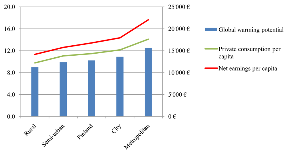
The study produced an unconventional but really interesting outcome. The results indicate that the level of carbon consumption is determined by income level and the area, and habitation types have little significance. According to the study, the carbon consumption of an average consumer in rural areas is 9.0 tons of carbon dioxide equivalents (t CO2-eqv.), in semi-urban areas 9.9 t, in cities 10.9 t and in the Helsinki metropolitan area 12.5 t. The Finnish average was assessed as 10.3 t CO2-eqv. It would thus seem that in rural areas, significantly less emissions are caused on per capita level compared to city living. Also, all the different types of areas studied follow the same pattern as the lifestyle of semi-urban and city consumers falls between rural and metropolitan lifestyles. Figure 1 shows the annual per capita carbon consumption of different lifestyles together with the private income and the consumption volume.
As the Figure 1 shows, carbon consumption is closely related to the income level (the red line indicating annual net income per capita). However, as the green line of annual private consumption shows, only a diminishing share of the earnings is consumed as the level of earnings grow. This has an equaling effect on the carbon consumption of different lifestyles.
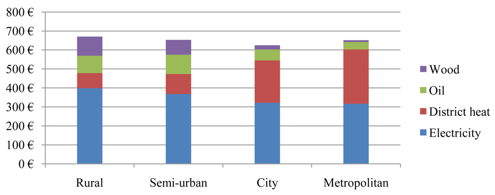
If we further analyze the components of the carbon consumption, very interestingly, the carbon emissions grow in each category but one as the degree of the urbanization grows. Energy related to housing is the largest single sector of carbon emissions. Quite surprisingly, it would seem that also the emissions related to housing energy grow as the type of region changes from detached house dominated rural regions to denser and more apartment building dominated city and metropolitan areas. The same 2.9 t CO2-eqv. carbon emissions are caused by energy use in rural and semi-urban areas with 670 € and 650 € annual expenditures, whereas in cities the figure is 3.3 t and in the Helsinki metropolitan area 3.7 t with purchases of 630 € and 650 €. While the level of energy consumption varies only slightly between the different area types, the carbon content of the energy used is slightly better in rural and semi-urban area types explaining the result. Figure 2 presents the annual energy consumption in monetary terms divided according to the utilized fuels.
Emissions from the construction and maintenance of the building (Building and property and Maintenance and operation) together form another significant entity of the total carbon consumption. In rural areas, 1.8 t CO2-eqv. emissions relate to these two categories with annual purchases of 3,000 €, whereas in the Helsinki metropolitan area the figure is as high as 2.9 t the average consumer spending 5,200 € on the commodities of these categories. In semi-urban areas the carbon consumption in these categories is 2.3 t (3,790 €) and in cities 2.6 t (4,350 €). The spending on acquisition of homes is on a substantially higher level in more urbanized areas, and the same applies to a majority of all operation and maintenance costs, explaining the differences.
The only exception in the pattern are the emissions related to private driving, which follow earlier studies i.e., [32,33] in having a growing tendency as the density of the region diminishes from the metropolitan to the rural type. In rural and semi-urban areas, the carbon consumption from private driving is 2.0 t, but in cities it is 1.6 t and in the Helsinki metropolitan area, only 1.4 t. The acquisition of vehicles equals the figures as the differences in the emissions from vehicle production are almost equal between the regions. The overall purchases on the category are 2,210 € in rural and 2,180 € in semi-urban areas, 1,910 € in cities and 1,860 € in the Helsinki metropolitan area.
Public transport slightly affects little the overall carbon consumption, but is an important low-carbon substitute for private driving. It would seem that a denser urban structure leads to higher level of public transport use, as the emissions grow from 0.05 (70 €) and 0.06 t CO2-eqv. (80 €). in rural and semi-urban areas to 0.15 (200 €) and 0.24 t (320 e) in cities and the Helsinki metropolitan area.
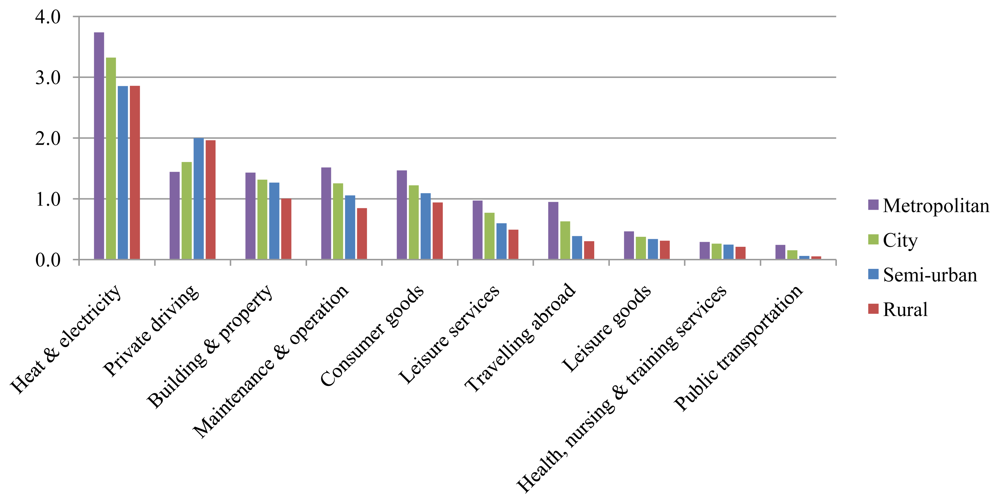
The rest of the categories comprise carbon emissions from consumption on goods and services. The share of these of the total carbon consumption varies from 25% in rural areas to 33% in the Helsinki metropolitan area, and the consumption volumes from 6,260 € to 9,270 €. The high positive connection between income and carbon consumption is also seen in these categories. In fact, these are a key explanation as to the growth in carbon consumption as the income level grows despite the region type. The pattern is very clear, as Figure 3 shows. In Figure 3, the carbon consumptions of the average consumers of the four different area types are shown sector by sector. The figure demonstrates that the emissions increase, following the growth in the volume of consumption as the income increases together with the urbanization size, in virtually every consumption sector leading thus to substantially higher overall carbon consumption in larger urbanizations.
5. Discussion
The purpose of this study was to conduct a consumption-based analysis of consumer carbon footprints for comparing the carbon emissions of average inhabitants living in different types of urban structures. This was done with four samples of consumers from Finland representing types of regions from rural to semi-urban, city and metropolitan areas. The study was conducted utilizing an application of tiered hybrid-LCA method that notifies all life cycle emissions including production and delivery chains without boundary cutoffs. We argue that this type of consumption-based modeling of emissions is of high importance and adds valuable information to more common regional production-based assessments. Especially, when seeking solutions for low-carbon living and low-carbon areal structures, consumption-based assessments of the emissions are essential.
In the study we assessed the carbon consumption of the different area types and the Finnish average consumer with the hybrid model. This assessment showed slightly unconventional results, as an average consumer of rural areas seems to cause significantly less carbon emissions than a city resident. According to the assessment, in rural areas the annual carbon consumption of an average consumer is 9.0 t CO2-eqv., in semi-urban areas 9.9 t, in cities 10.9 t and in the Helsinki metropolitan area 12.5 t.
The explanation for the unconventional result seemed to be twofold. First, it would quite unconventionally seem that the degree of urbanization, whether a rural region dominated by detached housing, or a city or metropolitan area dominated by apartment buildings, barely affects the overall emissions of an average consumer. Concerning energy consumption, which was considered to strongly favor apartment building-based city residents, the per capita monetary consumption seemed in the end to have only small variation between the different housing types. In addition, the pattern found was that the housing related emissions actually grow as the structure gets denser and housing more apartment building based due to rise in expenditure on building and maintenance following growth in the size of the urbanization. This contradicts some earlier studies, which have shown substantial differences between the carbon emissions of detached houses and apartment buildings. The explanations offered by the input data are clear, though. First, when also the communal building energy was allocated to the consumer in addition to household energy, the total amount of energy used was roughly equal in all types of regions. Second, the profile of energy sources explain the difference in emissions, as in areas with detached housing a significant amount of wood is used for heating. Also, as electricity dominates the total energy consumption in the rural areas, and has slightly better emissions profile than district heat and oil, the emissions in rural areas are lower with equal consumption volume. And third, the size of an average household is 2.33 persons in rural areas, 2.27 in semi-urban areas, 2.01 in cities and 1.93 in the Helsinki metropolitan area [22]. Even if there was difference in energy use on building level, the per capita perspective would diminish this.
The second explanation for the overall result lies in the consumption volume, 12,200 € in rural areas annually per capita, 13,800 € in semi-urban areas, 15,200 € in cities and 17,600 € in the Helsinki metropolitan area. An important pattern found in the study was that the income level and, following this, the level of consumption on goods and services grows together with the density of the structure. The consumption volume grows as the density and size of the urbanization grow in virtually all consumption sectors except private driving (see Figure 3). Now, as the volume of consumption grows, the emissions related to consumption grow. This study strongly indicates that this effect of income growth determines the volume of carbon consumption regardless of regional factors like density and housing type. Whether the more consumption-intensive lifestyle is a consequence of the growth in the size of the urbanization or not is not clear, however.
In private driving, the conventional, previously reported pattern, where emissions grow as the density decreases, was found. However, the effect on the overall carbon consumption per capita is quite weak when all the emissions related to driving are calculated, including car manufacturing, deliveries and maintenance of vehicles. According to the hybrid model, the share of fuel combustion of all private driving related emissions is 50 to 70%, the rest being dominated by car manufacturing-related emissions. Thus, growth in trip generation due to decline in the density of the city structure has only a relatively minor effect on the overall carbon consumption.
The reliability of the study was assessed from four perspectives. First, a positioning of the results among earlier applicable studies was made. Of these, calculation with the Finnish ENVIMAT study output tables showed an annual per capita carbon consumption of 10.1 t CO2-eqv. for an average Finnish consumer, whereas the figure with the hybrid model of this study was 10.3 tons. Regarding the results and the conclusions, the authors have published similar results in other recent papers [8,34]. On the method level, a reference for the applicability of the method has been published quite recently by Weber and Matthews, who used the EIO-LCA approach to study the global and distributional aspects of the American household carbon consumption [16]. Furthermore, the usefulness of the consumption-based approach has been noted in several studies. Ramaswami et al. call for the importance of exceeding the regional boundaries [35], whereas Kennedy et al. also bring up the issue stating that “it is appropriate to attribute more than just the within-boundary emissions to cities, as the consumption activities located in the cities cause the emissions” [36]. The truncation error might also be significant, i.e., [37], if boundary cutoffs are needed. Regarding this perspective the IO basis would seem very suitable for a carbon consumption assessment, as the truncation errors of all the commodities would accumulate. However, also the uncertainty (discussed further below) of the IO-based model from the utilization of industry average emissions accumulate, and create uncertainty to the results.
Second, as a test of the sensitivity of the results regarding the building-related emissions, which include some uncertainty on the allocation of the expenditure, we removed the Building and property category from the results. While the change decreases the overall emissions, the interpretation of the results remains the same. Without the sector the average annual per capita carbon consumptions of each area type are 7.3 t in rural areas, 8.0 t in semi-urban areas, 8.9 t in cities and 10.3 t in Helsinki metropolitan area.
The third source of possible biases is the hybrid model itself due to the inherent problems of all LCA approaches. Based on the assessments and amendatory actions described in the method and research design sections, we argue that we have substantially diminished these. However, especially concerning the goods and services sectors, the output sector choices include some uncertainties, as both the input data and the output sectors are quite diversified. However, the impact on the overall results is low, and no adjustments were seen to be necessary. In addition, the previously mentioned assumption of domestic production of imports is a potential source of bias. Regarding this study, this means the US industry GHG intensities for all the commodities outside of the scope of the local process data. A majority of the consumption commodities in Finland are imported, but a multi-regional model would be needed to explicitly assess the emissions. Weber and Matthews (2008) found a 15% increase in the US household carbon emissions when the imports were modeled in detail [25]. Larsen and Hertwich (2009) utilized the EIO-LCA model in Norway context, but without providing specific assessment of the potential bias of the results [24].
Finally, the reliability of the input data was assessed. In this study, the Finnish consumer survey provided the primary input data. The level of detail of the data is very high. The survey presents private consumption divided into more than 1.000 categories of goods and services, thus providing an excellent basis for IO based LCAs. Also, the sample size is representative, including roughly 10,000 subjects (0.2% of the Finnish population). In this study, the sub-samples remained sufficient (over 1,000 observations in each sample) and thus biases related to these were considered small.
Despite the very high quality input data, free public services and heavily subsidized services create a source of bias in the Finnish economy system, as these form a noteworthy share of the total private consumption. However, no amendatory actions were taken, since the assessment in the Finnish ENVIMAT study showed that the bias predominantly concerns our comprised consumption class “health, nursing and training services”, which had minor significance in this study.
As the final test of the robustness of the results, we conducted a longitudinal study using preceding consumer survey data from 2001. The test results were very similar, except for a scale difference due to the change in the income levels between the two surveys. This test strongly supports the robustness of our findings.
6. Conclusions
The study demonstrated that cities may not be more sustainable in nature compared to the surrounding suburban and rural areas concerning climate change as is often suggested, when a demand-based approach is taken. In fact, the study showed that the per capita emissions related to city lifestyle are substantially higher than those related to rural and semi-urban lifestyles in the Finnish context. This notion is very important when sustainable climate change mitigation strategies are sought in the near future. However, it is very important to notify that this study only presents a static situation of the reference year, and concluding that rural living would always be less carbon intense would be misleading. Migration from city to rural areas would probably not have any carbon mitigation effect. Thus, the main issue is to understand the huge effect of income on the overall carbon consumption, and that the type of urbanization as such does not define the emissions. It should also be noted that a very important factor behind the results of this study is the pattern of growth in the average income as the size of the urbanization grows. There might be reverse situations on a global level which could limit the generalizability of the results.
Despite the limitations, we argue that the type of consumption-based assessment approach presented here should be given high value in national- as well as regional-level decision making regarding climate change. In the future, the accuracy of the model could be further increased. In addition, comparative global studies should be conducted to test the results in different contexts.


| Rural | Semi-urban | City | Metropolitan | |
|---|---|---|---|---|
| Total population | 1,120,000 inhab. | 860,000 inhab. | 3,210,000 inhab. | 930,000 inhab. |
| Respondents in the sample | 2,200 inhab. | 1,600 inhab. | 4,700 inhab. | 1,100 inhab. |
| Level of urbanization | municipalities where <60% live in urban areas with <15,000 inhab. or 60–90% live in urban areas with <4,000 inhab. | municipalities where 60–90% live in urban areas with 4,000–15,000 inhab. | municipalities where >90% live in urban areas or with urbanizations with > 15,000 inhab. | Helsinki, Espoo and Vantaa, the capital region |
| Dominant types of housing | mainly detached | detached and small apartment buildings | mainly apartment buildings | mainly apartment buildings |
| Average household size | 2.33 | 2.27 | 2.01 | 1.93 |
| Annual volume of consumption per capita | 12,200 € | 13,800 € | 15,200 € | 17,600 € |
References
- Girardet, H. Sustainable cities: A contradiction in terms? In Environmental Strategies for Sustainable Development in Urban Areas: Lessons from Africa and Latin America; Fernandes, E., Ed.; Ashgate: Aldershot, UK, 1998. [Google Scholar]
- Satterthwaite, D. The key issues and the works included. In The Earthscan Reader in Sustainable Cities; Satterthwaite, D., Ed.; Earthscan: London, UK, 1999; pp. 3–21. [Google Scholar]
- Dodman, D. Blaming cities for climate change? An analysis of urban greenhouse gas emissions inventories. Environ. Urban. 2009, 21, 185–201. [Google Scholar]
- Carney, S.; Green, N.; Wood, R.; Read, R. Greenhouse Gas Emission Inventories for 18 European Regions; University of Manchester: Manchester, UK, 2009. [Google Scholar]
- Rauhala, K.; Mäkelä, K.; Estlander, K.; Tolsa, H.; Martamo, R.; Lahti, P.; Perälä, M. Environmentally Favorable Urban form and Transport System; Technical Research Centre of Finland: Espoo, Finland, 1997. [Google Scholar]
- Glaeser, E.L.; Kahn, M.E. The greenness of cities: Carbon dioxide emissions and urban development. J. Urban Econ. 2010, 67, 404–418. [Google Scholar]
- Norman, J.; MacLean, H.L.; Kennedy, C.A. Comparing high and low residential density: Life-cycle analysis of energy use and greenhouse gas emissions. J. Urban Plan. Dev. 2006, 132, 10–21. [Google Scholar]
- Heinonen, J.; Junnila, S. Implications of urban structure on carbon consumption in metropolitan areas. Environ. Res. Lett. 2011, 6, 014018. [Google Scholar]
- City planning will determine pace of global warming, un-habitat chief tells second committee as she links urban poverty with climate change; United Nations: New York, USA, 2007. Available online: http://www.un.org/News/Press/docs/2007/gaef3190.doc.htm (accessed on 7 April 2011).
- Suh, S.; Lenzen, M.; Treloar, G.J.; Hondo, H.; Horvath, A.; Huppes, G.; Jolliet, O.; Klann, U.; Krewitt, W.; Moriguchi, Y.; Munksgaard, J.; Norris, G. System boundary selection in life-cycle inventories using hybrid approaches. Environ. Sci. Technol. 2004, 38, 657–664. [Google Scholar]
- Junnila, S. Empirical comparison of process and economic input-output life cycle assessment in service industries. Environ. Sci. Technol. 2006, 40, 7070–7076. [Google Scholar]
- Joshi, S. Product environmental life-cycle assessment using input-output techniques. J. Ind. Ecol. 1999, 3, 95–120. [Google Scholar]
- Pandey, D.; Agrawal, M.; Pandey, J.S. Carbon footprint: Current methods of estimation. Environ. Monit. Assess. 2010, 178, 135–160. [Google Scholar]
- Matthews, H.S.; Hendrickson, C.T.; Weber, C.L. The importance of carbon footprint estimation boundaries. Environ. Sci. Technol. 2008, 42, 5839–5842. [Google Scholar]
- Carnegie Mellon University Green Design Institute. Economic input-output life cycle assessment (EIO-LCA), US 2002 industry benchmark model [Internet]. Carnegie Mellon University Green Design Institute: Pittsburgh, USA, 2008. Available online: http://www.eiolca.net/ (accessed on 1 February 2010). [Google Scholar]
- Weber, C.L.; Matthews, H.S. Quantifying the global and distributional aspects of American household carbon footprint. Ecol. Econ. 2008, 66, 379–391. [Google Scholar]
- Sharrard, A.L.; Matthews, H.S.; Ries, R.J. Estimating construction project environmental effects using an input-output-based hybrid life-cycle assessment model. J. Infrastruct. Syst. 2008, 14, 327–336. [Google Scholar]
- Crawford, R. Life Cycle Assessment in the Built Environment; Spon Press: London, UK, 2011. [Google Scholar]
- Statistics Finland. The Finnish Consumer Survey 2006, the Data not Publicly Available; Statistics Finland: Helsinki, Finland, 2007. [Google Scholar]
- Seppälä, J.; Mäenpää, I.; Mattila, T.; Nissinen, A.; Katajajuuri, J-M.; Härmä, T.; Korhonen, M-R.; Saarinen, M.; Virtanen, Y.; Koskela, S. Assessment of the environmental impacts of material flows caused by the Finnish economy with the ENVIMAT model (Suomen kansantalouden materiaalivirtojen ympäristövaikutusten arviointi ENVIMAT-mallilla); Finnish Environment Institute (SYKE): Helsinki, Finland, 2009. [Google Scholar]
- Lenzen, M.; Pade, L.-L.; Munksgaard, J. CO2 multipliers in multi-region input-output models. Econ. Syst. Res. 2004, 16, 391–412. [Google Scholar]
- Statistics Finland. Statistics Finland: Helsinki, Finland, 2009. Available online: http://www.stat.fi/ (accessed on 15 December 2009).
- World Resources Institute. Greenhouse Gas ProtocolInitiative: New Guidelines for Product and Supply ChainAccounting and Reporting; World Business Council for Sustainable Development: Geneva, Switzerland, 2009. [Google Scholar]
- Larsen, H.N.; Hertwich, E.G. The case for consumption-based accounting of greenhouse gas emissions to promote local climate action. Environ. Sci. Policy 2009, 12, 791–798. [Google Scholar]
- Weber, C.L.; Matthews, H.S. Quantifying the global and distributional aspects of American household carbon footprint. Ecol. Econ. 2008, 66, 379–391. [Google Scholar]
- International Bank for Reconstruction and Development, The World Bank. Global Purchasing Power Parities and Real Expenditures; International Bank for Reconstruction and Development, The World Bank: Washington, DC, USA, 2008. [Google Scholar]
- Kurnitski, J.; Keto, M. Emissions from Building Energy Consumption and Primary Energy Use in Finland (Rakennusten energiankäytön aiheuttamat päästöt ja primäärienergiankäyttö). unpublished work.
- Kyrö, R.; Heinonen, J.; Säynäjoki, R.; Junnila, S. Climate Impact of Housing Companies—A Hybrid LCA Approach. Proceedings of 2011 2nd International Conference on Environmental Science and Technology (ICEST 2011), Singapore, 26–28 February 2011.
- Kiiras, J.; Saari, A.; Hyart, J.; Kammonen, J. Property Maintenance Expenses in Finland 1992 (Kiinteistöjen ylläpidon kustannustieto 1992); Helsinki University of Technology: Espoo, Finland, 1993. [Google Scholar]
- VTT Technical Research Centre of Finland. “LIPASTO—Unit emissions—Passenger traffic—Road traffic,” 2010. VTT Technical Research Centre of Finland: Espoo, Finland, 2010. Available online: http://lipasto.vtt.fi/yksikkopaastot/henkiloliikennee/tieliikennee/henkilo_tiee.htm (accessed on 1 March 2010). [Google Scholar]
- The Housing Finance and Development Centre of Finland (ARA). Reports A 12/2006; The Housing Finance and Development Centre of Finland (ARA): Lahti, Finland, 2006. [Google Scholar]
- WSP Finland Ltd. Passenger Transport Survey 2004–2005. WSP Finland Ltd.: Helsinki, Finland, 2005. Available online: http://www.hlt.fi/english/index.htm (accessed on 7 April 2011). [Google Scholar]
- Kivari, M.; Voltti, V.; Heltimo, J.; Moilanen, P. Impact of the Type and Location of the Residentialarea on Travel Behaviour; Finnish Road Administration: Helsinki, Finland, 2007. [Google Scholar]
- Heinonen, J.; Junnila, S. Metropolitan Carbon Management, A Hybrid-LCA Approach. Proceedings of 2011 2nd International Conference on Environmental Science and Technology (ICEST 2011), Singapore, 26–28 February 2011.
- Ramaswami, A.; Hillman, T.; Janson, B.; Reiner, M.; Thomas, G. A demand-centered, hybrid life-cycle methodology for city-scale greenhouse gas inventories. Environ. Sci. Technol. 2008, 42, 6455–6461. [Google Scholar]
- Kennedy, C.; Steinberger, J.; Gasson, B.; Hansen, Y.; Hillman, T.; Havránek, M.; Pataki, D.; Phdungsilp, A.; Ramaswami, A.; Villalba Mendez, G. Greenhouse gas emissions from global cities. Environ. Sci. Technol. 2009, 43, 7297–7302. [Google Scholar]
- Huang, Y.A.; Lenzen, M.; Weber, C.L.; Murray, J.; Matthews, H.S. The role of input-output analysis for the screening of corporate carbon footprints. Econ. Syst. Res. 2009, 21, 217–242. [Google Scholar]
- Conflict of Interest: The authors declare no conflict of interest.
© 2011 by the authors; licensee MDPI, Basel, Switzerland. This article is an open access article distributed under the terms and conditions of the Creative Commons Attribution license (http://creativecommons.org/licenses/by/3.0/).
Share and Cite
Heinonen, J.; Junnila, S. A Carbon Consumption Comparison of Rural and Urban Lifestyles. Sustainability 2011, 3, 1234-1249. https://doi.org/10.3390/su3081234
Heinonen J, Junnila S. A Carbon Consumption Comparison of Rural and Urban Lifestyles. Sustainability. 2011; 3(8):1234-1249. https://doi.org/10.3390/su3081234
Chicago/Turabian StyleHeinonen, Jukka, and Seppo Junnila. 2011. "A Carbon Consumption Comparison of Rural and Urban Lifestyles" Sustainability 3, no. 8: 1234-1249. https://doi.org/10.3390/su3081234