
Sustainable Suppliers-to-Consumers’ Sales Mode Selection for Perishable Goods Considering the Blockchain-Based Tracking System


Faculty of Management and Economics, Kunming University of Science and Technology, Kunming 650504, China
*
Author to whom correspondence should be addressed.
Sustainability 2024, 16(8), 3433; https://doi.org/10.3390/su16083433
Submission received: 25 February 2024
/
Revised: 14 April 2024
/
Accepted: 16 April 2024
/
Published: 19 April 2024
Abstract
:Given the significant product spoilages of perishable goods transported over long distances, they are usually sold from suppliers to consumers through an offline direct channel. Sustainable suppliers can utilize the blockchain-based tracking system (BTS) to reduce product spoilages, enabling the spoilage reduction effect, and offer authentic information, triggering the premium effect. With the advent of e-commerce, they can now opt for an online direct channel, setting the online direct price as either non-different or different from the offline direct price, and have to face challenges in selecting the optimal sales mode. This paper addresses these complexities by developing a mathematical model to construct a sustainable suppliers-to-consumers pricing model, incorporating the BTS, in the perishable goods market. Our research reveals that the decision to adopt the BTS hinges on factors like the spoilage reduction effect, premium effect, production cost, and tag cost, with the premium effect outweighing the spoilage-reduction effect. The necessity of using the BTS grows with extended circulation times, where the BTS significantly reduces spoilages during transportation, fostering sustainable development. While sustainable suppliers may not always bear the tag cost independently, they can adjust their pricing strategies automatically and pass the tag cost to consumers for more profit. The BTS adoption decision does not influence the optimal sales mode selection strategy. The offline direct channel offers the highest profit for suppliers, followed by the Online to Offline (O2O) direct channel with differential pricing, and the O2O direct channel with non-differential pricing yields the lowest profit.
1. Introduction
The perishability, short shelf life, and susceptibility to damage of perishable goods during long-distance transportation often result in serious product spoilages, encompassing both quality and quantity spoilages [1]. These spoilages lead to substantial economic losses for enterprises [2,3], and raise environmental concerns. The label fraud incident involving Freshippo in China has drawn consumers’ attention to the authentic information of perishable goods [4]. The implementation of a blockchain-based tracking system (BTS) presents a solution to these challenges [5]. By utilizing the open, transparent, and immutable characteristics of blockchain technology, the BTS helps to reduce product spoilages of perishable goods to achieve sustainable development, enabling about a spoilage reduction effect, and provide authentic information, triggering the premium effect [4]. Many enterprises, like Decanter in the Netherlands, Aglive in Australia, and FinComEco in Africa, recognize the importance of adopting the BTS to reduce product spoilages and ensure authenticity [6]. Despite these benefits, the significant costs associated with the implementation of the BTS affect the decision-making process for its implementation. Some companies, like Sunkist and Dairy Farmers of America, may hesitate to embrace the BTS due to these costs [4]. As living standards rise, consumers increasingly prioritize the freshness of perishable goods and authentic information. Therefore, we introduce the BTS to enable a spoilage reduction effect and a premium effect for sustainable suppliers.
Due to the perishability of perishable goods, it is crucial for sustainable suppliers to select an appropriate sales mode. The rapid advancement of Internet technology and the remarkable success of e-commerce have significantly altered consumer shopping behaviors, prompting many sustainable suppliers to constantly revamp their sales models to boost their profits [7]. In China, there are currently a large number of suppliers for whom the sale of perishable goods is a vital income source [8]. Consequently, it is imperative to address the following issues arising from this trend. Firstly, some sustainable suppliers, like Decanter in the Netherlands and Aglive in Australia, directly distribute perishable goods to consumers through an offline direct channel, such as their physical stores. Secondly, sustainable suppliers such as Tuotuo Gongshe sell perishable goods to consumers through online direct channels, like their official websites, WeChat mini-programs, and WeChat public accounts. However, the online direct channel cannot provide consumers with a perfect consumption experience, and many suppliers, such as MISSFRESH, have gone bankrupt [9]. The sales volume of the online direct channel is relatively low, and we therefore do not study this channel; Thirdly, sustainable suppliers, such as Baiguoyuan, sell perishable goods to terminal consumers through offline direct physical stores and online direct channels, wherein the online direct price is not different from the offline direct price. Finally, sustainable suppliers, like Yipin Shengxian and Huajia, not only sell perishable goods to terminal consumers through offline direct physical stores but also through online direct channels, wherein the online direct price is different from the offline direct price. Based on these business practices, we investigate three typical sales modes, the offline direct channel, the O2O direct channel with non-differential pricing, and the O2O direct channel with differential pricing, to explore the optimal sales mode from the perspectives of sustainable suppliers with the BTS.
This paper aims to address the following issues: (i) How does BTS adoption affect the equilibrium profit of the suppliers across three different suppliers-to-consumers’ sales modes, such as the offline direct channel, the O2O direct channel with non-differential pricing, and the O2O direct channel with differential pricing? (ii) What is the optimal sales mode for the suppliers in both the absence and presence of the BTS? (iii) How does BTS adoption affect the sales mode selection? To address the suppliers’ selection of their sales mode, we first consider the BTS’s enabling of the spoilage reduction effect and the premium effect in the direct perishable goods market. Firstly, we use a mathematical model to construct the offline direct pricing model for the offline direct channel, before and after adopting the BTS. Secondly, we employ the mathematical model to build the offline and online direct pricing models for the O2O direct channel with non-differential pricing, before and after adopting the BTS. Thirdly, we use the mathematical model to construct the offline and online direct pricing models for the O2O direct channel with differential pricing, before and after adopting the BTS. Finally, by comparing and analyzing the optimal strategies under three different suppliers-to-consumers’ sales modes, we obtain the optimal sales mode selection strategy for suppliers theoretically and numerically.
The key findings of our study can be summarized as follows. Firstly, sustainable suppliers are motivated to shorten the circulation time and lower the production cost of their goods. Secondly, sustainable suppliers are more inclined to adopt the BTS than the intelligent logistics system (ILS), which may not always bear the tag cost alone. They adjust their pricing strategies automatically and pass on the tag cost to consumers for more profit. Thirdly, the application of the BTS may not always be advantageous for suppliers. Factors such as the spoilage reduction effect, premium effect, production cost, and tag cost influence the decision to use the BTS under different channels, like offline direct and O2O direct with non-differential pricing. Moreover, under the O2O direct channel with differential pricing, the market size of the offline direct channel, cross-price elasticity, and other factors play a role in the decision-making process. The premium effect is deemed more crucial than the spoilage reduction effect in determining the BTS adoption. Additionally, the necessity of using the BTS increases with longer circulation times, where the BTS significantly reduces spoilages during transportation, contributing to sustainable development. Finally, regardless of the BTS adoption, the offline direct channel remains the optimal sales mode for suppliers. The BTS adoption decision does not affect the optimal sales mode selection. In the process of adopting the BTS, maintaining the original sales model may be the non-optimal practical sales mode selection strategy for sustainable suppliers.
The rest of the paper is organized as follows: Section 2 reviews the relevant literature; Section 3 presents the models; Section 4 lays out the analytic results, compares the models’ analytic results, and presents some managerial implications; and Section 5 summarizes the results and gives future research directions. All proofs are included in Appendix A.
2. Literature Review
We categorize the literature related to our study into two streams: the application of the blockchain-based tracking system in the perishable goods supply chain and the selection of sales modes discussed in the following section.
The first related research area focuses on the application of the blockchain-based tracking system in the perishable goods market from various perspectives, such as the spoilage reduction effect [1,3,5,10,11,12,13], premium effect [4,14,15,16,17], tag cost [18,19,20], supply chain coordination [5,10,21], and adoption strategy [22,23,24]. The characteristics of perishable goods, such as their perishability and susceptibility to deterioration, make the supplier and retailer highly susceptible to product spoilages during production, transportation, and retailing [1,3,5], which poses environmental concerns. Cai et al. [10] examined the optimal way to maintain freshness throughout transportation. As one of the critical technologies of the intelligent logistics system (ILS) [11], Radio Frequency Identification (RFID) technology can partially or entirely eliminate the risk of logistics-related spoilages [12]. These efforts have led to a notable decrease in carbon emissions by cutting fuel consumption and resource utilization, promoting sustainable development. While the ILS collects data throughout the entire process, alleviating consumer concerns to some extent, the ability of supply chain members to freely alter information has heightened consumer apprehension and failed to generate a premium effect for consumers [5,13]. In addition to the spoilage reduction effect enabled by the ILS, the BTS can also provide authentic information and trigger the premium effect [4]. The systems with traceability capabilities, such as the blockchain-based tracking system (BTS), provide various benefits, including reducing product spoilages, offering authentic information, traceability, and immutability, which are the most critical factors in implementing the BTS [17]. Urban consumers in China are most willing to pay for government-certified traceable milk [15]. Consumers are willing to pay a 25% premium for organic apples that provide related information and a 42% premium for information on origin, ingredients, and other details [14]. Galati et al. [16] indicated that consumers are willing to pay a premium for natural wine, depending on the content, production process, and taste attributes listed on the wine label. Liu et al. [18] investigated the impact of the fixed cost and the operational cost of the BTS on a supply chain dominated by the imported perishable goods supplier, retailer, and a blockchain platform. Jensen et al. [19] identified the investment cost associated with the BTS as a significant barrier to its widespread application. However, with the rapid expansion and application of Internet of Things (IoT) systems, related costs have decreased and are expected to continue declining [20]. By integrating the preservation effort, Cai et al. [10] developed a supply chain coordination model to eliminate product spoilages, including quantity spoilage and quality degradation during the flow process. Wu et al. [5] found that, in a fresh product supply chain composed of the supplier, third-party logistics provider, and e-commerce retailer, the leader should provide a two-part tariff contract to support the smooth implementation of the BTS. However, not all supply chain contracts can achieve coordination in food supply chains that incorporate blockchain technology and comprise suppliers and retail platforms. The cost-sharing contract cannot achieve supply chain coordination, while the revenue-sharing contract, profit-sharing contract, and two-part tariff contract can [21]. Aiello et al. [22] analyzed the traceability system’s expected value and optimal granularity level for perishable goods, such as fruits and vegetables. Saak [23] pointed out that perfect traceability is not always the optimal solution for the supply chain involving a single retailer and multiple suppliers. Niu et al. [24] employed a Stackelberg game model to analyze the blockchain technology investment decisions in the perishable goods supply chain, which is composed of two competing suppliers and a dominant retailer.
Existing research indicates that the BTS can effectively reduce product spoilages, achieve sustainable development, provide authentic information, and enhance consumer purchase intention. However, the functionality of the BTS is rarely analyzed from the perspectives of the spoilage reduction and premium effects. Building on this existing literature, we examine the impact of the BTS, which reduces product spoilages and offers authentic information in the perishable goods market.
The second related research area concerns the suppliers’ selection of sales mode. The suppliers’ sales modes are where the supplier sells products directly to consumers through offline direct and online direct channels and undertakes the production, logistics, and retail functions [7,25]. Depending on the suppliers’ sales mode selection, they choose between the offline direct channel [24,25,26,27], online direct channel [9,28,29], O2O direct channel with non-differential pricing [30,31], and O2O direct channel with differential pricing [32,33]. In China, perishable goods are mainly sold through the supplier’s offline direct channel, which operates in a coordinated state [25]. The farmer direct sales model is the most efficient sales model for circulation [26]. Li et al. [27] investigate the optimal advertising decisions of new and remanufactured products under the offline direct channel. Chen et al. [28] conducted a case study on Tianbao bananas produced and sold in Zhangzhou, constructing an efficiency system based on the circulation cost, circulation expense rate, profit margin, and producer–share ratio. The supplier can sell products to consumers directly through a platform that imposes a commission fee, such as JD.COM [29]. The online direct channel cannot provide consumers with a perfect consumption experience, and the sales volume of online channels is relatively low [9]. Thus, the online suppliers’ sales channel is not within the scope of our research. Given that the O2O channel with non-differential pricing and the O2O channel with differential pricing both fall under the O2O channel, this study categorizes them together for evaluation. The main manifestations of the combined offline and online direct channels include the community’s weekend vegetable offline suppliers-to-consumers’ sales market, community sales service stations, and online distribution channels. Beijing Lvfulong Cooperative opened community weekend offline direct markets in the Beihang and Wangjing communities and launched online intelligent sales models in areas like the Meteorological Bureau residential area [30]. For enterprises with both online and offline channels, their dual-channel sales prices are identical approximately 72% of the time [31]. The difference in sales prices between the two channels depends on the type of enterprise and consumers’ shopping risk [32]. In real life, many large-scale perishable goods suppliers are located in the suburbs of cities, where they sell pollution-free, green, and organic vegetables through offline physical stores and online direct channels in urban areas. In addition to the offline direct channel, sustainable suppliers can use the commission rate to sell green products to consumers directly through e-commerce platforms [33].
The above studies highlight the significance of the suppliers-to-consumers’ sales mode for perishable goods, emphasizing sales mode innovation led by the supplier. However, the research on the suppliers’ selection of sales mode among the online direct channel, the O2O channel with non-differential pricing, and the O2O channel with differential pricing is insufficient. In this context, we consider the BTS, which enables spoilage reduction and premium effects, and examine how suppliers select their sales mode within these three options.
3. Problem Description and Assumptions
We consider sustainable suppliers, which sell perishable goods directly to terminal consumers. These suppliers and consumers are typically located in the same city or region, with suppliers residing in suburban areas. The supplier can distribute perishable goods to consumers through offline and online direct channels. In the offline direct channel, consumers purchase perishable goods from the supplier’s direct physical stores, while in the online direct channel, consumers buy perishable goods from the supplier’s WeChat public accounts, mini programs, WeChat groups, moment, or QQ groups. Then, the supplier delivers the perishable goods to the consumers. Thus, the supplier has the following three common suppliers-to-consumers’ sales modes (see Figure 1): (i) the offline direct channel, where the supplier can exclusively sell perishable goods to consumers through its direct physical stores; (ii) the O2O direct channel with non-differential pricing, where the supplier directly sells perishable goods to consumers through both offline and online direct channels at the same direct prices; and (iii) the O2O direct channel with non-differential pricing, where the supplier directly sells perishable goods to consumers through both offline and online direct channels at the different direct prices.
When the supplier implements the BTS, consumers in the offline direct channel can obtain complete and authentic product information by scanning the QR code on the product or packaging. Consumers in the online direct channel can access comprehensive and authentic information the supplier provides about the production, logistics, and retail processes. They can then verify this authentic information upon receiving the perishable goods. The availability of detailed authentic information enables consumers to assess the freshness better, boost their confidence in making purchases, and even be willing to pay a premium for it [6]. As previously mentioned, the ILS cannot address the issue of intentional tampering with information; therefore, the BTS can meet consumers’ demands for authentic information, triggering a premium effect of authentic information.
Firstly, the BTS enables spoilage reduction and premium effects. The spoilage reduction effect means that product spoilage is reduced and freshness is improved to achieve sustainable development. Specifically, the survival rate and freshness of products arriving in the market have increased. On the one hand, the survival rate, , , decreases with the elapse of the circulation time [5], where is the deterioration rate of physical quantity. If the circulation time is closer to the product lifecycle, the product survival rate tends to be zero. Therefore, we have and . Assuming that units of perishable goods are transported from the initial supplier to the end consumer market, the final product survival quantity is units. On the other hand, the freshness decreases with the passage of circulation time, where is the decay rate of freshness [34,35]. Based on the actual situation, we assume that , , and . According to practical experience, freshness is closely related to product survival rate. Following the literature (e.g., [4]), to avoid unnecessary conclusions, freshness and product survival rate are equal, . The United States has well-equipped cold supply chain equipment and systems, and the spoilage of perishable goods accounts for 1–5% of total product output. Meanwhile, following the research (e.g., [12]), the BTS can completely eliminate the risk of logistics-related spoilages; after the BTS is adopted, the product freshness and survival rate are both 1, . Simultaneously, we set to describe low-quality perishable goods and to describe high-quality perishable goods. We define the spoilage reduction effect function, , which has the characteristic of decreasing with increasing freshness and . The spoilage reduction effect is a strictly monotonically decreasing function of freshness and a strictly monotonically increasing function of circulation time. For the convenience of analysis, we use freshness to characterize the characteristics of the spoilage reduction effect. The longer the circulation time, the greater the product spoilages generated. Once the BTS is adopted, the more it can promote the achievement of sustainable development. On the other hand, the premium effect means consumers are willing to pay a certain degree of premium for products that provide authentic and complete information. Under the BTS, authentic and complete information can enhance consumer confidence, attract more consumers, and even make consumers willing to pay a certain premium to purchase perishable goods with complete information [6,14,36]. Consumers purchase perishable goods from the online direct channel at the direct price set by the supplier, and the premium value for consumers is . Similarly, the premium value for consumers in online direct channels is . The 2020 China Fresh Supply Chain Industry Research Report released by iResearch shows that nearly 82% of Chinese consumers are willing to pay a premium of no more than 20% for products with quality certification information. Given this, we assume that each consumer is willing to pay a premium to purchase perishable goods with the BTS, , , and represents the premium effect.
Secondly, when suppliers opt for the offline direct channel without the BTS, the channel demand is negatively correlated with the direct price and positively correlated with freshness. Once consumers enter the market, their purchasing decisions are influenced by the product’s direct price and freshness. Therefore, according to prior studies [3,37,38,39], the demand function for the offline direct channel is expressed as follows:
where represents the total market size in the offline direct channel without the BTS, measures the impact of the offline direct price on the demand for the offline direct channels, and represents the freshness without the BTS.
Thirdly, when sustainable suppliers apply the BTS, the demand function for perishable goods is closely related to the direct price and freshness and is positively correlated with the premium effect. In other words, once consumers enter the market, each consumer is willing to pay a premium for the complete and valuable authentic information provided by the supplier and retailer. With reference to the literature (e.g., [3,37,38,39]), the demand function for the offline direct channel is as follows:
where represents the total market size in the offline direct channel with the BTS, represents the freshness with the BTS, measures the impact of the offline premium on the demand for the offline direct channel, and represents the premium value of the offline direct channel. Following the literature (e.g., [38,39]), we set , , and .
Fourthly, in the absence of the BTS, when suppliers choose the O2O direct channel with non-differential pricing, the offline direct price is equal to the online direct price, . Referring to the research of Ji et al. [13], Huang and Swaminathan [40], and Tang and Yang [41], the demand functions for offline and online direct channels are expressed as follows:
When suppliers choose the O2O direct channel with differential pricing, the demand function follows a linear model of channel substitutability: (i) the demand for each channel is negatively correlated with its own channel price and positively correlated with freshness; and (ii) the demand for each channel is positively correlated with the prices of competing channels. With reference to the literature (e.g., [3,4,7,37,38,39,42,43,44,45]), the demand functions for offline and online direct channels are as follows:
where represents the total market size in the O2O direct channel with non-differential pricing without the BTS, represents the total market size in the O2O direct channel with differential pricing without the BTS, measures the impact of the direct price on the demand for the direct channel, and explains the degree of competition between the offline and online direct channels in terms of the price behavior. The price elasticity coefficient is greater than the cross-price elasticity coefficient, which means that the influence of the direct price on their own channel is greater than that on a competitive channel, .
Fifthly, in the presence of the BTS, consumers in both offline and online direct channels are willing to pay a premium for perishable goods with authentic information. This means that consumers purchasing perishable goods from the offline direct channel at the direct price have a premium value of . Similarly, consumers in the online direct channel have a premium value of . When sustainable suppliers choose the O2O direct channel with non-differential pricing, the direct prices and premium values in both offline and online direct channels are equal: and . Referring to the research of Cattani et al. [46], Zhou et al. [47], and Rahmani and Yavari [48], the demand functions for offline and online direct channels are expressed as follows:
When sustainable suppliers choose the O2O direct channel with differential pricing, the demand function follows a linear model of channel substitutability: the demand for each channel is negatively correlated with its own channel price, positively correlated with freshness and its own channel premium; and the demand for each channel is positively correlated with the prices of the competing channel and negatively correlated with the premium of the competing channel. Following the literature (e.g., [3,4,7,37,38,39,42,43,44,45]), the demand functions for offline and online direct channels are expressed as follows:
where represents the total market size in the O2O direct channel with non-differential pricing with the BTS, represents the total market size in the O2O direct channel with differential pricing with the BTS, measures the impact of the premium effect on the demand for the direct channel, and explains the degree of competition between the offline and online direct channels in terms of the premium behavior. The price elasticity coefficient is greater than the cross-price elasticity coefficient, which means that the influence of the premium effect on its own channel is greater than that on its competitive channel, . Following the literature (e.g., [4,38,39,44]), we set the following parameters: , , , , , and .
Sixthly, the implementation of the BTS involves essential components like the fundamental information technology structure, fixed readers, and smart tags, incurring significant investment costs. Following the literature (e.g., [5,11,35,49]), the tag cost, encompassing the cost of providing authentic information, such as seeds, perishable good attributes, pesticides, country of origin, logistics, and retailing information, poses a significant obstacle to the BTS implementation decisions. According to the literature (e.g., [35]), represents the production cost per unit of perishable goods, including seeds, pesticides, labor, logistics, and other input costs.
Finally, to analyze the BTS’s impact on supplier decisions effectively, the following assumptions are made. Firstly, an insufficient supply of perishable goods results in inadequacy, with no surplus supplied to the offline or online direct channels. Both direct channels have loyal consumers, and . In the offline direct channel, perishable goods are harvested, processed, and transported to the supplier’s offline direct channel, where terminal consumers purchase them. In the online direct channel, perishable goods are harvested, processed, and transported directly to terminal consumers. All consumers in the offline and online direct channels and suppliers are in the same cities or regions. Therefore, the circulation time for perishable goods in offline and online direct channels is roughly equivalent. Furthermore, assuming that consumer inflow and outflow in a specific region or city are balanced, we consider the potential market size of consumers in the region to be constant, indicating a fixed total consumer market size. For simplicity, without loss of generality and for analytical convenience, following the literature (e.g., [4,9]), we assume that . Secondly, following the literature (e.g., [4,5]), the ILS can automatically identify perishable goods, quickly read data, shorten the time during the flow process, and reduce product spoilages using real-time monitoring and controlling the temperature and humidity during the flow process. Based on this, blockchain technology is used to provide authentic product information. Therefore, compared to the ILS, the marginal cost of generating traceability system labels containing blockchain technology is zero, after applying the BTS. Thirdly, to ensure the model’s effectiveness and avoid invalid results, we assume that and . Table 1 summarizes all the symbols involved in this section.
4. Equilibrium Analysis
These discussions are based on the limitations in the supplier’s selections of sales modes. On the one hand, we explore the pricing strategies without and with the BTS under three distinct sales modes: the offline direct channel, the O2O direct channel with differential pricing, and the O2O direct channel with differential pricing. On the other hand, we conduct a comparative analysis of the equilibrium strategies among these sales modes to ascertain the optimal sales mode selection for the supplier.
4.1. Offline Direct Channel
When the supplier opts for the offline direct channel, an optimal offline direct pricing model is developed for Scenarios I and II, based on whether the supplier adopts the BTS. We compare and analyze the condition under which the supplier adopts the BTS in the offline direct channel.
4.1.1. Scenario I: Without the Blockchain-Based Tracking System
When opting not to adopt the BTS, the supplier aims to maximize its profit by setting the optimal offline direct price. Therefore, the expected profit for the supplier is as follows:
Lemma 1.
When , the equilibrium offline direct price is , the equilibrium offline direct quantity is , and the equilibrium profit of the supplier is .
Lemma 1 reveals two key points. On one hand, the supplier’s equilibrium profit is negatively correlated with the production cost. As the production cost increases, the offline direct price rises, leading to lower consumer purchase volume and reducing the supplier’s equilibrium profit. This aligns with the realities of agricultural production. On the other hand, the supplier’s equilibrium profit decreases as the circulation time increases. The longer the circulation time, the longer the distance traveled, and the more the product spoilages. This results in a higher consumer purchase price, weaker purchase intentions, and ultimately lower purchase volume, reducing equilibrium profit for the supplier. Thus, the supplier is incentivized to take measures, such as implementing the BTS, to lower the production cost, shorten circulation time, and ultimately reduce product spoilages.
4.1.2. Scenario II: With the Blockchain-Based Tracking System
The suppliers leverage the BTS to simplify operational processes, shorten circulation time, and reduce product spoilages through automatic product identification and data collection. Simultaneously, consumers are willing to pay an additional premium for the perishable goods with the BTS. After implementing the BTS, sustainable suppliers readjust the online direct price to maximize their profit. Therefore, the expected profit for the supplier is expressed as follows:
Lemma 2.
When , the equilibrium offline direct price is , the equilibrium offline direct quantity is , and the equilibrium profit of the supplier is .
Through Lemma 2, it can be seen that the equilibrium profit of suppliers is positively correlated with the premium effect, and negatively correlated with the production and tag costs, which is also consistent with the production practice of perishable goods. The higher the premium effect, the stronger the consumers’ willingness to purchase, the larger the purchase quantity, and thus the greater the supplier’s equilibrium profit. For the supplier, adopting the BTS means an increase in costs, with a significant proportion of its revenue used to offset the negative impact of the tag cost.
4.1.3. Comparative Analysis of Equilibrium Strategies with and without the Blockchain-Based Tracking System
Firstly, the equilibrium outcomes of the supplier without and with BTS are compared, and the decision conditions for the supplier to apply the BTS are obtained.
Proposition 1.
(i) When the tag cost is low (), the supplier reduces the offline direct price. When the tag cost is high (), the supplier improves the offline direct price, where .
(ii) When the tag cost is low (), the supplier obtains the higher offline direct quantity. When the tag cost is high (), the supplier obtains the lower offline direct quantity, where .
(iii) When the tag cost is low (), the supplier obtains a higher equilibrium profit. When the tag cost is high (), the supplier obtains a lower equilibrium profit, where .
Proposition 1 highlights that the supplier does not always shoulder the tag cost alone in the offline direct channel. Instead, it automatically adjusts its offline pricing strategies and passes on the tag cost to consumers to achieve more profit. Additionally, implementing the BTS does not always result in higher offline direct quantity. Finally, it is not always profitable for the supplier to adopt the BTS strategy (see Figure 2).
Proposition 2.
(i) When the freshness is low (), the supplier reduces the offline direct price. When the freshness is high (), the supplier improves the offline direct price, where .
(ii) When the freshness is low (), the supplier obtains the higher offline direct quantity. When the freshness is high (), the supplier obtains the lower offline direct quantity, where .
(iii) When the freshness is low (), the supplier obtains a higher equilibrium profit. When the freshness is high (), the supplier obtains a lower equilibrium profit, where .
Proposition 2 shows that the supplier in the offline channel is unable to implement the BTS for all perishable goods. Only perishable goods with sufficiently low freshness are suitable (see Figure 2). That is to say, the longer the circulation time, the stronger the necessity of using the BTS for perishable goods. In this case, the spoilage reduction effect enabled the BTS is significant, highlighting that the more spoilages generated by the transportation of perishable goods are reduced, the more conducive it is to achieve sustainable development.
Proposition 3.
Comparing the equilibrium profits of suppliers without and with the BTS, we can examine the significant impact of the spoilage reduction effect and the premium effect on the supplier’s decision to adopt the BTS.
(i) When the premium effect is at a high level (), the application of the BTS is profitable for the supplier ().
(ii) When both the premium effect and the tag cost are at a low level ( and ), the application of the BTS is profitable for the supplier (). Otherwise, it is detrimental for the supplier (), where and .
Proposition 3 guides the optimal sales strategy for the supplier in the offline direct channel, outlining how the decision to implement the BTS is influenced by changes in the spoilage reduction effect (i.e., freshness spoilage reduced and quantity spoilage reduced), premium effect, production cost, and tag cost. It suggests that the supplier is always motivated to invest in the BTS when the premium effect outweighs the spoilage reduction effect. The positive impact solely resulting from a strong premium effect can offset the negative impact of the tag cost. In conclusion, the premium effect is a crucial indicator for the supplier in adopting the BTS and adjusting its online pricing strategies.
Furthermore, the spoilage reduction effect may not always motivate the supplier to adopt the BTS. Particularly when the premium effect becomes milder relative to the spoilage reduction effect, and both the premium effect and the tag cost are low, it is advisable for the supplier to implement the BTS.
Moreover, it is evident that in the process of adopting the BTS, the premium effect holds more significance than the spoilage reduction effect. It is also apparent that adopting the BTS is not always an optimal strategy for the supplier, especially under the offline direct channel, which directly explains the diverse attitudes of companies towards BTS adoption. Deloitte’s Global Blockchain Survey indicates that in 2020, only 70.9% of multinational companies, despite recognizing the importance of blockchain technology, actually integrated it into their production processes. Therefore, the supplier’s focus on adopting the BTS should be on providing authentic, comprehensive, and valuable information to generate a higher premium effect, thus mitigating the challenges associated with the BTS adoption.
Next, by taking the non-existent premium effect () as the baseline, i.e., adopting the ILS, we thoroughly analyze the impact of the premium effect on the supplier’s equilibrium profit. By incorporating it into Proposition 3, we can derive Corollary 1.
Corollary 1.
For a given tag cost and non-existent premium effect (), comparing the equilibrium profit of the supplier between without and with the BTS, when the tag cost is at a low level (), adopting the BTS or ILS is more profitable to the supplier (); otherwise, it is detrimental for the supplier ().
By combining Proposition 3 and Corollary 1, it becomes evident that the ILS is more likely to be accepted than the BTS. The premium effect makes the supplier of the offline direct channel more likely to adopt the BTS. Specifically, in the absence of a premium effect, as seen in the ILS, the positive impact of the spoilage reduction effect cannot always fully counteract the negative impact of the tag cost. However, in a scenario with a high-level premium effect, the supplier is still motivated to invest in the BTS, even without the spoilage reduction effect. In the presence of the premium effect, the comprehensive positive effects, including the spoilage reduction effect and the premium effect, are more likely to offset the negative impact of the tag cost completely. Furthermore, in cases where the positive impact generated by a sufficiently high premium effect completely offsets the negative impact of the tag cost, the premium effect assumes a more critical role than the spoilage reduction effect in the supplier’s decision-making process regarding adopting the BTS.
Finally, we examine the impact of the freshness, production cost, premium effect, and tag cost on the equilibrium profit of the supplier.
Corollary 2.
Given the freshness, production cost, premium effect, and tag cost, we aim to investigate their impact on the equilibrium profit of the supplier without and with the BTS.
(i) In equilibrium (), the equilibrium profit of the supplier is positively correlated with the freshness () and negatively correlated with the production cost ().
(ii) In equilibrium (), the equilibrium profit of the supplier is positively correlated with the premium effect () and negatively correlated with the production cost and tag cost ( and ).
(iii) Compared to the scenario with no premium effect (), the premium effect always benefits the supplier.
In Figure 2, taking and as an example, it is evident that the impact of the premium effect on the equilibrium profit of the supplier is monotonic. Additionally, there are inflection points in the equilibrium profit of the supplier, as shown in Figure 2. These inflection points occur when the equilibrium sales partner relationship transitions from one type to another (i.e., from without the BTS to with the BTS). For instance, in the case of low-quality perishable goods after long-distance transportation, the inflection point occurs when the spoilage reduction effect and premium effect prompt the supplier to adopt the BTS (see Figure 2a). In contrast, for high-quality perishable goods after short-distance transportation, only a high premium effect can generate enough revenue to incentivize the supplier to adopt the BTS (see Figure 2b). When the spoilage reduction effect is low or absent, the supplier should provide symmetric, valuable, and authentic information to enhance consumers’ willingness to purchase, thereby strengthening the premium effect.
Unlike the premium effect, it is essential to note that the positive impact of only the spoilage reduction effect cannot always induce the supplier to adopt the BTS. As shown in Figure 2, this implies that the positive impact generated by the premium effect is more significant than that of the spoilage reduction effect. These results prompt the supplier, especially in scenarios with the high tag cost, to prioritize increasing consumer recognition of the value of perishable goods in pursuit of a higher premium effect.
4.2. Online to Offline (O2O) Direct Channel with Non-Differential Pricing
When the supplier opts for the O2O direct channel with non-differential pricing, an optimal offline direct pricing model is developed for Scenarios III and IV based on whether the supplier adopts the BTS. We compare and analyze the condition under which the supplier adopts the BTS in the O2O direct channel with non-differential pricing.
4.2.1. Scenario III: Without the Blockchain-Based Tracking System
When choosing Scenario III without the BTS, the supplier directly sells perishable goods to terminal consumers through offline and online direct channels at the same price. The supplier sets the offline direct price to maximize its own interest. Thus, the expected profit for the supplier is calculated as follows:
Lemma 3.
When , , and , the equilibrium direct prices are as follows:
The equilibrium sales quantities are as follows:
The equilibrium profit of the supplier is as follows:
Lemma 3 indicates that market segmentation significantly leverages the difference in sales quantities between the two channels. When the preference for the offline direct market is not dominant (), the sales quantity in the offline direct market is lower than that of the online direct market (). Conversely, when the preference for the offline direct market is dominant (), the sales quantity in the offline direct market exceeds that of the online direct market (). Furthermore, the supplier’s equilibrium profit decreases as the production cost increases. Finally, the supplier’s equilibrium profit decreases with increased circulation time. Consequently, the supplier is motivated to take measures, such as implementing the BTS, to lower the production cost, shorten the circulation time, improve product freshness, and reduce product spoilages.
4.2.2. Scenario IV: With the Blockchain-Based Tracking System
After implementing the BTS, the spoilage reduction and premium effects are induced to achieve sustainable development. Sustainable suppliers redefine the offline direct price to maximize their profit. Thus, the expected profit for the supplier is calculated as follows:
Lemma 4.
When , the equilibrium direct prices are as follows:
The equilibrium sales quantities are as follows:
The equilibrium profit of the supplier is as follows:
Lemma 4 reveals that, firstly, under the O2O direct channel with non-differential pricing, market segmentation also significantly leverages the difference in equilibrium sales quantities between the two channels. When the preference for the offline direct market is not dominant (), the sales quantity in the offline direct market is lower than that of the online direct market (). Conversely, when the preference for the offline direct market is dominant (), the sales quantity in the offline direct market exceeds that of the online direct market (). Furthermore, the equilibrium profit of the supplier is negatively correlated with the production and tag costs, and positively correlated with the premium effect.
4.2.3. Comparative Analysis of Equilibrium Strategies with and without the Blockchain-Based Tracking System
Firstly, the equilibrium outcomes of the supplier in scenarios III and IV are compared, and the decision conditions for the supplier to apply the BTS are obtained.
Proposition 4.
(i) When the tag cost is low (), the supplier reduces the direct prices of the offline and online direct channels. When the tag cost is high (), the supplier improves the direct prices of the offline and online direct channels, where .
(ii) When the tag cost is low (), the supplier obtains the higher offline direct quantity. When the tag cost is high (), the supplier obtains the lower offline direct quantity, where .
(iii) When the tag cost is low (), the supplier obtains the higher online direct quantity. When the tag cost is high (), the supplier obtains the lower online direct quantity, where .
(iv) When the tag cost is low (), the supplier obtains a higher equilibrium profit. When the tag cost is high (), the supplier obtains a lower equilibrium profit, where .
Proposition 4 reveals that the supplier does not always opt to absorb the tag cost alone in both the offline and online direct channels. Instead, it automatically adjusts its offline and online pricing strategies and passes on the tag cost to consumers to attain a more equilibrium profit. Additionally, adopting the BTS does not always result in higher sales quantities for both offline and online direct channels. Finally, it is not always profitable for the supplier to adopt the BTS strategy.
Proposition 5.
(i) When the freshness is low (), the supplier reduces the direct prices of the offline and online direct channels. When the freshness is high (), the supplier improves the direct prices of the offline and online direct channels, where .
(ii) When the freshness is low (), the supplier obtains the higher offline direct quantity. When the freshness is high (), the supplier obtains the lower offline direct quantity, where .
(iii) When the freshness is low (), the supplier obtains the higher online direct quantity. When the freshness is high (), the supplier obtains the lower online direct quantity, where .
(iv) When the freshness is low (), the supplier obtains a higher equilibrium profit. When the freshness is high (), the supplier obtains a lower equilibrium profit, where .
Proposition 4 indicates that the supplier in the O2O direct channel with non-differential pricing is unable to implement the BTS for all perishable goods. Only products with sufficiently low freshness are appropriate (see Figure 3). In this scenario, the spoilage reduction effect brought by the BTS is significant, underscoring that the more spoilages generated by the transportation of perishable goods are reduced, the more conducive it is to achieve sustainable development.
Proposition 6.
Comparing the equilibrium profits of suppliers without and with the BTS, we can examine the impact of the spoilage reduction effect and the premium effect on the supplier’s decision to adopt the BTS.
(i) When the premium effect is at a high level (), the application of the BTS is profitable for the supplier ().
(ii) When both the premium effect and tag cost are at a low level ( and ), the application of the BTS is profitable for the supplier (). Otherwise, it is detrimental for the supplier (), where and .
Proposition 6 establishes the optimal sales strategy for the supplier: under the O2O direct channel with non-differential pricing, the supplier’s decision to adopt the BTS varies with changes in the spoilage reduction effect, premium effect, production cost, and tag cost. Simultaneously, Proposition 6 indicates that, in the presence of a high level of premium effect, the supplier is always motivated to invest in the BTS; the absence of a high level of the spoilage reduction effect always tempts the supplier to adopt the BTS; and the premium effect plays a more critical role than the spoilage reduction effect during the adoption of the BTS. Furthermore, the BTS is not always advantageous for the supplier under the O2O direct channel with non-differential pricing. Therefore, the key for the supplier in adopting BTS is to provide genuine, comprehensive, and more valuable product information to generate a higher premium effect, thereby reducing the difficulty of the BTS adoption.
Next, we will thoroughly analyze the premium effect’s impact on the supplier’s equilibrium profit by taking the non-existent premium effect () as the baseline, i.e., adopting the ILS. By incorporating it into Proposition 6, we can derive Corollary 3.
Corollary 3.
For a given tag cost and non-existent premium effect (), comparing the equilibrium profits of suppliers between without and with the BTS, when the tag cost is at a low level (), adopting the BTS or ILS is more profitable to the supplier (); otherwise, it is detrimental for the supplier ().
Combining Proposition 6 and Corollary 3, the BTS is more easily accepted than the ILS. The premium effect makes it more likely that the supplier will adopt the BTS under the O2O direct channel with non-differential pricing, making them also more willing to sell perishable goods through offline and online direct channels.
Finally, we explore the impact of freshness, production cost, premium effect, and tag cost on the supplier’s equilibrium profit.
Corollary 4.
Given the freshness, production cost, premium effect, and tag cost, we examine their impact on the equilibrium profit of the supplier without and with the BTS.
(i) In equilibrium (), the equilibrium profit of the supplier is positively correlated with the freshness () and negatively correlated with the production cost ().
(ii) In equilibrium (), the equilibrium profit of the supplier is positively correlated with the premium effect () and negatively correlated with the production cost and tag cost ( and ).
(iii) Compared to the scenario with no premium effect (), the premium effect always benefits the supplier.
Corollary 4 indicates that the impact of the premium effect on the supplier’s equilibrium profit is monotonic. Additionally, there are inflection points in the supplier’s equilibrium profit, which occur when the equilibrium sales partnership transitions from without the BTS to with the BTS, as shown in Figure 3. Normalizing the actual case data and assuming that , , , , and , while not affecting the main conclusions, helps to present the equilibrium results more clearly. Notably, the premium effect is more significant than the spoilage reduction effect, as illustrated in Figure 3. These results emphasize the importance of the supplier paying attention to the premium effect generated by consumers for perishable goods with the BTS.
4.3. Online to Offline (O2O) Direct Channel with Differential Pricing
When the supplier opts for the O2O direct channel with differential pricing, the optimal offline and online direct pricing models are developed for Scenarios VI and VI based on whether the supplier adopts the BTS. We compare and analyze the condition under which the supplier adopts the BTS in the O2O direct channel with differential pricing.
4.3.1. Scenario V: Without the Blockchain-Based Tracking System
When opting not to adopt the BTS, the supplier sells perishable goods without the BTS directly to consumers through offline and online direct channels at unequal prices. The supplier sets the optimal direct prices for the offline and online direct channels to maximize its own interest. Therefore, the supplier’s expected profit is calculated as follows:
Lemma 5.
When , , and , the equilibrium direct prices are as follows:
The equilibrium sales quantities are as follows:
The equilibrium profit of the supplier is as follows:
Lemma 5 illustrates that market segmentation exerts a significant leverage on the differences in equilibrium direct prices and sales quantities between the two channels. When the offline suppliers-to-consumers’ sales market preference is not dominant (), the direct price in the offline direct market is lower than in the online direct market (), and the sales quantity in the offline suppliers-to-consumers’ sales market is lower than in the online direct market (). Conversely, when the offline direct market preference is dominant (), the direct price in the offline direct market is higher than in the online direct market (), and the sales quantity in the offline direct market is higher than in the online direct market (). Moreover, when the market preference for the offline and online direct channels is equal, the supplier’s equilibrium profit serves as the lower bound. In this scenario, the supplier sets the same direct prices for both channels, leading to intense competition between them and consequently resulting in the supplier’s equilibrium profit reaching its lowest level. Finally, the supplier’s equilibrium profit decreases with increased circulation time (the production cost).
4.3.2. Scenario VI: With the Blockchain-Based Tracking System
After implementing the BTS, the supplier sells perishable goods with the BTS directly to consumers through the offline and online direct channels. Intending to maximize its own interests, the supplier redefines the optimal sales prices for the offline and online direct channels. Therefore, the supplier’s expected profit is calculated as follows:
Lemma 6.
When and , the equilibrium direct prices are as follows:
The equilibrium sales quantities are as follows:
The equilibrium profit of the supplier is as follows:
Lemma 6 reveals that market segmentation plays a significant leverage role in the equilibrium direct price and quantity differences between the two channels. When the offline direct market preference is not dominant (), the direct price in the offline direct market is lower than in the online direct market (), and the sales quantity is lower than in the online direct market (). When the offline suppliers-to-consumers’ sales market preference is dominant (), the sales price in the offline suppliers-to-consumers’ sales market is higher than in the online suppliers-to-consumers’ sales market (), and the sales quantity is higher than in the online suppliers-to-consumers’ sales market (). Furthermore, when the market preference for the offline and online direct channels is equal (), the equilibrium profit level for the supplier is the lowest. Finally, the supplier’s equilibrium profit is negatively correlated with production and tag costs and positively correlated with the premium effect.
4.3.3. Comparative Analysis of Equilibrium Strategies with and without the Blockchain-Based Tracking System
Firstly, the equilibrium outcomes of the supplier in scenarios III and IV are compared, and the decision conditions for the supplier to apply the BTS are obtained.
Proposition 7.
(i) When the tag cost is low (), the supplier lowers the offline direct price. When the tag cost is high (), the supplier raises the offline direct price, where .
(ii) When the tag cost is low (), the supplier lowers the online direct price. When the tag cost is high (), the supplier raises the online direct price, where .
(iii) When the tag cost is low (), the supplier obtains the higher offline direct quantity. When the tag cost is high (), the supplier obtains the lower offline direct quantity, where .
(iv) When the tag cost is low (), the supplier obtains the higher online direct quantity. When the tag cost is high (), the supplier obtains the lower online direct quantity, where .
(v) When the tag cost is low (), the supplier obtains a higher equilibrium profit. When the tag cost is high (), the supplier obtains a lower equilibrium profit, where the following is true:
Proposition 7 reveals that the supplier does not always choose to bear the tag cost alone in both the offline and online direct channels. Instead, it automatically adjusts its offline and online pricing strategies and passes on the tag cost to consumers in order to achieve a more equilibrium profit. Furthermore, adopting the BTS does not always result in higher sales quantity for the two channels. Lastly, it is not always profitable for the supplier to adopt the BTS.
Proposition 8.
(i) When the freshness is low (), the supplier lowers the offline direct price. When the freshness is high (), the supplier raises the offline direct price, where .
(ii) When the freshness is low (), the supplier lowers the online direct price. When the freshness is high (), the supplier raises the online direct price, where .
(ii) When the freshness is low (), the supplier obtains the higher offline direct quantity. When the freshness is high (), the supplier obtains the lower offline direct quantity, where .
(iii) When the freshness is low (), the supplier obtains the higher online direct quantity. When the freshness is high (), the supplier obtains the lower online direct quantity, where .
(iv) When the freshness is low (), the supplier obtains a higher equilibrium profit. When the freshness is high (), the supplier obtains a lower equilibrium profit, where the following is true:
Proposition 8 indicates that not all perishable goods from the supplier in the O2O direct channel with differential pricing are suitable for applying the BTS. Only items with sufficiently low freshness are appropriate (see Figure 4). In this context, the spoilage reduction effect brought by the BTS is significant, underscoring that the more spoilages generated by the transportation of perishable goods are reduced, the more conducive it is to achieve sustainable development.
Proposition 9.
We examine the equilibrium profit of the supplier when comparing scenarios V and VI, and explore the role of market preference in the application of BTS by the supplier in the offline direct channel:
(i) When the market share of the offline and online direct channels is equal (), the difficulty for the supplier to apply the BTS under the O2O direct channel with differential pricing is equivalent to the case of the O2O direct channel with differential pricing, and is relatively straightforward.
(ii) When the market share of the offline and online direct channels is not equal (), the decision of whether the supplier should apply the BTS under the O2O direct channel with differential pricing is complex and depends on the market share of the offline direct channel, production cost, cross-price demand elasticity, spoilage reduction effect, premium effect, and tag cost.
Based on Proposition 9, we examine the impact of the production cost on the application of the BTS by the supplier under the O2O direct channel with differential pricing, revealing that the production cost does not significantly affect the main conclusion regarding the application of the BTS by the supplier, similar to the findings in the research (e.g., [4]). Therefore, considering the designed model’s complexity and the conclusions’ presentability, this subsection normalizes the production cost to zero. In this scenario, the critical conditions for the supplier’s application of the BTS are explored.
Proposition 10.
We compare the equilibrium profit of the supplier in scenarios V and VI, and highlight the crucial role of the spoilage reduction effect and the premium effect in the decision to apply the BTS:
(i) In the presence of a high level of the premium effect, the supplier is always motivated to apply the BTS.
(ii) In the absence of a high level of the spoilage reduction effect, the supplier is generally induced to apply the BTS.
(iii) The premium effect plays a more significant role than the spoilage reduction effect in the supplier’s decision to apply the BTS.
(iv) BTS is not always advantageous for the supplier under the O2O direct channel with differential pricing.
Proposition 10 indicates that the application of the BTS by the supplier can reduce circulation time, enhance supply chain efficiency, reduce physical product spoilages, improve freshness, and achieve sustainable development. Additionally, providing authentic, comprehensive, and valuable product information is essential to generate a higher premium effect, thereby reducing the difficulty of applying the BTS.
Next, by taking the non-existent premium effect () as the baseline, i.e., adopting the ILS, we will thoroughly analyze the premium effect’s impact on the supplier’s equilibrium profit. By incorporating it into Proposition 10, we can derive Corollary 5.
Corollary 5.
For the given tag cost, production cost, and the absence of the premium effect (), in comparison to the ILS, BTS is more likely to be accepted.
Combining Proposition 10 and Corollary 5, the premium effect makes it more likely for the supplier under the O2O direct channel with differential pricing to adopt the BTS and be willing to sell perishable goods with the BTS through offline and online direct channels.
Finally, we explore the impact of freshness, production cost, the premium effect, and tag cost on the equilibrium profit of the supplier.
Corollary 6.
Given the freshness, production cost, premium effect, and tag cost, we examine their impact on the equilibrium profit of the supplier without and with the BTS.
(i) In equilibrium (), the equilibrium profit of the supplier is positively correlated with the freshness () and negatively correlated with the production cost ().
(ii) In equilibrium (), the equilibrium profit of the supplier is positively correlated with the premium effect () and negatively correlated with the production cost and tag cost ( and ).
(iii) Compared to the scenario with no premium effect (), the premium effect always benefits the supplier.
Corollary 6 demonstrates that the premium effect’s impact on the supplier’s equilibrium profit is monotonic. Additionally, there are inflection points in the equilibrium profit of the supplier, which occur when the equilibrium sales partnership transitions from Scenario V to Scenario VI, as illustrated in Figure 4. To present the equilibrium results more clearly without affecting the main conclusions, real case data are normalized, assuming that , , , , and . It is important to note that applying the BTS is not always advantageous for suppliers under the O2O direct channel with differential pricing. The premium effect plays a more significant role than the spoilage reduction effect in the supplier’s decision to apply the BTS under the O2O direct channel with differential pricing, as shown in Figure 4.
4.4. Comparison of Equilibrium Results under Three Different Sales Modes
In the absence or presence of the BTS, through a comparative analysis of the optimal strategies under the offline direct channel and the O2O direct channel with non-differential pricing, the offline direct channel and the O2O direct channel with differential pricing, and the O2O direct channel with non-differential pricing and the O2O direct channel with differential pricing, the optimal channel selection strategy is derived.
Proposition 11.
Whether the supplier adopts the BTS or not, (i) compared to the O2O direct channel with non-differential pricing, the supplier can obtain more equilibrium profit under the offline direct channel;
(ii) compared to the O2O direct channel with differential pricing, the supplier can obtain more equilibrium profit under the offline direct channel;
(iii) compared to the O2O direct channel with non-differential pricing, the supplier under the O2O direct channel with differential pricing can achieve more equilibrium profits.
Proposition 11 states that, firstly, the supplier, when operating under the offline direct channel, is inclined against opening or extending the online direct channel within the O2O direct channel with non-differential pricing. Secondly, the supplier, when operating under the offline direct channel, is inclined against opening or extending the online direct channel within the O2O direct channel with differential pricing. Thirdly, the supplier, when operating under the O2O direct channel with non-differential pricing, prefers to implement the O2O direct channel with differential pricing, wherein the direct prices for the offline and online direct channels are different, as shown in Figure 2, Figure 3 and Figure 4. Fourth, the decision to adopt the BTS does not significantly affect the supplier’s optimal sales mode selection strategy. While adopting the BTS, the supplier in the O2O direct channel with non-differential and differential pricing prefers to transform its original sales mode into the offline direct channel. However, this transformation may trigger significant changes in consumer market preferences and size, which takes a long time to stabilize the consumer market. This may be futile for suppliers of perishable goods with short lifecycles. Thus, maintaining the original sales model is a non-optimal practical strategy. Finally, the offline direct channel emerges as the optimal sales mode for the supplier. Since the total market size is the same across three different sales modes, the offline direct channel generates the highest profit for the supplier, followed by the O2O direct channel with differential pricing, and the O2O direct channel with non-differential pricing yields the lowest profit.
5. Conclusions
In this study, considering the spoilage reduction effect and the premium effect enabled by the blockchain-based tracking system (BTS), we construct mathematical models to investigate the suppliers’ selection of sales mode in the perishable goods market, both without and with the BTS, under three different suppliers-to-consumers’ sales modes, including the offline direct channel, the O2O direct channel with non-differential pricing, and the O2O direct channel with differential pricing. Using our model, we find that without the BTS, the equilibrium profit of the supplier is negatively correlated with the circulation time and the production cost. Sustainable suppliers are more inclined to adopt the BTS than the ILS, which may not always bear the tag cost alone. They adjust their pricing strategies automatically and pass on the tag cost to consumers for more profit. The application of the BTS is not always advantageous for suppliers. Under the offline direct channel and the O2O direct channel with non-differential pricing, the decision to apply the BTS hinges on factors such as the spoilage reduction effect, premium effect, production cost, and tag cost. Under the O2O direct channel with differential pricing, considerations include the market size of the offline direct channel, cross-price elasticity, and the aforementioned factors. Relative to the spoilage reduction effect, the premium effect is more crucial in the decision-making process of applying the BTS. Additionally, the necessity of using the BTS for perishable goods intensifies with longer circulation times. In this case, the significant spoilage reduction effect facilitated by the BTS underscores the importance of reducing spoilages during the transportation of perishable goods to promote sustainable development. Our results also indicate that, compared to the O2O direct channel with non-differential and differential pricing, sustainable suppliers are more inclined to choose the offline direct channel. In relation to the O2O direct channel with non-differential pricing, they are more willing to opt for the O2O direct channel with differential pricing. The BTS adoption decision does not affect the optimal sales mode selection.
Our research could have provided some management implications for the supplier. Firstly, in the absence of the BTS, the suppliers are motivated to adopt the BTS to shorten the circulation time, reduce product spoilages, and achieve sustainable development. Suppliers such as Baiguoyuan, Yipin Shengxian, and Huajia should upgrade their ILS to a BTS.
Secondly, to make it easier to adopt the BTS, the supplier’s focus is on providing more detailed and authentic information, such as seeds, origin, ingredients, and other details, to help consumers better evaluate product quality, eliminate consumer concerns, enhance consumer willingness to purchase, and trigger higher premium effects. Furthermore, the supplier’s sales mode selection should not be affected by the adoption decision of the BTS, and its optimal strategy is to maintain its original sales mode when adopting the BTS.
Finally, whether the suppliers adopt the BTS or not, they should embrace the offline direct channel. For suppliers of short-lifecycle perishable goods, the consumer base they can sell to remains relatively constant; thus, the total market size remains unchanged. Despite the rapid development of e-commerce, which has changed consumer shopping habits, opening an online direct channel has damaged the supplier’s equilibrium profit, making the maintenance of the offline direct channel the optimal sales mode.
This paper identifies several limitations that suggest potential directions for expanding this study. Firstly, while our research questions focus on scenarios where the total market size under three different suppliers-to-consumers’ sales modes is equal, it would be valuable to investigate whether our findings are still valid when the total market size varies across the three suppliers-to-consumers’ sales modes. Secondly, our paper assumes that the total market size remains constant before and after implementing the BTS. However, given that the total market size may undergo significant changes following BTS implementation, exploring our research within the context of the supplier experiencing different total market sizes before and after adopting the BTS would be worthwhile.
Author Contributions
Conceptualization, S.Z. and X.C.; methodology, S.Z. and X.C.; software, S.Z.; validation, X.C.; formal analysis, S.Z. and X.C.; investigation, S.Z. and X.C; resources, S.Z. and X.C.; writing—original draft preparation, S.Z.; writing—review and editing, S.Z. and X.C.; visualization, S.Z.; supervision, X.C.; project administration, X.C.; funding acquisition, X.C. All authors have read and agreed to the published version of the manuscript.
Funding
This research was funded by the Science Research Fund of Yunnan Provincial Department of Education (2024J0096).
Institutional Review Board Statement
Not applicable.
Informed Consent Statement
Not applicable.
Data Availability Statement
Data is contained within the article.
Acknowledgments
The authors would like to thank the editors and the anonymous reviewers for their insightful suggestions to improve the quality of this paper.
Conflicts of Interest
The authors declare no conflicts of interest.
Appendix A
Appendix A.1. Proof of Lemma 1
Proof of Lemma 1.
Substituting Equation (1) into Equation (11), then,
Solving yields the equilibrium results in Lemma 1. □
Appendix A.2. Proof of Lemma 2
Proof of Lemma 2.
Substituting Equation (2) into Equation (12), then,
Solving yields the equilibrium results in Lemma 2. □
Appendix A.3. Proof of Proposition 1
Proof of Proposition 1.
From Lemmas 1 and 2, then , , and . Finally, we derive Proposition 1. □
Appendix A.4. Proof of Proposition 2
Proof of Proposition 2.
From Lemmas 1 and 2, then , , and . Finally, we derive Proposition 2. □
Appendix A.5. Proof of Proposition 3
Proof of Proposition 3.
From Lemmas 1 and 2, then . The difference of is increasing in and decreasing in , , and , respectively. If , , and , we derive Proposition 3. □
Appendix A.6. Proof of Corollary 1
Proof of Corollary 1.
From Proposition 3, then . The difference of is decreasing in , , and , respectively. If , , and , we derive Corollary 1. □
Appendix A.7. Proof of Corollary 2
Proof of Corollary 2.
From Lemmas 1 and 2, then , , , , and . Thus, we derive Corollary 2. □
Appendix A.8. Proof of Lemma 3
Proof of Lemma 3.
Substituting Equations (3) and (4) into Equation (13), then,
Solving yields the equilibrium results in Lemma 3. □
Appendix A.9. Proof of Lemma 4
Proof of Lemma 4.
Substituting Equations (7) and (8) into Equation (17), then,
Solving yields the equilibrium results in Lemma 4. □
Appendix A.10. Proof of Proposition 4
Proof of Proposition 4.
From Lemmas 3 and 4, then , , , , and . Finally, we derive Proposition 4. □
Appendix A.11. Proof of Proposition 5
Proof of Proposition 5.
From Lemmas 3 and 4, then , , , , and . Finally, we derive Proposition 5. □
Appendix A.12. Proof of Proposition 6
Proof of Proposition 6.
From Lemmas 3 and 4, then . The difference of is increasing in and decreasing in , , and , respectively. If , , and , we derive Proposition 6. □
Appendix A.13. Proof of Corollary 3
Proof of Corollary 3.
From Proposition 6, then . The difference of is decreasing in , , and , respectively. If , , and , we derive Corollary 3. □
Appendix A.14. Proof of Corollary 4
Proof of Corollary 4.
From Lemmas 3 and 4, then , , , , and . Thus, we derive Corollary 4. □
Appendix A.15. Proof of Lemma 5
Proof of Lemma 5.
Substituting Equations (4) and (5) into Equation (21), then,
Solving and yields the equilibrium results in Lemma 5. □
Appendix A.16. Proof of Lemma 6
Proof of Lemma 6.
Substituting Equations (9) and (10) into Equation (25), then,
Solving and yields the equilibrium results in Lemma 6. □
Appendix A.17. Proof of Proposition 7
Proof of Proposition 7.
From Lemmas 5 and 6, then , , , , and . Finally, we derive Proposition 7. □
Appendix A.18. Proof of Proposition 8
Proof of Proposition 8.
From Lemmas 5 and 6, then , , , , and . Finally, we derive Proposition 8. □
Appendix A.19. Proof of Proposition 9
Proof of Proposition 9.
From Lemmas 5 and 6, then , , and . Thus, we derive Proposition 9. □
Appendix A.20. Proof of Proposition 10
Proof of Proposition 10.
From Lemmas 5 and 6, then . The difference of is increasing in and decreasing in and , respectively. If , , and , we derive Proposition 10. □
Appendix A.21. Proof of Corollary 5
Proof of Corollary 5.
From Lemmas 5 and 6, then . The difference of is decreasing in and , respectively. If and , we derive Corollary 5. □
Appendix A.22. Proof of Corollary 6
Proof of Corollary 6.
From Lemmas 5 and 6, then , , , , and . Thus, we derive Corollary 6. □
Appendix A.23. Proof of Proposition 11
Proof of Proposition 11.
From Lemmas 1, 3, and 5, then , , , , , and . Thus, we derive Proposition 11. □
References
- Marchi, B.; Zanoni, S. Cold Chain Energy Analysis for Sustainable Food and Beverage Supply. Sustainability 2022, 14, 11137. [Google Scholar] [CrossRef]
- Ferguson, M.; Ketzenberg, M.E. Information Sharing to Improve Retail Product Freshness of Perishables. Prod. Oper. Manag. 2006, 15, 57–73. [Google Scholar] [CrossRef]
- Xiao, Y.J.; Yang, S. The Retail Chain Design for Perishable Food: The Case of Price Strategy and Shelf Space Allocation. Sustainability 2016, 9, 12. [Google Scholar] [CrossRef]
- Zhao, S.; Li, W.L. Blockchain-based Traceability System Adoption Decision in the Dual-Channel Perishable Goods Market under Different Pricing Policies. Int. J. Prod. Res. 2023, 61, 4548–4574. [Google Scholar] [CrossRef]
- Wu, X.Y.; Fan, Z.P.; Cao, B.B. An Analysis of Strategies for Adopting Blockchain Technology in the Fresh Product Supply Chain. Int. J. Prod. Res. 2023, 61, 3717–3734. [Google Scholar] [CrossRef]
- Wu, X.Y.; Fan, Z.P.; Li, G.M. Strategic Analysis for Adopting Blockchain Technology under Supply Chain Competition. Int. J. Logist. Res. Appl. 2023, 26, 1384–1407. [Google Scholar] [CrossRef]
- Liu, Y.H.; Ma, D.Q.; Hu, J.S.; Zhang, Z.Y. Sales Mode Selection of Fresh Food Supply Chain Based on Blockchain Technology under Different Channel Competition. Comput. Ind. Eng. 2021, 162, 107730. [Google Scholar] [CrossRef]
- Huang, W.; Hu, P.Q.; Tsai, F.S.; Liu, Y.K.; Huang, Y. Smart Sales Empower Small Farmers: An Integrated Matching Method between Suppliers and Consumers Based on the Information Axiom. Sustainability 2022, 14, 16937. [Google Scholar] [CrossRef]
- Yang, L.; Tang, R.H. Comparisons of Sales Modes for a Fresh Product Supply Chain with Freshness-keeping Effort. Transp. Res. Part E Logist. Transp. Rev. 2019, 125, 425–448. [Google Scholar] [CrossRef]
- Cai, X.Q.; Chen, J.; Xiao, Y.; Xu, X. Optimization and Coordination of Fresh Product Supply Chains with Freshness-Keeping. Effort. Prod. Oper. Manag. 2010, 19, 261–278. [Google Scholar] [CrossRef]
- Ben-Daya, M.; Hassini, E.; Bahroun, Z. Internet of Things and Supply Chain Management: A Literature Review. Int. J. Prod. Res. 2019, 57, 4719–4742. [Google Scholar] [CrossRef]
- Fu, N.; Cheng, T.C.E.; Tian, Z. RFID Investment Strategy for Fresh Food Supply Chains. J. Oper. Res. Soc. 2019, 70, 1475–1489. [Google Scholar] [CrossRef]
- Ji, J.N.; Zhang, Z.Y.; Yang, L. Comparisons of Initial Carbon Allowance Allocation Rules in an O2O Retail Supply Chain with the Cap-and-Trade Regulation. Int. J. Prod. Econ. 2017, 187, 68–84. [Google Scholar] [CrossRef]
- Rousseau, S.; Vranken, L. Green Market Expansion by Reducing Information Asymmetries: Evidence for Labeled Organic Food Products. Food Policy 2013, 40, 31–43. [Google Scholar] [CrossRef]
- Bai, J.F.; Zhang, C.P.; Jiang, J. The Role of Certificate Issuer on Consumers’ Willingness-to-pay for Milk Traceability in China. Agric. Econ. 2013, 44, 537–544. [Google Scholar] [CrossRef]
- Galati, A.; Schifani, G.; Crescimanno, M.; Migliore, G. “Natural Wine” Consumers and Interest in Label Information: An Analysis of Willingness to Pay in a New Italian Wine Market Segment. J. Clean. Prod. 2019, 227, 405–413. [Google Scholar] [CrossRef]
- Kamble, S.S.; Gunasekaran, A.; Sharma, R. Modeling the Blockchain Enabled Traceability in Agriculture Supply Chain. Int. J. Inform. Manag. 2020, 52, 101967. [Google Scholar] [CrossRef]
- Liu, S.; Hua, G.W.; Kang, Y.X.; Cheng, T.C.E.; Xu, Y.D. What Value does Blockchain Bring to the Imported Fresh Food Supply Chain? Transp. Res. Part E Logist. Transp. Rev. 2022, 165, 102859. [Google Scholar] [CrossRef]
- Jensen, T.; Hedman, J.; Henningsson, S. How Tradelens Delivers Business Value with Blockchain Technology. Mis Q. Exec. 2019, 18, 221–243. [Google Scholar] [CrossRef]
- Yang, Y.; Chi, H.H.; Tang, O.; Zhou, W.; Fan, T.J. Cross Perishable Effect on Optimal Inventory Preservation Control. Eur. J. Oper. Res. 2019, 276, 998–1012. [Google Scholar] [CrossRef]
- Yang, L.; Zhang, J.; Shi, X.T. Can Blockchain Help Food Supply Chains with Platform Operations During the COVID-19 Outbreak? Electron. Commer. Res. Appl. 2021, 49, 101093. [Google Scholar] [CrossRef] [PubMed]
- Aiello, G.; Enea, M.; Muriana, C. The Expected Value of the Traceability Information. Eur. J. Oper. Res. 2015, 244, 176–186. [Google Scholar] [CrossRef]
- Saak, A.E. Traceability and Reputation in Supply Chains. Int. J. Prod. Econ. 2016, 177, 149–162. [Google Scholar] [CrossRef]
- Niu, B.Z.; Shen, Z.F.; Xie, F.F. The Value of Blockchain and Agricultural Supply Chain Parties’ Participation Confronting Random Bacteria Pollution. J. Clean. Prod. 2021, 319, 128579. [Google Scholar] [CrossRef]
- Sun, M.; Zhang, M.X.; Li, G.S. Research on the Construction of Organic Agricultural Products Supply Chain Based on the Model of “Farmers+Restaurant”. Chin. J. Manag. Sci. 2020, 28, 98–105. [Google Scholar] [CrossRef]
- Xie, R.H.; Han, S.S.; Jiang, Y.H.; Peng, Z.R. Comparison and Optimization of Circulation Modes of Fresh Agricultural Products Based on System Dynamics—The Case of China. J. Serv. Sci. Manag. 2018, 11, 297–322. [Google Scholar] [CrossRef]
- Li, Q.B.; Sun, H.; Zhang, H.; Li, W.; Ouyang, M. Design Investment and Advertising Decisions in Direct-Sales Closed-loop Supply Chains. J. Clean. Prod. 2020, 250, 119552. [Google Scholar] [CrossRef]
- Chen, Y.T.; Dai, J.Y.; Guan, X. A Comparative Study on the Efficiency of Agricultural Product Circulation under Different Circulation Modes. Issues Agric. Econ. 2015, 36, 68–74+111. [Google Scholar] [CrossRef]
- Zhao, Y.; Hou, R.; Chen, Y.J. Reselling or dual selling? The role of consumer-to-manufacturer e-commerce platforms’ voluntary investment. Nav. Res. Logist. 2024, 1–16. [Google Scholar] [CrossRef]
- Gu, C. Research on the Formation and Operation Mechanism of Community Vegetable Direct Sales Model: Taking Beijing Lvfulong Cooperative as an Example. Issues Agric. Econ. 2013, 34, 98–104. [Google Scholar] [CrossRef]
- Cavallo, A. Are Online and Offline Prices Similar? Evidence from Large Multi-channel Retailers. Am. Econ. Rev. 2017, 107, 283–303. [Google Scholar] [CrossRef]
- Zhuang, H.J.; Leszczyc, P.T.P.L.; Lin, Y.F. Why is Price Dispersion Higher Online than Offline? The Impact of Retailer Type and Shopping Risk on Price Dispersion. J. Retail. 2018, 94, 136–153. [Google Scholar] [CrossRef]
- Guo, L.B.; Zhang, Q.Q.; Wu, J.; Gonzalez, E.D.S. An Evolutionary Game Model of Manufacturers and Consumers’ Behavior Strategies for Green Technology and Government Subsidy in Supply Chain Platform. Comput. Ind. Eng. 2024, 189, 109918. [Google Scholar] [CrossRef]
- Liu, L.P.; Zhao, L.D.; Ren, X.J. Optimal Preservation Technology Investment and Pricing Policy for Fresh Food. Comput. Ind. Eng. 2019, 135, 746–756. [Google Scholar] [CrossRef]
- Xu, C.; Fan, T.J.; Zheng, Q.; Song, Y. Contract Selection for Fresh Produce Suppliers Cooperating with a Platform under a Markdown-pricing Policy. Int. J. Prod. Res. 2023, 61, 3756–3780. [Google Scholar] [CrossRef]
- Jin, S.S.; Zhang, Y.; Xu, Y.N. Amount of Information and the Willingness of Consumers to Pay for Food Traceability in China. Food Control 2017, 77, 163–170. [Google Scholar] [CrossRef]
- Erkoc, M.; Gurnani, H.; Ray, S.; Jin, M.Z. Quality Investment, Inspection Policy and Pricing Decisions in a Decentralized Supply Chain. Prod. Oper. Manag. 2023, 32, 207–226. [Google Scholar] [CrossRef]
- Yao, D.Q.; Liu, J.J. Competitive Pricing of Mixed Retail and E-tail Distribution Channels. Omega 2005, 33, 235–247. [Google Scholar] [CrossRef]
- Mukhopadhyay, S.K.; Zhu, X.W.; Yue, X.H. Optimal Contract Design for Mixed Channels under Information Asymmetry. Prod. Oper. Manag. 2008, 17, 641–650. [Google Scholar] [CrossRef]
- Huang, W.; Swaminathan, J.M. Introduction of a Second Channel: Implications for Pricing and Profits. Eur. J. Oper. Res. 2009, 194, 58–279. [Google Scholar] [CrossRef]
- Tang, R.H.; Yang, L. Financing Strategy in Fresh Product Supply Chains under E-commerce Environment. Electron. Commer. Res. Appl. 2020, 39, 100911. [Google Scholar] [CrossRef]
- Boyaci, T.; Ray, S. Product Differentiation and Capacity Cost Interaction in Time and Price Sensitive Markets. Manuf. Serv. Oper. Manag. 2003, 5, 18–36. [Google Scholar] [CrossRef]
- Chen, X.; Wang, X. The Impact of Power Structure on the Retail Service Supply Chain with an O2O Mixed Channel. J. Oper. Res. Soc. 2016, 67, 294–301. [Google Scholar] [CrossRef]
- Li, X.; Liu, Q. Contract Unobservability and Downstream Competition. Manuf. Serv. Oper. Manag. 2021, 23, 1333–1682. [Google Scholar] [CrossRef]
- Tsay, A.A.; Agrawal, N. Channel Dynamics under Price and Service Competition. Manuf. Serv. Oper. Manag. 2000, 2, 372–391. [Google Scholar] [CrossRef]
- Cattani, K.; Gilland, W.; Heese, H.S.; Swaminathan, J.M. Boiling Frogs: Pricing Strategies for a Manufacturer Adding a Direct Channel that Competes with the Traditional Channel. Prod. Oper. Manag. 2006, 15, 40–56. [Google Scholar] [CrossRef]
- Zhou, Y.W.; Guo, J.S.; Zhou, W.H. Pricing/Service Strategies for a Dual-channel Supply Chain with Free Riding and Service-cost Sharing. Int. J. Prod. Econ. 2018, 196, 198–210. [Google Scholar] [CrossRef]
- Rahmani, K.; Yavari, M. Pricing Policies for a Dual-channel Green Supply Chain under Demand Disruptions. Comput. Ind. Eng. 2019, 127, 493–510. [Google Scholar] [CrossRef]
- Zhang, L.H.; Yang, H.X. Incentives for RFID Adoption with Imperfect Read Rates: Wholesale Price Premium versus Cost Sharing. J. Oper. Res. Soc. 2019, 70, 1440–1456. [Google Scholar] [CrossRef]
Figure 1.
Sustainable suppliers-to-consumers’ sales modes of perishable goods.

Figure 2.
Impact of the premium effect and freshness on the supplier’s equilibrium profit under the offline direct channel.
Figure 2.
Impact of the premium effect and freshness on the supplier’s equilibrium profit under the offline direct channel.

Figure 3.
Impact of the premium effect and freshness on the supplier’s equilibrium profit under the O2O direct channel with non-differential pricing.
Figure 3.
Impact of the premium effect and freshness on the supplier’s equilibrium profit under the O2O direct channel with non-differential pricing.

Figure 4.
Impact of the premium effect and freshness on the supplier’s equilibrium profit under the O2O direct channel with differential pricing.
Figure 4.
Impact of the premium effect and freshness on the supplier’s equilibrium profit under the O2O direct channel with differential pricing.


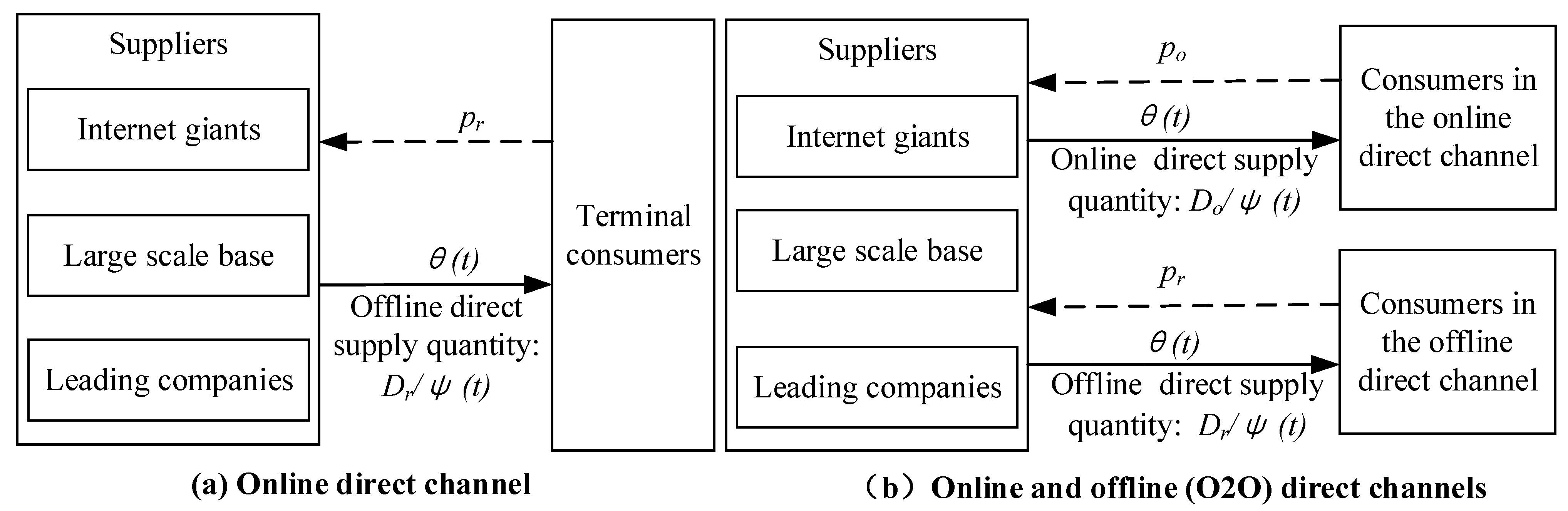
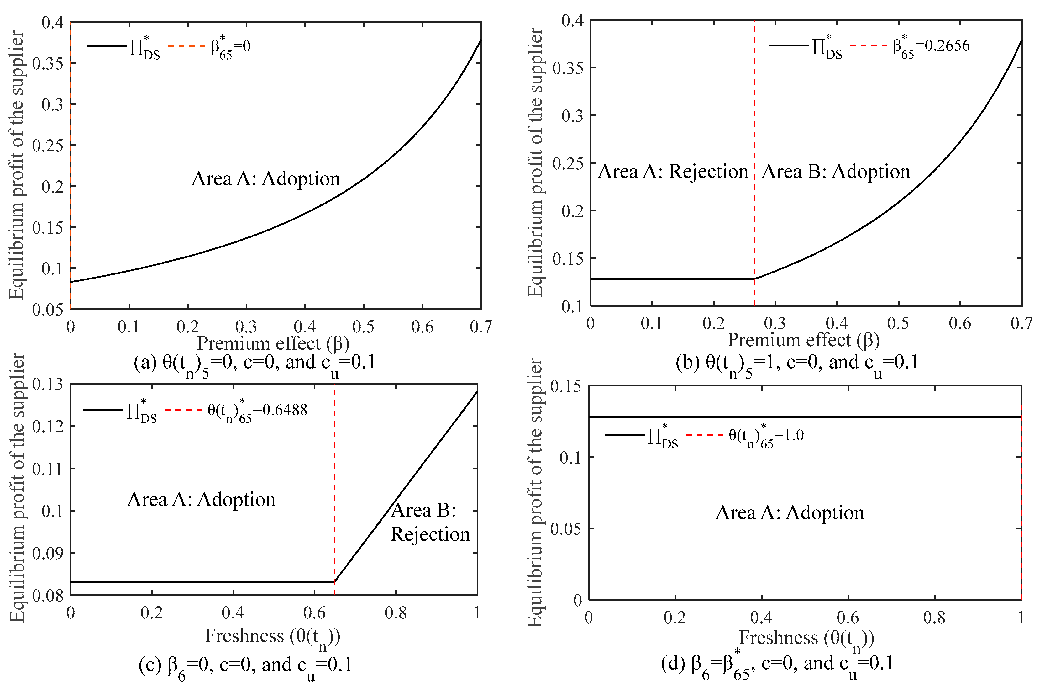
Table 1.
Notations and their related definitions.
| Notation | Definition | Notation | Definition |
|---|---|---|---|
| Parameters concerning the supplier | |||
| S | Supplier | Production cost | |
| Supplier’s profit | Tag cost | ||
| Parameters concerning consumers and market | |||
| Circulation time | Premium effect | ||
| Expiration date | Offline market share | ||
| Premium value | Freshness | ||
| Decay rate | Survival rate | ||
| Deterioration rate | Online direct demand quantity | ||
| Self-price sensitivity | Offline direct demand quantity | ||
| Self-premium sensitivity | Cross-price sensitivity | ||
| Spoilage reduction effect | Cross-premium sensitivity | ||
| Superscript parameters | |||
| L | Lower bound | U | Upper bound |
| B | Bound value | ||
| Subscript parameters | |||
| Without the BTS | Online direct channel | ||
| With the BTS | Offline direct channel | ||
| O | Online direct channel | D | O2O direct channel with differential pricing |
| N | O2O direct channel with non-differential pricing | ||
| Decision variables | |||
| Online direct price | Offline direct price | ||
Disclaimer/Publisher’s Note: The statements, opinions and data contained in all publications are solely those of the individual author(s) and contributor(s) and not of MDPI and/or the editor(s). MDPI and/or the editor(s) disclaim responsibility for any injury to people or property resulting from any ideas, methods, instructions or products referred to in the content. |
© 2024 by the authors. Licensee MDPI, Basel, Switzerland. This article is an open access article distributed under the terms and conditions of the Creative Commons Attribution (CC BY) license (https://creativecommons.org/licenses/by/4.0/).
Share and Cite
MDPI and ACS Style
Zhao, S.; Cao, X. Sustainable Suppliers-to-Consumers’ Sales Mode Selection for Perishable Goods Considering the Blockchain-Based Tracking System. Sustainability 2024, 16, 3433. https://doi.org/10.3390/su16083433
AMA Style
Zhao S, Cao X. Sustainable Suppliers-to-Consumers’ Sales Mode Selection for Perishable Goods Considering the Blockchain-Based Tracking System. Sustainability. 2024; 16(8):3433. https://doi.org/10.3390/su16083433
Chicago/Turabian StyleZhao, Shuai, and Xiaoning Cao. 2024. "Sustainable Suppliers-to-Consumers’ Sales Mode Selection for Perishable Goods Considering the Blockchain-Based Tracking System" Sustainability 16, no. 8: 3433. https://doi.org/10.3390/su16083433
Note that from the first issue of 2016, this journal uses article numbers instead of page numbers. See further details here.