

Analyzing Green Growth Efficiency in China and Investigating the Spatial Effects of Fiscal Decentralization: Case Study of Prefecture-Level Cities

1
School of Economics and Trade, Shandong Management University, Jinan 250300, China
2
School of Public Finance and Taxation, Central University of Finance and Economics, Beijing 102206, China
*
Author to whom correspondence should be addressed.
†
These authors contributed equally to this work.
Sustainability 2024, 16(8), 3408; https://doi.org/10.3390/su16083408
Submission received: 8 March 2024
/
Revised: 7 April 2024
/
Accepted: 16 April 2024
/
Published: 18 April 2024
(This article belongs to the Special Issue Advanced Studies in Economic Growth, Environment and Sustainability)
Abstract
:Due to inadequate resource availability and environmental contamination, the Chinese government has placed a high priority on ecological civilization in recent years. Emphasis has been placed on the environmentally friendly conversion of the economy and the sustainable progress of society. China has established a fiscal decentralization system that divides financial responsibilities between the central and local governments. Due to their proximity advantage, local governments, as agents of the central government, can effectively deliver public services, optimize resource allocation, encourage innovation in green science and technology, and facilitate green growth in the region. However, local governments may exhibit myopic behaviors that impede the sustainable development of the region in their pursuit of regional growth ambitions. Therefore, this paper aims to investigate whether the institutional factor of fiscal decentralization promotes or inhibits the efficiency of green development in China. Using data from Chinese prefecture-level cities between 2010 and 2020, this paper presents the SBM-DDF model to measure the green growth efficiency () in cities. The study then analyzes the spatial impact of fiscal decentralization on using a dynamic panel model and a dynamic SAR model. The empirical results show that China’s green development level has steadily increased in recent years, and reflects climbing pressure and regional differences. Secondly, increasing the vertical fiscal decentralization of local governments promotes growth, while increasing fiscal freedom hinders it. Additionally, fiscal decentralization in neighboring cities also affects local , with spatial spillover effects. Finally, the impact of fiscal decentralization on is spatio-temporally heterogeneous. This paper expands on the research regarding the factors that affect the efficiency of green growth in China, specifically focusing on institutional factors at a theoretical level. Additionally, this paper provides targeted policy recommendations based on the aforementioned findings. These recommendations hold great practical significance for China in improving its fiscal decentralization system and achieving sustainable economic development.
1. Introduction
China’s economy has undergone significant growth since the implementation of economic reforms and opening up. Its Gross Domestic Product (GDP) has surged from RMB 367 billion to RMB 1,260,582 billion between 1978 and 2023, establishing it as the world’s second-largest economy. Nevertheless, this expansion has resulted in a substantial ecological impact. China’s relentless pursuit of economic growth has resulted in major environmental challenges, including the rampant pollution of air and water. These problems pose a direct threat to the health and safety of its citizens and place a substantial strain on the economy [1]. To achieve sustainable economic and ecological development, the Chinese government has proposed five new development concepts—innovation, coordination, greenness, openness, and sharing—with an emphasis on the significance of green development [2]. Green development requires China to abandon its previous model of sacrificing the environment for economic growth and instead adopt a model that prioritizes environmental protection. This entails the reduction in excessive energy use and pollution, as well as the implementation of the green development concept in order to attain a peaceful equilibrium between humans and nature, so assuring enduring and sustainable economic progress. The Chinese government has endeavored to accomplish an ecologically sustainable transformation of the economy. For instance, China has implemented the objective of achieving carbon peaking and carbon neutrality in 2021 as a means to tackle the worldwide problem of increasing carbon dioxide emissions. China will counterbalance carbon dioxide emissions generated from production, everyday life, and other activities through tree planting, energy conservation, and emission reduction, aiming to achieve both positive and negative offsets. China’s objective is to achieve its maximum carbon dioxide emissions by 2030 and then sustain that level [3]. Following a succession of initiatives undertaken by the Chinese government, what is the level of effectiveness in greening China’s economy? Which variables influence the effectiveness of China’s sustainable growth? These matters have incited discourse and reflection among the scholarly community.
The quantifiable progress in enhancing the ecological environment, optimizing resource use, and minimizing waste emissions throughout economic development is known as green growth efficiency [4]. Researchers have created metrics to assess the efficiency of China’s green development and have examined several elements that influence it, such as foreign investment [5], concentration of manufacturing [6], urban growth [7], digital economy, and technical advancements [8]. Nevertheless, the present examination of the influencing elements focuses primarily on economic issues, disregarding the importance of non-economic factors, particularly institutional factors. In order to attain green economic growth, it is imperative to not only mitigate existing pollution but also proactively foster the creation of green products and technologies that encompass both ecological and economic advantages. The production of green products, as well as the implementation of green technologies, often requires significant investment. Market mechanisms, which prioritize efficiency and profits over environmental protection and social responsibility, often fail to adequately compensate for these costs [9,10]. Consequently, government intervention has become essential in fostering green economic growth and mitigating the constraints of the market mechanism. The fiscal decentralization system primarily determines the scope of action for local governments [11]. Fiscal decentralization entails the transfer of authority from the central government to local governments, allowing them to autonomously determine economic management operations and financial matters within their jurisdictions [12]. It is still uncertain whether this increased local government power will impact the effectiveness of green growth. This study will measure the level of green growth efficiency in China cities and investigate the potential influence of fiscal decentralization on it, with a specific emphasis on institutional factors.
This study enhances current research first by employing the slack-based model with directional distance function (SBM-DDF) to assess the efficiency of green growth in prefecture-level cities in China and then analyzing the spatial and temporal features of their green development from a microscopic perspective. Secondly, this article examines the influence of fiscal decentralization as an institutional component on China’s green growth efficiency. For this purpose, we specifically construct a panel model. Additionally, we subsequently develop a spatial auto-regressive (SAR) model to investigate the existence of geographical spillover arising from this impact. Finally, we ultimately expand the static model into a dynamic model to analyze the path-dependent attributes of China’s efficiency in green economic development. This paper presents strategies for local governments to facilitate sustainable development and gives guidance for implementing actions to boost the region’s economy in an environmentally friendly manner. Furthermore, the objective of this study is to improve China’s fiscal decentralization system, providing guidance to local officials on how to effectively combine economic growth and environmental protection. This will optimize the environmental impact of fiscal decentralization and facilitate high-caliber economic growth.
The structure of the paper is as follows: The Section 2 offers a thorough overview of the relevant literature. The Section 3 of the study includes performing theoretical analysis and formulating hypotheses. The Section 4 of the document entails the model’s establishment and the variables’ introduction. The Section 5 examines China’s efficiency in achieving green development, while the Section 6 investigates the influence of fiscal decentralization on it. The Section 7 examines the variation in the impact of fiscal decentralization in different time periods and regions. Finally, we present a brief summary and policy suggestions.
2. Literature Review
This study centers on establishing and quantifying the effectiveness of green growth. David Pearce first introduced the concept of a green economy in 1989. It was defined as a model of economic growth that aims to harmonize the economy and the environment [13,14,15]. Subsequently, scholars have performed studies on green development and the green economy, leading to important advancements in this field. Scholars have started researching ways to evaluate green economic growth by finding indicators that may effectively define and measure the existing status of green development. Currently, the measurement of green economic development can be broadly classified into two methods: the comprehensive index method and the efficiency measurement method. As for the comprehensive index method, the process involves establishing a set of economic efficiency indices and assigning weights to each index. Economic efficiency is assessed by computing the weighted average of the indices. For instance, Liu et al. [16] evaluated China’s green finance and economy using a comprehensive index method based on panel data from 30 provinces between 2007 and 2016. They also established a coupled coordination degree model. Cabernard and Pfister [17] created a multi-regional composite index that describes the development of the global green economy, including indicators such as carbon pressure, water pressure, and biodiversity loss. Mealy and Teytelboym [18] created the Green Complexity Index (GCI) and Green Complexity Potential (GCP) using the composite index method to assess a nation’s capacity to produce environmentally friendly goods. It is believed that the stronger a country’s production capacity for green products, the more favorable its position for green economic development. The efficiency measurement method, which links input data to output indicators to evaluate the economic efficiency of a decision unit, is the second most commonly employed technique. The most frequently utilized strategy for this purpose is the Data Envelopment Approach (DEA). The DEA is a non-parametric method using linear programming to evaluate the relative effectiveness of the decision-making units (DMUs) [19]. Wu et al. [20] utilized the environmental DEA approach to assess green economic efficiency. Regional inequalities in green economic efficiency were found among several regions in China, showing a gradual downward trend. In the research of Shuai and Fan [21], an ultra-efficient DEA model was used to measure China’s green economy efficiency based on provincial panel data. Subsequently, the Tobit model was utilized to confirm how environmental regulations affected the effectiveness of China’s regional green economy. Liu and Dong [4] contended that the national economic growth rate is no longer an appropriate indicator for assessing the quality of economic development and green economic efficiency in China’s current economic climate. The most effective method to evaluate the green economic efficiency of Chinese cities is by utilizing the game-cross-efficiency DEA model.
Fiscal decentralization involves transferring certain tax and spending authorities from the central government to local governments, allowing them autonomy in budget management and economic decision-making. This facilitates a more equitable allocation of power and resources among various tiers of government. The national government uses monetary and fiscal policies to control the macroeconomy, while the local government allocates resources accordingly. They work together to guarantee consistent economic growth and societal progress [11,12,22,23]. Scholars have extensively researched fiscal decentralization, although there is no universally accepted approach for its proper measurement. Measurement methods for fiscal decentralization are typically categorized into three groups: revenue decentralization, expenditure decentralization, and freedom indicators. The revenue decentralization indicator is expressed as the proportion of local government revenue to central government revenue, while the expenditure decentralization indicator is expressed as the proportion of local government expenditure to central government expenditure. These two indicators measure the proportion of fiscal resources available to local governments compared to the central government [24,25,26]. The fiscal freedom index, which gauges how freely local governments can use their financial resources, is calculated as the ratio of fiscal revenue to fiscal expenditure [27,28]. Scholars choose fiscal decentralization indicators for research based on various government perspectives on providing public services.
Academic research on the connection between fiscal decentralization and efficient green growth is currently quite extensive. Scholars have differing opinions on whether fiscal decentralization enhances or hinders the efficiency of green economic development. Some academics believe that fiscal decentralization can promote green economic growth. Song et al. [29], Feng et al. [30], and Yu et al. [31] suggest that optimizing resource allocation, improving local public infrastructure, stimulating enterprise innovation, and promoting the green development of the economy can be achieved through fiscal decentralization. Wang et al. [32] found that fiscal decentralization promotes competitiveness among local governments in technological innovation and other sectors, leading to an enhancement in green total factor productivity. They accomplished this by utilizing provincial data to construct a panel model for empirical analysis. From the perspective of environmental finance, Zhou et al. [33], Ji et al. [34] and Qi et al. [35] discovered that enhancing fiscal decentralization can successfully encourage a city’s green transformation. This is advantageous for conserving energy, reducing emissions, and promoting green development. According to Wang et al. [36], fiscal decentralization can aid local governments in making the transition to a green economy and increase the effectiveness of green economic growth. Nevertheless, fiscal decentralization impacts the growth efficiency of various regions differently. Some researchers contend that fiscal decentralization negatively affects the economy’s green development. Researchers Xin and Qian [37], Fajri et al. [38], Li and Xu [39] and Han [40] have discovered that a drop in the effectiveness of green economic development occurs as local governments’ fiscal decentralization increases. The fiscal decentralization system provides local governments with a level of autonomy. GDP serves as a fundamental criterion for China’s political promotion system. This may result in government personnel participating in chaotic rivalry to attain economic objectives and political aspirations. As a result, local government representatives may choose to implement self-serving tactics to enhance the local economy, leading to increased pollution levels and diminishing the efficacy of green development. Decentralized indicators were generated based on fiscal revenue and expenditure in the studies of De Mello Jr [24] and Song et al. [25]. Revenue decentralization improves local green total factor productivity, but expenditure decentralization reduces it. Zhou and Zhang [26] reached a different conclusion, arguing that revenue decentralization has a minimal effect, whereas fiscal expenditure decentralization has a direct negative impact and spatial spillover effects. Lastly, some academics propose that the effectiveness of economic green development and fiscal decentralization have a non-linear relationship. A negative U-shaped link was discovered between the release of pollutants such as carbon dioxide and fiscal decentralization by Ji et al. [34], Zhang et al. [41], Xia et al. [42] and Wang et al. [43]. Fiscal decentralization, in the short run, enhances regional economic growth and efficiency. However, a rise in fiscal decentralization leads to a decrease in growth efficiency once a specific threshold is reached.
In conclusion, the extensive research on China’s fiscal decentralization, green growth efficiency, and the connections between these two topics has established a strong research foundation for this work. There are still some issues, though. Firstly, the current research on fiscal decentralization and green growth efficiency in China primarily concentrates on the province level, with limited studies investigating the city level. Furthermore, previous studies have used relatively narrow economic output evaluation indicators, whereas economic green development is multifaceted and encompasses a wide range of factors. Thus, a solitary evaluation indication is inadequate. Finally, previous research on the impact of fiscal decentralization on green growth efficiency has not sufficiently included temporal inertia and spatial spillovers. This study examines the relationship between fiscal decentralization and the efficiency of green economic growth implementation in Chinese prefecture-level cities. An evaluation methodology for green growth efficiency is developed utilizing the slack-based model with directional distance function (SBM-DDF) model, a DEA approach that utilizes multi-dimensional indicators. The green growth in Chinese cities will be compared and examined both horizontally and vertically. The dynamic spatial econometric model is utilized to conduct a comprehensive investigation of the impact of fiscal decentralization on the efficiency and diversity of green growth.
3. Theoretical Analysis and Hypothesis
As mentioned by previous research, fiscal decentralization may both promote and inhibit green growth efficiency. This research examines the impact of fiscal decentralization on the efficiency of green growth by analyzing its mechanisms and regional spillover effects. Hypotheses are subsequently suggested.
3.1. Exploring the Mechanism and Hypothesis behind the Positive Impact of Fiscal Decentralization on Green Growth Efficiency
Firstly, the classic idea of fiscal federalism states that local governments may better understand the interests of their constituents and improve the mobility of local government control by implementing a fiscal decentralization system [44]. The central government frequently offers identical products and services for local matters that may not cater to the varied requirements of local populations. This may lead to an ineffective distribution of resources. Local governments have an edge in information dissemination due to their proximity to local inhabitants, allowing for the quick and precise transmission of information [45,46]. Financial liberty is granted to local governments through fiscal decentralization. As a result, they are able to develop environmental management strategies that take into account the opinions and knowledge of the local community regarding the geography and distribution of the area’s natural resources. The outcome is an enhancement in local environmental conditions and the advancement of regional sustainable growth [47]. Efficient urban green development benefits from fiscal decentralization that promotes precise and green governance, leading to the optimal utilization of public resources.
Furthermore, the fiscal decentralization promotion mechanism, which directly piques local governments’ interest in green governance, also has an impact on the effectiveness of regional green development. Fiscal decentralization refers to a vertical management system, wherein a portion of the responsibility over tax revenue and expenditures is delegated to lower levels of government [48,49,50]. The fiscal decentralization concept incorporates a performance evaluation mechanism to motivate local governments to take action. This system allows local government officials to achieve upward promotion based on their performance. Recently, the performance appraisal system in China has started to prioritize green development, giving more importance to indicators like environmental protection and low-carbon development. This actively steers local governments towards green development and enhances the efficiency of regional green economic growth.
Finally, local government investment in science and technology innovation can encourage green growth in the region under the fiscal decentralization system [50,51,52]. Enhanced budgetary autonomy for local government can boost spending on science and technology to enhance the innovation potential of the region and accelerate its green economic growth. The local government’s promotion of scientific and technological innovation can encourage local businesses to actively engage in R&D activities and increase R&D investment. Increased green economic growth efficiency is the result of this.
Accordingly, this paper proposes hypothesis:
Hypothesis 1.
Fiscal decentralization promotes green growth efficiency.
3.2. Exploring the Mechanism and Hypothesis behind the Negative Impact of Fiscal Decentralization on Green Growth Efficiency
Fiscal decentralization can lead to financial resource inefficiency, undermining economic effectiveness and hindering the region’s environmental sustainability efforts. The promotion and appraisal mechanism of fiscal decentralization has induced some local governments to blindly expand and repeat construction to achieve rapid short-term economic growth [53,54]. This has greatly diminished the capacity of local governments to advance green economic development due to the wastage of resources.
Local governments often utilize harsh tax incentives to attract production components from external sources, which may exacerbate the region’s environmental impact and impede the progress of green growth. This is a result of the incentives provided by the policy evaluation process. The fiscal decentralization system provides local governments with special tax relief privileges. Taxes are the main source of government funding. Therefore, expanding the tax base and increasing tax revenue have become the primary methods for local governments to alleviate fiscal pressure. Local governments under financial strain may relax local environmental rules, perhaps leading to an increase in the environmental impact of the region due to the operation of highly polluting industries [55]. Tax competition may alleviate fiscal strain on local governments but does not support local green growth efficiency.
Accordingly, this paper proposes hypothesis:
Hypothesis 2.
Fiscal decentralization inhabits green growth efficiency.
3.3. Mechanism and Hypothesis of the Fiscal Decentralization’s Spatial Spillover Effects on Green Growth Efficiency
Spatial proximity is a stronger indicator of relationship, according to Tobler’s first law of geography [56,57]. Thus, it is necessary to include the spatial impact when studying how fiscal decentralization influences the efficiency of green economic development. Environmental pollution has external impacts, and the management of environmental pollution by municipal authorities can influence adjacent cities. Local governments are accountable for environmental stewardship in their regions as a result of fiscal decentralization. Investing in environmental protection in one area can enhance the environmental quality of neighboring cities. Cities with high green growth efficiency can alleviate environmental pressure on nearby cities, resembling a type of free-riding. This results in beneficial spatial spillovers of green growth efficiency. Local fiscal decentralization affects the efficiency of local green development, which in turn has noteworthy spatial spillovers on the surrounding regions’ green growth efficiency.
Local governments in fiscal decentralization want to extend resource utilization outside their boundaries, vie for intergovernmental resources, and advance regional green development. Governments are currently vying for foreign direct investment as a valuable resource. Foreign investment can positively influence domestic capital and technology, resulting in spillover benefits [58]. Neighboring city enterprises can obtain finance and superior technologies by collaborating with foreign corporations. This will further enhance the efficiency of the region’s green economy.
Accordingly, this paper proposes hypothesis:
Hypothesis 3.
The efficiency of green growth is spatially affected by fiscal decentralization.
Figure 1 summarizes the reasons and regional spillover effects of fiscal decentralization on the efficiency of green growth as stated in this article. Fiscal decentralization can impact green growth efficiency through five pathways, with ’+’ indicating a positive influence and ’−’ indicating a negative effect. Furthermore, there would be spatial linkage and a beneficial spillover effect of green growth efficiency across local governments. This paper will construct econometric models to evaluate the hypotheses mentioned.
4. Methodology and Variables
4.1. Measurement of Green Growth Efficiency
Prior to testing Hypothesis 1, 2, and 3, it is essential to measure the efficiency of green growth in Chinese prefecture-level cities. Academics commonly use DEA to measure green growth efficiency. One of the primary benefits of DEA is its ability to handle multi-input multi-output problems without requiring a specific functional form to be set [59]. Nevertheless, the fundamental DEA approach fails to include unexpected outputs, and it is not possible to quantify slack variables. In order to tackle these problems, researchers have proposed a slack-based model (SBM) that includes unexpected outputs. However, the conventional directional distance function employed in the SBM adopts a radial and directional approach. When assessing slack variables, the utilization of radiality may result in an inflated estimation of efficiency, whereas the directionality fails to consider non-proportional alterations in input and output efficiency simultaneously. Fukuyama and Weber [60] subsequently integrated radiality with the directional distance function, yielding the non-radial and non-directional slack-based model with directional distance function (SBM-DDF). When assessing the efficiency of green growth in Chinese cities, it is essential to take into account both expected outcomes, such as economic benefits, and unexpected outcomes, such as pollution emissions. Furthermore, it is crucial to avoid any inaccuracies in the calculated efficiency results caused by excessive inputs or insufficient outputs. Thus, this research employs the SBM-DDF model to establish the production technology frontier, incorporating all prefecture-level cities in China as decision-making units (DMUs).
Once the production technology frontier has been established, it is customary in academia to employ the Malmquist–Luenberger index to assess the efficiency of a DMU. However, the Malmquist–Luenberger index is problematic due to concerns related to unsolved linear programming and non-transferability. Thus, Oh [61] suggests the creation of the global Malmquist–Luenberger (GML) index, which relies on the global production technology frontier established using global data. The GML index ensures consistent productivity assessments over time and prevents problems with unsolvable linear programming. This method has emerged as the predominant approach for assessing green growth efficiency in recent years.
To summarize, this paper utilizes the SDM-DDF model and applies the GML index to measure the efficiency of green development in 271 prefecture-level cities in China. (Due to different administrative levels, four municipalities directly under the central government—Beijing, Tianjin, Shanghai, and Chongqing—are excluded from this paper. Due to missing data, Lvliang, Chaohu, Sansha, Danzhou, Bijie, Tongren, Pu’er, Lhasa, Shigatse, Chamdo, Linzhi, Shannan, Nagchu, Haidong, Hainan, Zhongwei, Turpan, Hami, Mudanjiang, Laiwu, Jinchang, Tianshui, and Yinchuan are excluded from this paper. Due to different statistical calibers, this article excludes Hong Kong, Macao, and Taiwan.).
4.1.1. SBM-DDF Model
Assume that there are N input indicators x, M expected output indicators y, and K unexpected output indicators b in the model, denoted as , and . Then, represents the vector of inputs and outputs for the i region in the t year. is the direction vector representing input compression, expected output increase and unexpected output expansion, respectively. represents the slack variables of inputs and outputs. The SBM-DDF model for the i region is denoted as in Equation (1):
4.1.2. Global Malmquist–Luenberger Index
The Global Malmquist–Luenberger Index is calculated as presented in Equation (2).
In Equation (2), is green growth efficiency, which is denoted by in this paper. Global technical change () and global efficiency change () are the two components that make up the . and denote the current and global SBM directional distance functions constructed based on the non-radial and non-directional methods, respectively. The efficiency of green growth is enhanced when the index is greater than one. If it is less than one, it suggests that green growth is becoming less efficient. If it equals one, it shows a stable level of green growth efficiency.
4.1.3. Data Processing and Indicator Selection
According to the Cobb–Douglas production function, the city uses labor and capital as production input components when it functions as a DMU [62]. Based on the city’s yearly investment in fixed assets, the capital stock is calculated using the perpetual inventory method to estimate the capital input factor. The number of employees in workplaces at the end of the year is the labor input factor. The research presents a novel input indicator that takes energy consumption into account. This is because energy use is the primary source of pollution in the city’s production processes. In summary, labor, capital, and energy are the defined input indicators of the model.
Regarding the output indicators, as a growth in output is the desirable result of urban production, the real GDP level of the cities in the current year is selected as the expected output of the SBM-DDF model. Additionally, pollutant emissions are the undesired results of cities during green production. The availability of data from prefecture-level cities indicates that emissions of wastewater, sulfur dioxide, smoke and dust are typically employed as indications of the unexpected output of the city [63,64]. However, carbon emissions are not included in these metrics. As previously noted, China has worked very hard to reach carbon neutrality and the carbon peak, and carbon emissions should also serve as an unexpected output indicator to demonstrate China’s green economic progress. Therefore, this research objectively evaluates wastewater, sulfur dioxide, smoke and dust, and carbon emissions as measures of unanticipated output to reflect environmental pollution caused by economic development. Carbon emissions data for each prefecture-level city in China are categorized into three scopes. Scope I encompasses the direct carbon emissions originating from activities within the city’s jurisdiction, including transportation, buildings, and industrial production processes. Scope II includes indirect carbon emissions originating from sources such as purchased power, heating, and cooling that are utilized to fulfill urban consumption needs but are located outside the city’s control. Scope III pertains to indirect emissions resulting from activities within the city but occurring outside, such as transportation. Table 1 provides detailed information on the meaning and specific calculations of each input and output indicator.
4.2. An Examination of Fiscal Decentralization’s Effect on GGE
4.2.1. Dynamic Panel Regression Model
In order to test Hypotheses 1 and 2, this paper presents the following model in Equation (3) to analyze the impact of fiscal decentralization on . The dynamic panel regression model is established by including with a one-period lag as an explanatory variable to account for the long-term character of green economic development:
In Equation (3), denotes the current green growth efficiency of the prefecture-level city i. denotes the lagged one-period level of . denotes the level of fiscal decentralization, and is the core explanatory variable. denotes the control variable and is a constant term. is the unobservable time effects and is the unobservable individual effects. At last, denotes a random disturbance term.
4.2.2. Regression Variable Selection and Descriptive Statistics
This article uses two indicators to assess fiscal decentralization. The initial indicator assesses the distribution of resources between the central government and local governments. The variable is utilized, with a higher value indicating a greater degree of decentralization. The second indicator of fiscal decentralization is defined as the ratio of fiscal revenue to fiscal spending when considering the distribution of local government fiscal resources. The variable quantifies the level of decentralization, where larger values signify increased autonomy in utilizing fiscal resources.
This paper looks at studies of Song et al. [29], Chen et al. [65], Wang et al. [66], Qiu et al. [67] and Wang et al. [68], and then chooses seven control variables for the dynamic panel regression model. These are as follows: openness to foreign countries (), industrial structure (), economic development (), scientific and technological development (), education level (), import dependence (), and export dependence (). Table 2 presents the definitions, calculation methods, and data sources for all variables. Table 3 displays the descriptive statistics for all variables.
4.3. Spatial Econometric Model
Econometric models typically presume that variables or indicators are independent. However, in reality, economic data often exhibit spatial relationships, particularly in the context of green growth efficiency. Green economies in many locations are not just unbalanced but also interconnected through geographical links. This study employs a spatial econometric model to examine the influence of fiscal decentralization on green growth efficiency in Chinese cities and to assess the validity of Hypothesis 3. Typically, spatial econometric models can be categorized into three different categories. The first category is the spatial auto-regressive model (SAR), which investigates whether the dependent variable in one location is influenced by that in a neighboring region, indicating a spatial spillover effect of dependent variable. The second category is the spatial error model (SEM), which examines whether the dependent variable in a particular region is influenced by the error shocks in nearby regions, indicating the presence of geographical spillovers in the error term. The spatial Durbin model (SDM), belonging to the third category, incorporates a spatial lag term for the independent variables, which is an addition to the first two categories. Before starting the spatial empirical investigation, it is essential to select the appropriate geographic economic model from the SAR, SEM and SDM model. Based on the LM test, Robust-LM test, Hausman test and LR test conducted subsequently in this paper, the SAR model with individual fixed effects is used in this study. The SAR model is expanded to a dynamic SAR model by incorporating the lag term of to consider the time inertia of the dependent variable. The dynamic SAR model is shown in Equation (4):
Every item in Equation (2) has the same meaning as it has in Equation (1). The spatial link between nearby cities is represented by the spatial weight matrix . This paper aims to comprehensively measure the spatial correlation between cities, taking into account the dual influence of economy and geography. To achieve this, we have chosen to construct a spatial weight matrix based on four dimensions. The specific spatial weight matrix is constructed as follows:
- Geographic neighboring weight matrix . The geographic neighboring weight matrix uses a single binary rule to determine spatial relationships. For two spatial units, the value is one if the two units are adjacent, and zero otherwise. The formula is:
- Economic distance weight matrix . In regions with similar economic levels, fiscal balance, green technology, and openness to the outside world are also similar. Therefore, their efficiency in green economic development should also be closer. The essence of economic distance is the economic gap between two cities. In this paper, we first take the absolute number of the difference between the average per capita GDP () of the two cities from 2010 to 2020, and use the inverse of its absolute number to construct the economic distance weight matrix. Its formula is:
- Geographic distance weight matrix . In this paper, firstly, the geographic distance between each prefecture-level city government needs to be determined through their latitude and longitude. Then, it takes the inverse of the square of and uses this to construct the geographic distance spatial weight matrix. Its expression is:
- Economic geography nested matrix . All of the above weight matrices describe the possible spatial correlations among cities from only one perspective. In this research, an economic geography nested matrix is constructed in order to analyze the spatial relationships of cities in detail. This weight matrix not only contains the role of spatial spillover generated by the geographical location between different regions but also contains the spatial relationships generated by various economic factors. The construction process is as follows:
5. Temporal and Spatial Analysis of
5.1. Time Trend Analysis of
The study employed data from 2010 to 2020 to calculate the of 271 Chinese prefecture-level cities between 2011 and 2020 using Matlab. The was broken down into and . Figure 2 displays the temporal evolution of the mean value of the three indicators across all cities in the study. Figure 2 features a vertical axis with an origin at one. An index number above one signifies increased green growth in the current year compared to the previous year, together with enhanced efficiency in green growth. If the score is less than one, it suggests a decrease in the effectiveness of green growth. Between 2011 and 2014, China’s and its decomposition indicators remained below one, indicating a decrease in efficiency. Since 2015, China’s and decomposition indices have been steadily growing, showing an overall positive trend. In 2019, there was a significant decrease in the indicators, possibly due to the adverse impact of COVID-19 on the growth of the local green economy. In 2020, the indicators displayed signs of recovery. The index rose from 0.987 in 2011 to 1.005 in 2020, showing a total gain of about 0.018. The , which assesses technical change, was below one from 2011 to 2020 and over one in the remaining six years, leading to a total gain of around 0.017 in its value. Figure 2 demonstrates that the patterns of and are comparable, suggesting that China’s green economic advancement relies primarily on technological advancements. denotes variations in technical efficiency, being below one in four years and above one in six years from 2011 to 2020. However, its expansion was sluggish, indicating that China’s overall green economic effectiveness depends less on technology efficiency, which still needs enhancement.
China is a vast country with numerous prefecture-level cities. All sample cities are categorized into three parts, Eastern, Central, and Western China, to more accurately represent regional variations. Figure 3 displays the temporal evolution of the index for each region and the average level from 2011 to 2020. Figure 3 shows that the growth trend is similar throughout the eastern, central, and western areas. The value was below one between 2011 and 2014 and mostly over one after 2015, aligning with the national average. The efficiency values in the eastern and central regions experienced the most rapid growth and were nearly equal when comparing their average levels. The efficiency values in the western region consistently fell behind those in the eastern and central regions, showing little growth in only a few years. The data indicate that the efficiency of green economic development is relatively balanced across the three regions of China, with the western region, which lags behind in economic development, being slightly less efficient. Hence, when analyzing the effect of fiscal decentralization on in this study, it is important to consider regional characteristics for heterogeneity analysis.
5.2. Regional Characteristics Analysis of GGE
This study analyzes data from the prefecture-level city to focus on a micro perspective rather than presenting data at the national or regional level. In order to visualize the changes in and the spatial distribution characteristics of each city, this paper presents the of the Chinese sample cities in each year in Figure 4. The indexes for 2019 are not presented here, as they are not representative due to the impact of external shocks such as COVID-19. In addition, Hong Kong, Macao, Taiwan, certain cities in Tibet, Xinjiang, and other provinces are not included in the graph due to a lack of relevant data. They are represented as non-study areas and colored white. Figure 4 shows that the darker green shade corresponds to a larger value, whereas the lighter shade implies a lower value. Figure 4 illustrates that the level of greenery in Chinese metropolitan areas has progressively intensified over time, suggesting a rise in green growth efficiency. The intensification of the green color originated in central cities and has already spread to northeastern cities, as well as coastal urban areas in the east and south. The 2018 and 2020 graphs indicate a more equitable distribution of among central and eastern cities, reflecting China’s more balanced green economic growth. The eastern and central regions, comprising the provinces of Heilongjiang, Liaoning, Fujian, Zhejiang, Guangdong, Hubei, and Hunan, have higher efficiency levels as seen by the darkest hues in Figure 4. On the contrary, the majority of the western regions are less efficient, with the exception of a few cities, such as the province of Qinghai. There is an uneven distribution of among cities in the western region.
To demonstrate the spatial distribution of indicators in prefecture-level cities at the micro level more clearly, this paper includes a plot of the average in each city from 2011 to 2020 in Figure 5. A darker green tint signifies a greater value. The plot illustrates that the is elevated in the eastern and central regions, displaying a more equitable distribution. The western part displays a pale green hue that fades towards the northern and southern areas. Inland cities, however, appear darker in green. The unequal progress of is a notable concern in the western area.
6. Econometric Model Results Analysis
6.1. Dynamic Panel Regression Results Analysis
A Hausman test was performed on the static panel model, and at a significance level of 1%, the initial hypothesis of Hausman test was rejected. This outcome aligns with the fixed effects model, supporting the use of the fixed effects form. The decision to choose individual fixed effects was based on their better F-statistics compared to temporal fixed effects and both fixed effects. Table 4 displays the results of both static and dynamic panel regression models. Models (1) and (3) are static models that use and as indicators of fiscal decentralization, respectively. Models (2) and (4) are transformed into dynamic models by incorporating the lagged one-period explanatory variable L. into models (1) and (3). The dynamic model outperforms the static model with a higher value, providing a more comprehensive explanation for the variations in green growth efficiency. The dynamic model can address the issue of model endogeneity [69].
All the coefficients are considerably negative in models (2) and (4) from Table 4. Increasing the city’s green economic growth efficiency in the past leads to a loss in efficiency in the present. The reason for this may be that the indicator measures the change in the efficiency of green development in the current period relative to the previous period. If the rise of in the previous era was substantial, the present period can experience development pressure and struggle to sustain the initial level. It indicates that instead of path dependence, there could be increasing pressure on the city’s green growth.
The coefficient of in model (2) is 0.047, and it is statistically significant at the 1% level. When the local government has more financial resources than the provincial and federal governments, it can effectively utilize its informational advantage to enhance green economic growth through promotion mechanisms and increased R&D. The positive impacts surpass the negative effects through channels including resource wastage and tax competitiveness, confirming Hypothesis 1. Nevertheless, model (4) shows a notably negative coefficient for , supporting Hypothesis 2 and indicating that fiscal decentralization may hinder sustainable economic growth. When budgetary pressure on local governments reduces, their budget limits are relaxed, enabling more funds to be committed towards infrastructure projects or favorable tax schemes. However, rather than aiding the local economy in a sustainable manner, this may lead to the wastage of resources due to redundant construction projects or the attraction of energy-intensive and polluting enterprises through tax incentives. In summary, improving fiscal decentralization in terms of measuring the degree of decentralization at higher levels of government can promote green growth efficiency. On the contrary, increasing fiscal decentralization in terms of measuring the degree of freedom of local governments to use their own fiscal resources will reduce green growth efficiency.
Finally, models (2) and (4) indicate that industrial structure, economic development, and education level are significant influencing factors. The coefficients consistently exhibit positive or negative values across all models, indicating the stability of the estimates for the control variables. The positive coefficient of industrial structure suggests that transitioning the economy from primary to secondary and tertiary industries will encourage regions to adopt energy-saving and emission reduction practices, thereby enhancing green growth efficiency. Increasing economic development has a detrimental effect, as it exacerbates issues related to resource utilization and pollution emissions, thereby impeding the progress of green economic development. A beneficial effect on education level is also noted. The higher the education level in a population, the easier it is to promote the green notion of energy conservation and emission reduction, therefore aiding the region’s green economic development.
6.2. Dynamic Econometrics Results Analysis
To test Hypothesis 3, this paper establishes a spatial econometric model to verify the spatial spillover effect of fiscal decentralization on green growth efficiency. Firstly, we conduct a spatial correlation test of the dependent variable and the two fiscal decentralization indicators. The dynamic SAR model will be created next.
6.2.1. Moran’s I Analysis
The Moran’s I index is utilized to test the spatial correlation among variables. Moran’s I includes both global and local indices. The global Moran’s I indicates whether all prefecture-level cities have spatial correlation in a certain year from a macro level. If the index is above zero, it indicates a positive spatial correlation in the data. Greater values indicate a stronger spatial association. When the index is less than zero, it indicates that the data are spatially negatively correlated. A smaller value indicates a larger spatial difference. A global Moran’s I value of zero indicates that the data are spatially random [70,71]. Local Moran’s I shows the correlation distribution of prefecture-level cities at the micro level. Local Moran’s I does not have the same limitations on its range as global Moran’s I. A scatter plot is typically utilized to depict spatial association. The four quadrants of a scatter plot can be used to assess the relationship between one area and its adjacent cities. A distribution in the first quadrant indicates high values for both the area and its surrounding areas. Conversely, a distribution in the third quadrant indicates low values for both the area and its surrounding areas. Therefore, if the scatter is mainly distributed in quadrants one and three, it indicates a positive spatial correlation. If the distribution is in quadrants two and four, it signifies a negative spatial correlation [70,72,73].
Table 5 displays the global Moran’s I and p-values for , , and from 2011 to 2020. Matrix depicts the spatial correlation of cities with regard to economic and geographical integration, providing a more accurate representation of the proximity of city linkages. Table 5 exclusively presents the regression outcomes using matrix . Table 5 shows that, except for 2012 and 2018, when global Moran’s I is not significant, shows positive spatial correlation in all years. Both fiscal decentralization measures, and , have p-values < 1% in all years, suggesting a strong positive geographical association. Additional matrices provide substantial positive spatial correlation, justifying the establishment of a spatial econometric model.
Figure 6 displays the scatter plots of local Moran’s I for , , and in 2011 and 2020, using matrix . In both years, the majority of prefecture-level cities show local Moran’s I values spread in quadrants one and three. The green growth efficiency and fiscal decentralization of cities are characterized by either high–high or low–low aggregation. The results of local spatial correlation can indicate the suitability of using a spatial econometric model.
6.2.2. Dynamic SAR Model Results Analysis
The analysis of spatiality indicates significant spatial spillover effects of both the dependent variable and the core explanatory variables in this paper. Table 6 displays the previous examinations for the spatial econometric model configuration. Based on the LM test and robust-LM test, the model disproves the hypothesis that it lacks a spatial lag term in the dependent variable and confirms the hypothesis that it lacks a spatial lag term in the error term. In Table 6, the Hausman test suggests that a fixed effects model is the appropriate choice. Furthermore, the LR test confirms that the fixed effects are individually fixed. Therefore, a dynamic SAR model is established to explore the direct effect of fiscal decentralization on as well as the spatial spillover effect. The regression results are displayed in Table 7. Models (5)–(8) utilize as the fiscal decentralization indicator, depicting the dynamic SAR model across four distinct spatial matrices. Models (9)–(12) utilize as the fiscal decentralization indicator.
Initially, the results show that the lagged period of the dependent variable remains consistently negative throughout the four spatial matrices. This suggests an increasing strain on the efficiency of local green growth, in line with the findings of the dynamic panel model regression. and denote the spatially lagged terms of the for the current and previous eras, respectively. The study shows how the green growth efficiency of nearby cities in both the present and former periods affects the influence of this city in the current period. As shown in Table 7, the coefficients of the two variables exhibit a strong positive relationship, indicating that improvements in nearby regions benefit the local area’s . This effect is particularly evident in the current and lagged periods. Green economic development can enhance local efficiency by facilitating the transfer of technology and finance from surrounding regions. The positive regression coefficient aligns with the prior conclusion drawn from Moran’s I test and indicates the suitability of employing the dynamic SAR model in this study. Secondly, except for model (3), the coefficients of in the other models are statistically significant at a 5% level and positive. The coefficients of are statistically significant at a 1% level and are negative, confirming Hypotheses 1 and 2. An increase in local government vertical fiscal decentralization enhances the region’s green growth, even when accounting for spatial spillover effects. Conversely, an increase in the degree of fiscal freedom leads to a decline in green development. Lastly, the impacts of and are positive and consistent in several models, like the dynamic panel model. Urban areas boost green growth efficiency by shifting towards secondary and tertiary sectors, and higher education levels among citizens also contribute to this effect. The coefficients of the variable are statistically significant in models (5)–(8) but not in models (9)–(12). Their constant negativity is in line with the findings of dynamic panel regression.
Table 7 displays the coefficients of and , but their magnitude does not directly reflect their influence on . The fiscal decentralization of nearby regions affects the of those regions, which in turn has an impact on the neighborhood through spatial spillovers. It is crucial to consider both the effects on neighboring areas and local-to-local interactions when analyzing how fiscal decentralization would affect . This study uses the differential technique to assess the regression coefficients of the dynamic SAR model to illustrate the diverse effects of fiscal decentralization on , considering the dynamic changes between the long and short terms. The impacts of fiscal decentralization on are divided into long- and short-term direct, indirect, and total effects, as shown in Table 8. The direct effect shows how the city variables affect the city’s , while the indirect effect shows how the adjacent city variables impact the city’s . This study solely displays the regression outcomes of matrix , namely models (8) and (12), for the purpose of decomposition. Additionally, since the results of and are more robust, this paper also decomposes their total impact effects. The short-term effects of fiscal decentralization outweigh the long-term effects as Table 8 demonstrates. The impact of institutional factors on green growth efficiency diminishes gradually over time. The positive effects of on , both short- and long-term, indicate that local green economic development benefits from the enhanced vertical decentralization of local governments in the area. The negative impacts of might hinder local green economic growth by reducing fiscal pressures and relaxing budgetary limits in local and nearby areas. The analysis confirms Hypothesis 3 by showing the significant spatial spillover impacts of fiscal decentralization on . The significant indirect effects of both and in the long and short terms demonstrate how nearby industrial upgrading and education improvement increase the effectiveness of local green development.
7. Heterogeneity Analysis
This section of the article will carry out a heterogeneity test in time and place to examine if the influence of fiscal decentralization on the efficiency of green economic development is altered by varying development time periods and spatial distributions of the .
7.1. Tests for Temporal Heterogeneity
was below one until 2014, and then it consistently rose to above one after 2015 as previously discussed. displays distinct traits in the two time periods. To examine the impact of fiscal decentralization in different time periods, this paper divides the sample time period into two parts: 2011–2014 and 2015–2020. Dynamic SAR models are established for each period. Table 9 and Table 10 present the regression results for and , respectively.
Table 9 illustrates that the adverse effects of in the previous period notably diminished after 2015, suggesting a reduction in the growing strain during the period of enhancing green growth efficiency. The existence of time inertia and the path dependence of favorable factors, such as green development technology, may be the reasons for this. This enhances the ongoing enhancement of green economic efficiency. is significantly positive in all periods, suggesting that there are spatial spillover effects of fiscal decentralization on in both periods, in line with Hypothesis 3. The level has markedly risen since 2015, suggesting that an enhancement in green growth efficiency will lead to a more pronounced spillover effect. The most noticeable observation in Table 9 is that the variable is not statistically significant for the years 2011–2014, which contradicts Hypothesis 1. Conversely, the variable exhibits a notably upward trend from 2015 to 2020, which aligns with Hypothesis 1. An enhanced vertical decentralization of fiscal resources by local governments has a stronger beneficial effect on when green growth efficiency increases.
Similar to Table 9, Table 10 also indicates a decline in during the latter period, suggesting a decrease in the climbing pressure. Furthermore, the variable exhibits a substantial positive spatial correlation, confirming the validity of Hypothesis 3 in both time periods. The spatial effects of fiscal decentralization become more pronounced as the level of rises during the period of 2015–2020. Table 10 demonstrates that had a notably adverse effect during the period of 2011–2014, aligning with Hypothesis 2. Nevertheless, the impact is no longer statistically significant for the period of 2015–2020, which contradicts Hypothesis 2. Local governments’ inefficient economic intervention ceases when fiscal restrictions are loosened due to a rise in the efficiency of green growth. As a result, local governments will make more rational use of fiscal funds to support the green development of the local economy.
7.2. Tests for Regional Heterogeneity
The study conducts sub-group regression analysis utilizing models (8) and (12) to examine the impact of fiscal decentralization on in Eastern, Central, and Western China. The selected spatial matrix is . The empirical regression results for these regions are displayed in Table 11.
Table 11 demonstrates that the eastern, central, and western regions share a number of characteristics. All time lag components are notably negative, whereas spatial lag terms are positive, suggesting increasing pressure and spatial spillover. The coefficient of is significantly positive, whereas the coefficient of is strongly negative. The findings of the subarea regression and the overall sample regression align. Table 11 shows regional differences in fiscal decentralization coefficients, with the eastern region having the highest values of 0.044 and −0.032. The eastern region’s high level of economic development may lead to increased vertical decentralization and autonomy in fiscal resource allocation. Local governments in the eastern region can effectively stimulate technological innovation, reduce pollutant emissions, improve the economic efficiency of enterprises, and promote green economic development by competing for talent, increasing investment in scientific research, and opening up to the outside. Fiscal decentralization can greatly influence green growth efficiency through various positive and negative pathways. While not appreciably different from one another, the values of the two fiscal decentralization coefficients in the central and western regions are slightly lower compared to the eastern region. These two regions may have a weaker influence on due to their lower economic development and fiscal autonomy. In comparison to the eastern and central regions, Table 11 also demonstrates that the western region has substantially fewer geographical spillovers. This is evident from the lowest coefficients and the lack of significant lagged period results. This may be due to the western region’s bigger urban area, lower enterprise density, and less frequent transfer of resources and technology compared to the eastern and central regions. Consequently, there is a slight geographical connection among cities, which is notably weaker, especially with a one-period delay.
8. Conclusions and Policy Recommendations
This paper proposes research hypotheses derived from theoretical studies and evaluates the green growth efficiency of 271 prefecture-level cities in China from 2011 to 2020 using the SBM-DDF model. The regional and temporal distribution properties of are next analyzed. This research utilizes a dynamic panel model and a dynamic SAR model to analyze the direct, indirect, and various effects of fiscal decentralization on green growth efficiency. According to the study, has been consistently increasing since 2015, with higher levels observed in the eastern and central regions compared to the western region. Moreover, the growth of has a radial diffusion pattern, starting in the middle area and then expanding to the eastern area. Green growth in the eastern and central regions is more evenly distributed, whereas the western region has disparities in development. The increase in reflects rising pressure and shows significant regional connections and positive spatial spillover. An empirical investigation indicates that higher vertical fiscal decentralization in local governments enhances green growth efficiency, whereas increased freedom in local government fiscal decisions impedes it. This effect shows substantial variation over time and across various parts of China. The paper’s findings are significant for improving China’s existing fiscal system, advancing regional green development, and ultimately attaining sustainable economic growth. The study’s findings suggest the following policy recommendations:
Firstly, the reform of fiscal decentralization should be enhanced. The paper’s empirical findings indicate that greater fiscal autonomy for local governments hinders the development of the green economy, but they do not signify a disapproval of the fiscal decentralization system. China’s economic growth following its reform and opening up has been significantly boosted by fiscal decentralization. Continuous improvement of relevant reforms is essential to strengthen fiscal decentralization in accordance with the current historical development period and the demands of the new era. To begin with, the revenue authority reform should be reinforced to prevent local governments from inappropriately influencing the economy to boost fiscal revenue. Additionally, the central government should restrict the local government’s spending authority in productive sectors to prevent their support for high-pollution and high-energy-consumption companies. This will assist the fiscal department in returning to its focus on servicing the public. At last, there should be an improvement in budget performance management. To enhance the efficiency of financial fund utilization, local government behavior variability should be minimized through the regulation of their economic conduct.
Secondly, although the empirical study in this paper suggests that an increase in the degree of vertical fiscal decentralization by local governments can significantly enhance green growth efficiency, there is still room for improvement in this system, particularly in the supporting system of fiscal decentralization. On one hand, the central government should create a thorough assessment system and advancement process for local government personnel. Together with GDP measures, this system ought to consider the potential for economic growth, the costs to the environment, and the need to standardize the financial practices of local governments. Through the use of a fair evaluation system for official advancement, the goal is to inspire officials to actively enhance the standard of the green economy. The national government should enhance local environmental regulation and accountability. Local governments should analyze green performance and define the specific powers and environmental protection duties of each government level.
Thirdly, a system for coordinated green development is required. The distribution patterns of the assessed in this study reveal a spatial imbalance in China’s green growth efficiency, with higher levels in the eastern and central regions and lower levels in the western areas. The central government should improve the coordinated development mechanism by utilizing macro-control to coordinate green production levels, thus enhancing the productivity of each region. On the one hand, promoting the reasonable flow of resources, personnel, and technology between regions is crucial. The eastern area should implement technical support measures to enhance the transfer of resources from the western region to the eastern region to effectively enhance across the country. On the other hand, promoting intra-regional factor movements and coordinating the development of internal areas is crucial. Local governments should increase their involvement and cooperate with adjacent cities to resolve any shortcomings.
Finally, policies should be customized to fit local conditions. The heterogeneity analysis in this research reveals substantial variations in the influence of fiscal decentralization on the efficiency of green growth among different cities in China. It is crucial to take into account the varying economic development statuses and distinct location characteristics of each city in order to identify a starting point for development and work towards minimizing inter-regional disparities. Local governments should refrain from adopting a standardized approach to policy-making and instead create policies that are customized to their unique development circumstances. They should maximize the advantages of information and encourage the improvement of green growth efficiency.
This article examines the impact of fiscal decentralization as an institutional influencing factor on the efficiency of green development in Chinese cities. However, it is important to note that there are other institutional factors, such as environmental regulation, that may also influence this efficiency. Furthermore, this study only focuses on fiscal decentralization and does not consider the influence of financial decentralization, another significant decentralization system in China, on green growth efficiency. Future research should provide a more comprehensive analysis of how fiscal decentralization, financial decentralization, and their combination affect the efficiency of green growth in Chinese cities.
Author Contributions
Conceptualization, Y.L.; Methodology, L.B.; Software, L.B.; Validation, Y.L.; Formal analysis, L.B.; Resources, Y.L.; Data curation, Y.L.; Writing – original draft, L.B.; Writing – review & editing, Y.L. and L.B.; Visualization, L.B. All authors have read and agreed to the published version of the manuscript.
Funding
This research received no external funding.
Institutional Review Board Statement
Not applicable.
Informed Consent Statement
Not applicable.
Data Availability Statement
Data are contained within the article.
Conflicts of Interest
The authors declare no conflicts of interest.
References
- Liang, H.; Zhang, Y.; Liang, H.; Zhang, Y. Green development: Belt and Road is global and rational. In The Theoretical System of Belt and Road Initiative; Springer: Singapore, 2019; pp. 35–38. [Google Scholar]
- Li, D.; Zeng, T. Are China’s intensive pollution industries greening? An analysis based on green innovation efficiency. J. Clean. Prod. 2020, 259, 120901. [Google Scholar] [CrossRef]
- Liu, Z.; Deng, Z.; He, G.; Wang, H.; Zhang, X.; Lin, J.; Qi, Y.; Liang, X. Challenges and opportunities for carbon neutrality in China. Nat. Rev. Earth Environ. 2022, 3, 141–155. [Google Scholar] [CrossRef]
- Liu, Y.; Dong, F. How technological innovation impacts urban green economy efficiency in emerging economies: A case study of 278 Chinese cities. Resour. Conserv. Recycl. 2021, 169, 105534. [Google Scholar] [CrossRef]
- Zhao, P.J.; Zeng, L.e.; Lu, H.Y.; Zhou, Y.; Hu, H.Y.; Wei, X.Y. Green economic efficiency and its influencing factors in China from 2008 to 2017: Based on the super-SBM model with undesirable outputs and spatial Dubin model. Sci. Total Environ. 2020, 741, 140026. [Google Scholar] [CrossRef]
- Yuan, H.; Feng, Y.; Lee, C.C.; Cen, Y. How does manufacturing agglomeration affect green economic efficiency? Energy Econ. 2020, 92, 104944. [Google Scholar] [CrossRef]
- Lin, B.; Zhou, Y. Measuring the green economic growth in China: Influencing factors and policy perspectives. Energy 2022, 241, 122518. [Google Scholar] [CrossRef]
- Li, J.; Chen, L.; Chen, Y.; He, J. Digital economy, technological innovation, and green economic efficiency—Empirical evidence from 277 cities in China. Manag. Decis. Econ. 2022, 43, 616–629. [Google Scholar] [CrossRef]
- Elshamy, H.M.; Ahmed, K.I.S. Green fiscal reforms, environment and sustainable development. Int. J. Appl. Econ. Financ. Account. 2017, 1, 48–52. [Google Scholar] [CrossRef]
- Gao, Q.; Chen, H.; Zhao, M.; Zeng, M. Research on the Impact and Spillover Effect of Green Agricultural Reform Policy Pilot on Governmental Environmental Protection Behaviors Based on Quasi-Natural Experiments of China’s Two Provinces from 2012 to 2020. Sustainability 2023, 15, 2665. [Google Scholar] [CrossRef]
- Lin, J.Y.; Liu, Z. Fiscal decentralization and economic growth in China. Econ. Dev. Cult. Change 2000, 49, 1–21. [Google Scholar] [CrossRef]
- Hung, N.T.; Thanh, S.D. Fiscal decentralization, economic growth, and human development: Empirical evidence. Cogent Econ. Financ. 2022, 10, 2109279. [Google Scholar] [CrossRef]
- Ehresman, T.G.; Okereke, C. Environmental justice and conceptions of the green economy. Int. Environ. Agreem. Politics Law Econ. 2015, 15, 13–27. [Google Scholar] [CrossRef]
- Loiseau, E.; Saikku, L.; Antikainen, R.; Droste, N.; Hansjürgens, B.; Pitkänen, K.; Leskinen, P.; Kuikman, P.; Thomsen, M. Green economy and related concepts: An overview. J. Clean. Prod. 2016, 139, 361–371. [Google Scholar] [CrossRef]
- Pan, W.; Pan, W.; Hu, C.; Tu, H.; Zhao, C.; Yu, D.; Xiong, J.; Zheng, G. Assessing the green economy in China: An improved framework. J. Clean. Prod. 2019, 209, 680–691. [Google Scholar] [CrossRef]
- Liu, N.; Liu, C.; Xia, Y.; Ren, Y.; Liang, J. Examining the coordination between green finance and green economy aiming for sustainable development: A case study of China. Sustainability 2020, 12, 3717. [Google Scholar] [CrossRef]
- Cabernard, L.; Pfister, S. A highly resolved MRIO database for analyzing environmental footprints and Green Economy Progress. Sci. Total Environ. 2021, 755, 142587. [Google Scholar] [CrossRef] [PubMed]
- Mealy, P.; Teytelboym, A. Economic complexity and the green economy. Res. Policy 2022, 51, 103948. [Google Scholar] [CrossRef]
- Mushtaq, Z.; Wei, W.; Jamil, I.; Sharif, M.; Chandio, A.A.; Ahmad, F. Evaluating the factors of coal consumption inefficiency in energy intensive industries of China: An epsilon-based measure model. Resour. Policy 2022, 78, 102800. [Google Scholar] [CrossRef]
- Wu, D.; Wang, Y.; Qian, W. Efficiency evaluation and dynamic evolution of China’s regional green economy: A method based on the Super-PEBM model and DEA window analysis. J. Clean. Prod. 2020, 264, 121630. [Google Scholar] [CrossRef]
- Shuai, S.; Fan, Z. Modeling the role of environmental regulations in regional green economy efficiency of China: Empirical evidence from super efficiency DEA-Tobit model. J. Environ. Manag. 2020, 261, 110227. [Google Scholar] [CrossRef]
- Hanif, I.; Wallace, S.; Gago-de Santos, P. Economic growth by means of fiscal decentralization: An empirical study for federal developing countries. Sage Open 2020, 10, 2158244020968088. [Google Scholar] [CrossRef]
- Cheng, S.; Fan, W.; Chen, J.; Meng, F.; Liu, G.; Song, M.; Yang, Z. The impact of fiscal decentralization on CO2 emissions in China. Energy 2020, 192, 116685. [Google Scholar] [CrossRef]
- De Mello, L.R., Jr. Fiscal decentralization and intergovernmental fiscal relations: A cross-country analysis. World Dev. 2000, 28, 365–380. [Google Scholar] [CrossRef]
- Song, K.; Bian, Y.; Zhu, C.; Nan, Y. Impacts of dual decentralization on green total factor productivity: Evidence from China’s economic transition. Environ. Sci. Pollut. Res. 2020, 27, 14070–14084. [Google Scholar] [CrossRef] [PubMed]
- Zhou, C.; Zhang, X. Measuring the efficiency of fiscal policies for environmental pollution control and the spatial effect of fiscal decentralization in China. Int. J. Environ. Res. Public Health 2020, 17, 8974. [Google Scholar] [CrossRef] [PubMed]
- Yang, Y.; Yang, X.; Tang, D. Environmental regulations, Chinese-style fiscal decentralization, and carbon emissions: From the perspective of moderating effect. Stoch. Environ. Res. Risk Assess. 2021, 35, 1985–1998. [Google Scholar] [CrossRef]
- Gao, Y.; Zhang, C.; Wang, Y.; Wang, S.; Zou, Y.; Gao, J.; Wang, Z. Fiscal decentralization and rural resource utilization efficiency: Evidence from quasi-natural experiment in China. Resour. Policy 2023, 87, 104320. [Google Scholar] [CrossRef]
- Song, M.; Du, J.; Tan, K.H. Impact of fiscal decentralization on green total factor productivity. Int. J. Prod. Econ. 2018, 205, 359–367. [Google Scholar] [CrossRef]
- Feng, G.; Xue, S.; Sun, R. Does fiscal decentralization promote or inhibit the improvement of carbon productivity? Empirical analysis based on China’s data. Front. Environ. Sci. 2022, 10, 903434. [Google Scholar] [CrossRef]
- Yu, Z.; Wu, Y.; Zhu, Z. Fiscal Decentralization, Environmental Regulation and High-Quality Economic Development. Sustainability 2023, 15, 7911. [Google Scholar] [CrossRef]
- Wang, B.; Liu, F.; Yang, S. Green economic development under the fiscal decentralization system: Evidence from China. Front. Environ. Sci. 2022, 10, 1437. [Google Scholar] [CrossRef]
- Zhou, K.; Zhou, B.; Yu, M. The impacts of fiscal decentralization on environmental innovation in China. Growth Chang. 2020, 51, 1690–1710. [Google Scholar] [CrossRef]
- Ji, X.; Umar, M.; Ali, S.; Ali, W.; Tang, K.; Khan, Z. Does fiscal decentralization and eco-innovation promote sustainable environment? A case study of selected fiscally decentralized countries. Sustain. Dev. 2021, 29, 79–88. [Google Scholar] [CrossRef]
- Qi, Y.; Zou, X.; Xu, M. Impact of Chinese fiscal decentralization on industrial green transformation: From the perspective of environmental fiscal policy. Front. Environ. Sci. 2022, 10, 2046. [Google Scholar] [CrossRef]
- Wang, E.; Cao, Q.; Ding, Y.; Sun, H. Fiscal Decentralization, Government Environmental Preference and Industrial Green Transformation. Sustainability 2022, 14, 14108. [Google Scholar] [CrossRef]
- Xin, F.; Qian, Y. Does fiscal decentralization promote green utilization of land resources? Evidence from Chinese local governments. Resour. Policy 2022, 79, 103086. [Google Scholar] [CrossRef]
- Fajri, M.N.; Pratama, B.P.; Kharisudin, A. Fiscal Decentralization and Green Development Efficiency: Evidence From the New Capital “Nusantara” Buffer Zone. Bestuurskunde J. Gov. Stud. 2023, 3, 103–115. [Google Scholar] [CrossRef]
- Li, J.; Xu, Y. Does fiscal decentralization support green economy development? Evidence from China. Environ. Sci. Pollut. Res. 2023, 30, 41460–41472. [Google Scholar] [CrossRef] [PubMed]
- Han, Y. Promoting green economy efficiency through fiscal decentralization and environmental regulation. Environ. Sci. Pollut. Res. 2023, 30, 11675–11688. [Google Scholar] [CrossRef]
- Zhang, K.; Zhang, Z.Y.; Liang, Q.M. An empirical analysis of the green paradox in China: From the perspective of fiscal decentralization. Energy Policy 2017, 103, 203–211. [Google Scholar] [CrossRef]
- Xia, J.; Li, R.Y.M.; Zhan, X.; Song, L.; Bai, W. A study on the impact of fiscal decentralization on carbon emissions with U-shape and regulatory effect. Front. Environ. Sci. 2022, 10, 964327. [Google Scholar] [CrossRef]
- Wang, F.; Rani, T.; Razzaq, A. Environmental impact of fiscal decentralization, green technology innovation and institution’s efficiency in developed countries using advance panel modelling. Energy Environ. 2023, 34, 1006–1030. [Google Scholar] [CrossRef]
- Uhoda, M. Which competences for sub-national jurisdictions and how to finance them? The economic theory of fiscal federalism from the foundations to nowadays. J. Soc. Econ. Dev. 2020, 22, 91–112. [Google Scholar] [CrossRef]
- Wen, H.; Lee, C.C. Impact of fiscal decentralization on firm environmental performance: Evidence from a county-level fiscal reform in China. Environ. Sci. Pollut. Res. 2020, 27, 36147–36159. [Google Scholar] [CrossRef]
- Wang, M.; Zhang, H.; Dang, D.; Guan, J.; He, Y.; Chen, Y. Fiscal decentralization, local government environmental protection preference, and regional green innovation efficiency: Evidence from China. Environ. Sci. Pollut. Res. 2023, 30, 85466–85481. [Google Scholar] [CrossRef]
- Lin, B.; Zhou, Y. Does fiscal decentralization improve energy and environmental performance? New perspective on vertical fiscal imbalance. Appl. Energy 2021, 302, 117495. [Google Scholar] [CrossRef]
- Xia, S.; You, D.; Tang, Z.; Yang, B. Analysis of the spatial effect of fiscal decentralization and environmental decentralization on carbon emissions under the pressure of officials’ promotion. Energies 2021, 14, 1878. [Google Scholar] [CrossRef]
- Zhao, L.; Shao, K.; Ye, J. The impact of fiscal decentralization on environmental pollution and the transmission mechanism based on promotion incentive perspective. Environ. Sci. Pollut. Res. 2022, 29, 86634–86650. [Google Scholar] [CrossRef] [PubMed]
- Yi, M.; Guan, Y.; Wu, T.; Wen, L.; Lei, Y.; Xu, S. How does Chinese-style fiscal decentralization affect green technology innovation? Environ. Sci. Pollut. Res. 2023, 30, 46022–46037. [Google Scholar] [CrossRef]
- Yang, S.; Li, Z.; Li, J. Fiscal decentralization, preference for government innovation and city innovation: Evidence from China. Chin. Manag. Stud. 2020, 14, 391–409. [Google Scholar] [CrossRef]
- Pu, X.; Zeng, M.; Zhang, W. Corporate sustainable development driven by high-quality innovation: Does fiscal decentralization really matter? Econ. Anal. Policy 2023, 78, 273–289. [Google Scholar] [CrossRef]
- Chen, X.; Chang, C.P. Fiscal decentralization, environmental regulation, and pollution: A spatial investigation. Environ. Sci. Pollut. Res. 2020, 27, 31946–31968. [Google Scholar] [CrossRef] [PubMed]
- Hu, B.; Guo, M.; Zhang, S. The role of fiscal decentralization and natural resources markets in environmental sustainability in OECD. Resour. Policy 2023, 85, 103855. [Google Scholar] [CrossRef]
- Paientko, T.; Oparin, V.; Sarnetska, Y. Internal tax competition: Does this result in economic and investment growth? Financ. Sci. Nauk. Finans. 2020, 25, 23–34. [Google Scholar]
- Li, B.; Griffith, D.A. The Moran Spectrum as a Geoinformatic Tupu: Implications for the First Law of Geography. Ann. GIS 2022, 28, 69–83. [Google Scholar] [CrossRef]
- Wang, Y.; Zhu, D. A hypergraph-based hybrid graph convolutional network for intracity human activity intensity prediction and geographic relationship interpretation. Inf. Fusion 2024, 104, 102149. [Google Scholar] [CrossRef]
- Wang, D.; Zhang, Z.; Shi, R. Fiscal decentralization, green technology innovation, and regional air pollution in China: An investigation from the perspective of intergovernmental competition. Int. J. Environ. Res. Public Health 2022, 19, 8456. [Google Scholar] [CrossRef] [PubMed]
- Wei, W.; Mushtaq, Z.; Ikram, A.; Faisal, M.; Wan-Li, Z.; Ahmad, M.I. Estimating the economic viability of cotton growers in Punjab Province, Pakistan. Sage Open 2020, 10, 2158244020929310. [Google Scholar] [CrossRef]
- Fukuyama, H.; Weber, W.L. A directional slacks-based measure of technical inefficiency. Socio-Econ. Plan. Sci. 2009, 43, 274–287. [Google Scholar] [CrossRef]
- Oh, D.H. A global Malmquist-Luenberger productivity index. J. Product. Anal. 2010, 34, 183–197. [Google Scholar] [CrossRef]
- Zellner, A.; Kmenta, J.; Dreze, J. Specification and estimation of Cobb-Douglas production function models. Econom. J. Econom. Soc. 1966, 34, 784–795. [Google Scholar] [CrossRef]
- Han, X.; Zhang, M.; Liu, S. Research on the relationship of economic growth and environmental pollution in Shandong province based on environmental Kuznets curve. Energy Procedia 2011, 5, 508–512. [Google Scholar]
- Jiang, L.; Lin, C.; Lin, P. The determinants of pollution levels: Firm-level evidence from Chinese manufacturing. J. Comp. Econ. 2014, 42, 118–142. [Google Scholar] [CrossRef]
- Chen, C.; Lan, Q.; Gao, M.; Sun, Y. Green total factor productivity growth and its determinants in China’s industrial economy. Sustainability 2018, 10, 1052. [Google Scholar] [CrossRef]
- Wang, Y.; Xie, L.; Zhang, Y.; Wang, C.; Yu, K. Does FDI promote or inhibit the high-quality development of agriculture in China? An agricultural GTFP perspective. Sustainability 2019, 11, 4620. [Google Scholar] [CrossRef]
- Qiu, S.; Wang, Z.; Geng, S. How do environmental regulation and foreign investment behavior affect green productivity growth in the industrial sector? An empirical test based on Chinese provincial panel data. J. Environ. Manag. 2021, 287, 112282. [Google Scholar] [CrossRef] [PubMed]
- Wang, Y.; Huang, H.; Liu, J.; Ren, J.; Gao, T.; Chen, X. Rural Industrial Integration’s Impact on Agriculture GTFP Growth: Influence Mechanism and Empirical Test Using China as an Example. Int. J. Environ. Res. Public Health 2023, 20, 3860. [Google Scholar] [CrossRef] [PubMed]
- Bond, S.R. Dynamic panel data models: A guide to micro data methods and practice. Port. Econ. J. 2002, 1, 141–162. [Google Scholar] [CrossRef]
- Fu, W.J.; Jiang, P.K.; Zhou, G.M.; Zhao, K.L. Using Moran’s I and GIS to study the spatial pattern of forest litter carbon density in a subtropical region of southeastern China. Biogeosciences 2014, 11, 2401–2409. [Google Scholar] [CrossRef]
- Westerholt, R. A simulation study to explore inference about global Moran’s I with random spatial indexes. Geogr. Anal. 2023, 55, 621–650. [Google Scholar] [CrossRef]
- Zhang, C.; Luo, L.; Xu, W.; Ledwith, V. Use of local Moran’s I and GIS to identify pollution hotspots of Pb in urban soils of Galway, Ireland. Sci. Total Environ. 2008, 398, 212–221. [Google Scholar] [CrossRef] [PubMed]
- Wang, Y.; Lv, W.; Wang, M.; Chen, X.; Li, Y. Application of improved Moran’s I in the evaluation of urban spatial development. Spat. Stat. 2023, 54, 100736. [Google Scholar] [CrossRef]
Figure 1.
Mechanisms of fiscal decentralization on the green growth efficiency.

Figure 2.
Average of , and of prefecture-level cities in China: 2011–2020.

Figure 3.
Average of prefecture-level cities in Eastern, Central and Western China by the year 2011–2020.
Figure 3.
Average of prefecture-level cities in Eastern, Central and Western China by the year 2011–2020.

Figure 4.
of prefecture-level cities in China: 2011–2020. Note: Only the sample prefecture-level cities are displayed here.
Figure 4.
of prefecture-level cities in China: 2011–2020. Note: Only the sample prefecture-level cities are displayed here.


Figure 5.
Average of prefecture-level cities in China: 2011–2020. Note: Only the sample prefecture-level cities are displayed here.
Figure 5.
Average of prefecture-level cities in China: 2011–2020. Note: Only the sample prefecture-level cities are displayed here.

Figure 6.
Local Moran’s I of , and in 2011 and 2020 (with ).


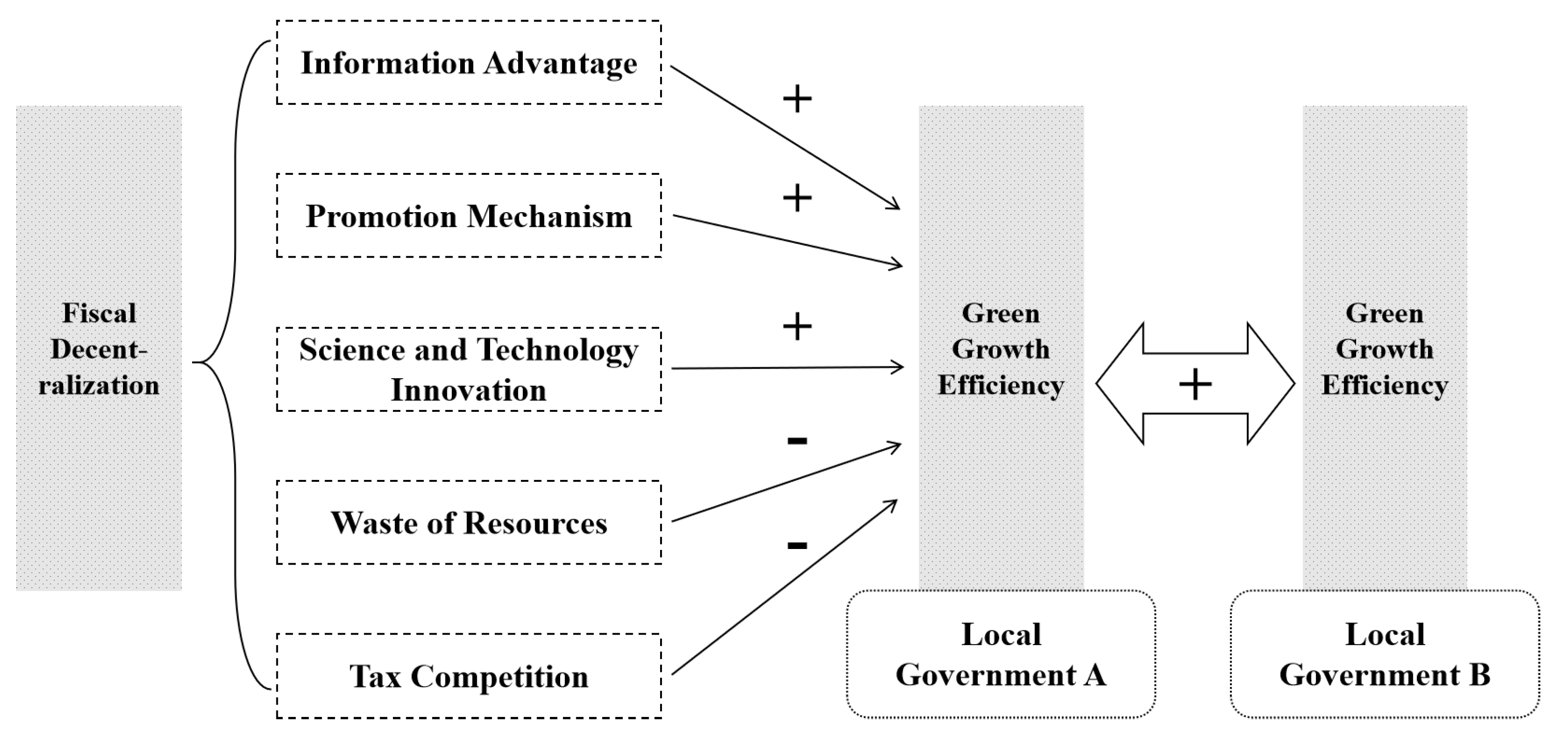
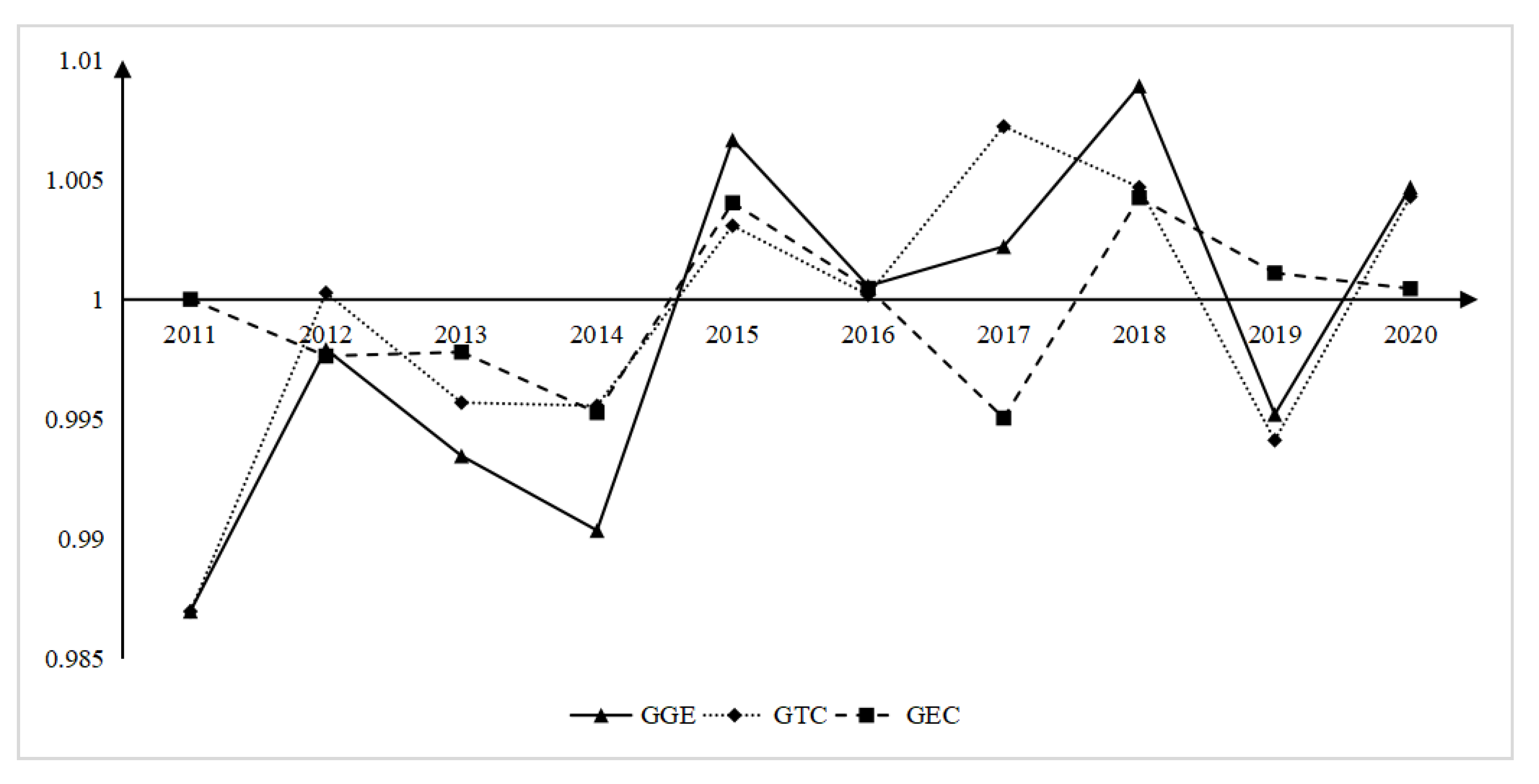
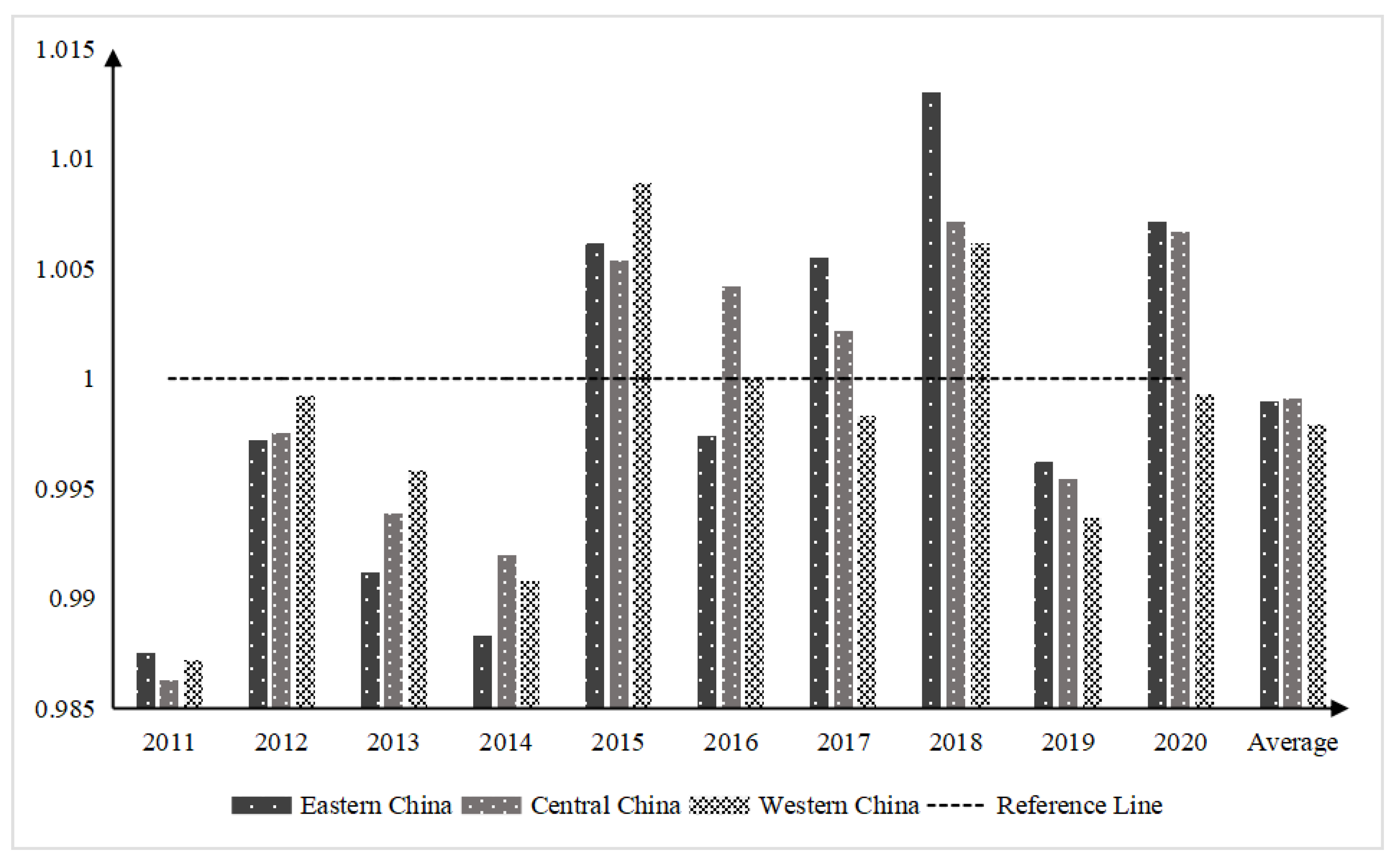
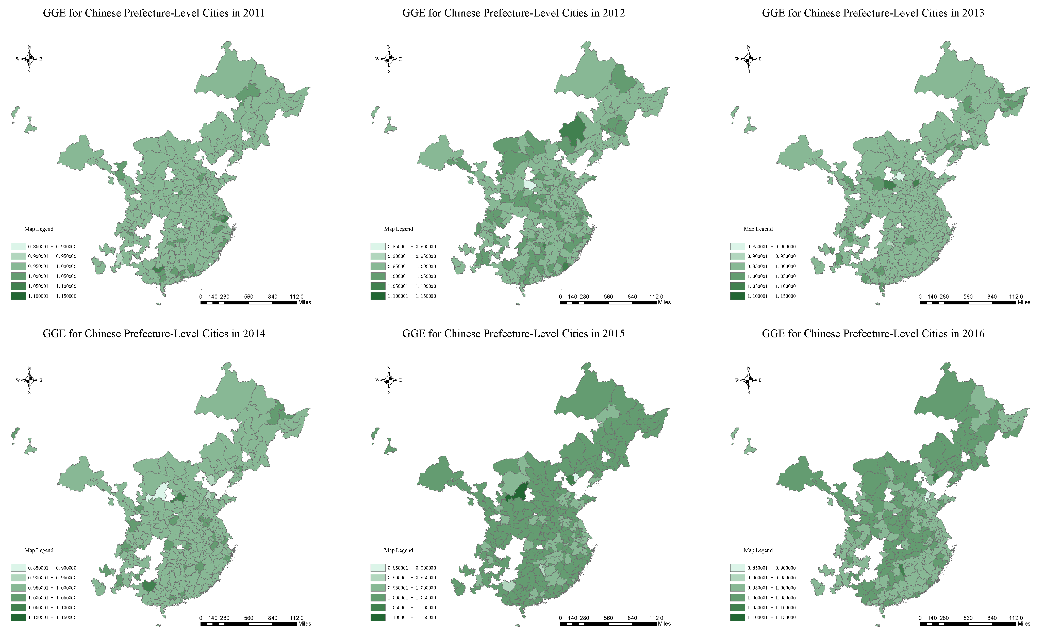
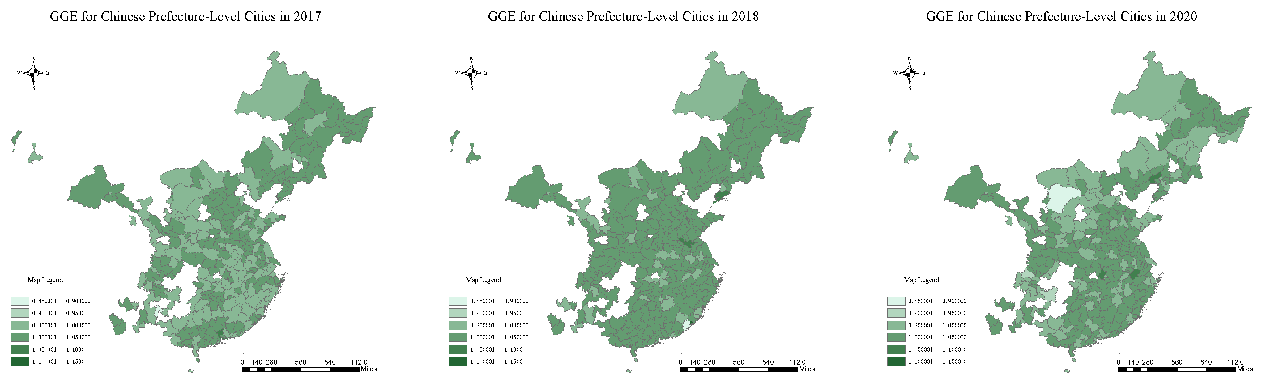
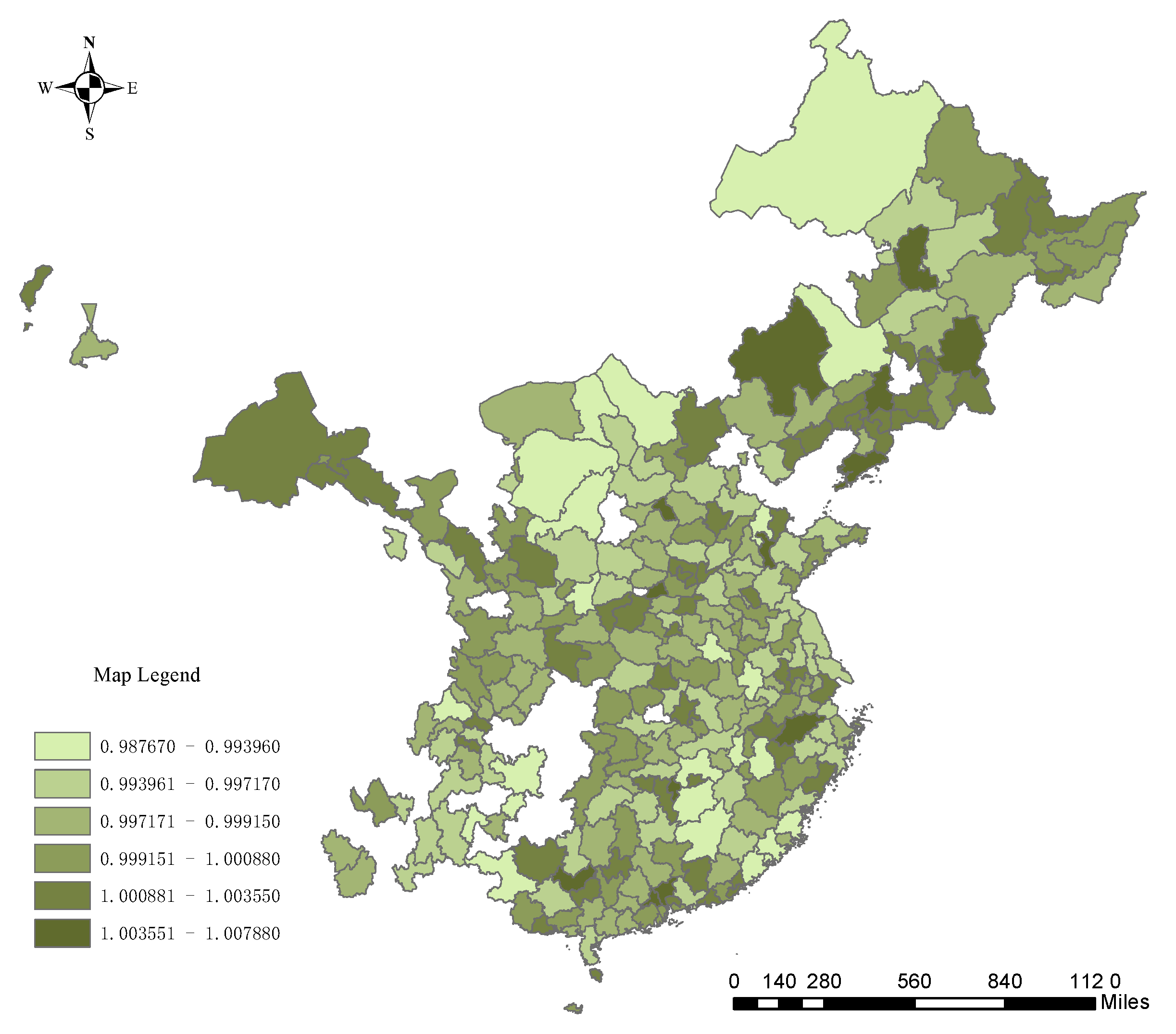
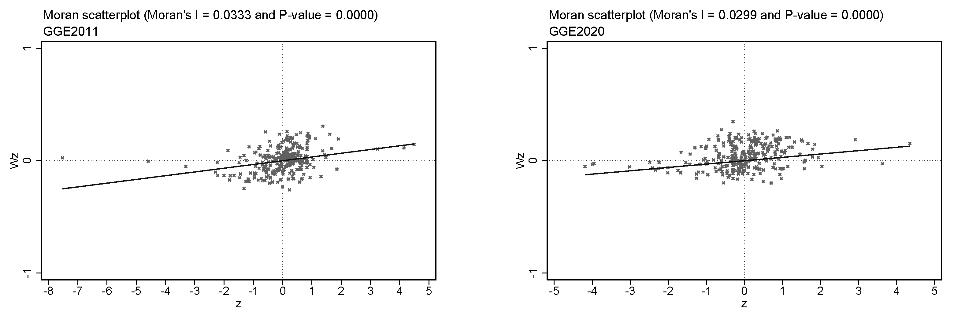
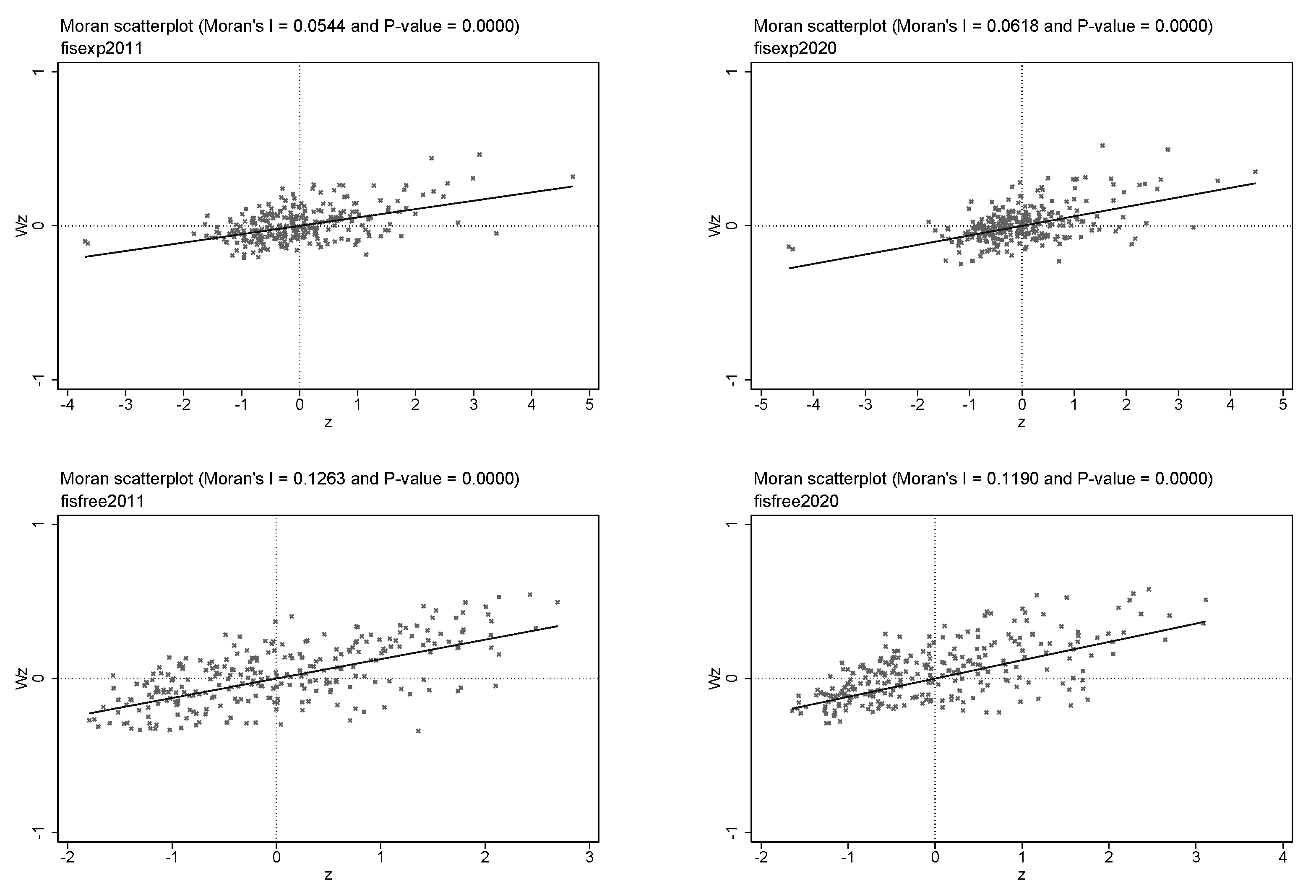
Table 1.
Input–output indicators in the SBM-DDF model.
| Variables | Calculation Method | Unit of Measure | |
|---|---|---|---|
| Input Indicator | Capital input | Fixed capital stock under the perpetual inventory method | Million CNY |
| Labor input | Number of employees in workplaces at the end of the year | Million | |
| Energy input | Total electricity consumption of the whole society | Billion kWh | |
| Expected Output Indicator | Economic output | GDP with 2010 as base period | Million CNY |
| Unexpected Output Indicator | Wastewater emissions | Industrial wastewater emissions | Million tons |
| Sulfur dioxide emissions | Industrial sulfur dioxide emissions | Tons | |
| Smoke and dust emissions | Industrial smoke and dust emissions | Tons | |
| Carbon emissions | Total carbon emissions from three scopes | Million tons | |
Data Source: China Statistical Yearbook, China City Statistical Yearbook, China Fixed Asset Investment Yearbook, China Energy Statistical Yearbook, China Industrial Statistical Yearbook, China Agricultural Statistical Yearbook and China Animal Husbandry Yearbook.
Table 2.
Variables in dynamic panel regression model.
| Variables | Meaning of Variable | Calculation Method | |
|---|---|---|---|
| Dependent Variable | GGE | Green growth efficiency | Green growth efficiency of each prefecture-level city calculated according to SBM-DDF model |
| Core Explanatory Variables | fisexp | Decentralization of fiscal expenditures | Fiscal expenditure per capita at the prefecture level divided by the sum of fiscal expenditure per capita at the prefecture, provincial and national levels |
| fisfree | Decentralization of fiscal freedom | Fiscal revenues divided by fiscal expenditures at the prefecture level | |
| Control Variables | ind | Industrial structure | Share of secondary and tertiary output in GDP |
| open | Degree of openness to foreign countries | Foreign capital actually used in the year being converted into CNY at the exchange rate of the year and divided by GDP | |
| eco | Economic development | Real GDP divided by total population and logarithmized | |
| tec | Scientific and technological development | Patents granted in the year per ten million people | |
| edu | Level of education | Number of students enrolled in secondary and elementary school | |
| imp | Import dependence | Total imports for the year divided by GDP | |
| exp | Export dependence | Total exports for the year divided by GDP | |
Data Source: China City Statistical Yearbook and China Customs Statistics Database.
Table 3.
Descriptive statistics of variables.
| Variables | Obs | Mean | Std. Dev. | Min | Max | p1 | p99 |
|---|---|---|---|---|---|---|---|
| GGE | 2710 | 0.999 | 0.015 | 0.870 | 1.124 | 0.957 | 1.041 |
| 2710 | 0.403 | 0.099 | 0.001 | 0.892 | 0.222 | 0.718 | |
| 2710 | 0.456 | 0.221 | 0.057 | 1.541 | 0.099 | 1.007 | |
| 2710 | 0.877 | 0.077 | 0.501 | 1 | 0.618 | 0.994 | |
| 2710 | 0.016 | 0.017 | 0 | 0.199 | 0 | 0.069 | |
| 2710 | 4.473 | 0.286 | 3.751 | 5.593 | 3.906 | 5.249 | |
| 2710 | 0.014 | 0.057 | 0 | 1.579 | 0 | 0.151 | |
| 2710 | 0.053 | 0.036 | 0.003 | 0.231 | 0.005 | 0.164 | |
| 2710 | 0.071 | 0.180 | 0 | 4.588 | 0 | 0.714 | |
| 2710 | 0.104 | 0.168 | 0 | 1.711 | 0.001 | 0.954 |
Table 4.
Static and dynamic panel regression results.
| Variables | GGE | |||
|---|---|---|---|---|
| (1) | (2) | (3) | (4) | |
| — | −0.218 *** (−9.19) | — | −0.235 *** (−9.68) | |
| fisexp | 0.062 *** (3.99) | 0.047 *** (2.68) | — | — |
| fisfree | — | — | −0.039 *** (−7.07) | −0.042 *** (−7.21) |
| ind | 0.128 *** | 0.114 *** | 0.096 *** | 0.079 *** |
| (7.54) | (5.80) | (5.64) | (4.14) | |
| open | −0.062 * | −0.078 ** | −0.020 | −0.040 |
| (−1.65) | (−2.04) | (−0.60) | (−1.10) | |
| eco | −0.037 *** | −0.041 *** | −0.012 * | −0.017 ** |
| (−5.99) | (−6.08) | (−1.89) | (−2.56) | |
| tec | 0.018 | 0.006 | 0.010 | −0.002 |
| (0.81) | (0.33) | (0.61) | (−0.14) | |
| edu | 0.081 | 0.265 *** | 0.003 | 0.156 ** |
| (1.58) | (4.02) | (0.06) | (2.25) | |
| imp | −0.001 | −0.000 | −0.001 | −0.001 |
| (−1.13) | (−0.36) | (−1.29) | (−0.61) | |
| exp | −0.002 | −0.003 | 0.001 | 0.001 |
| (−0.52) | (−0.62) | (0.25) | (0.12) | |
| Constant | 1.022 *** | 1.270 *** | 0.984 *** | 1.254 *** |
| (37.65) | (29.14) | (38.27) | (29.18) | |
| Fixed effect | Yes | Yes | Yes | Yes |
| N | 2710 | 2439 | 2710 | 2439 |
| 0.035 | 0.076 | 0.051 | 0.100 | |
| 12.242 | 17.627 | 18.203 | 21.074 | |
Note: 1. t statistics in parentheses, which also applies to the following tables. 2. ***, ** and * indicate that the coefficients are significant at the 1%, 5%, and 10% significance levels, respectively. 3. Fixed effects are individual fixed effects. Standard errors are city clustering standard errors.
Table 5.
Global Moran’s I of , and for 2011–2020 (with ).
| GGE | fisexp | fisfree | ||||
|---|---|---|---|---|---|---|
| Moran’s I | p-Value | Moran’s I | p-Value | Moran’s I | p-Value | |
| 2011 | 0.033 | 0.000 | 0.054 | 0.000 | 0.126 | 0.000 |
| 2012 | −0.003 | 0.875 | 0.056 | 0.000 | 0.125 | 0.000 |
| 2013 | 0.012 | 0.003 | 0.054 | 0.000 | 0.116 | 0.000 |
| 2014 | 0.009 | 0.014 | 0.056 | 0.000 | 0.121 | 0.000 |
| 2015 | 0.018 | 0.000 | 0.054 | 0.000 | 0.117 | 0.000 |
| 2016 | 0.047 | 0.000 | 0.054 | 0.000 | 0.120 | 0.000 |
| 2017 | 0.020 | 0.000 | 0.055 | 0.000 | 0.116 | 0.000 |
| 2018 | 0.002 | 0.290 | 0.057 | 0.000 | 0.122 | 0.000 |
| 2019 | 0.009 | 0.012 | 0.058 | 0.000 | 0.116 | 0.000 |
| 2020 | 0.030 | 0.000 | 0.062 | 0.000 | 0.119 | 0.000 |
Table 6.
Tests for spatial econometric model choice.
| Tests for Spatial Econometric Model Choice | |||||
|---|---|---|---|---|---|
| LM test | no error | 1.251 | 1.021 | 1.124 | 6.011 |
| (0.14) | (0.16) | (0.15) | (0.05) | ||
| no error (robust) | 5.242 | 4.353 | 4.918 | 30.282 | |
| (0.05) | (0.07) | (0.06) | (0.00) | ||
| no lag | 198.773 | 422.571 | 482.820 | 263.362 | |
| (0.00) | (0.00) | (0.00) | (0.00) | ||
| no lag (robust) | 206.665 | 528.370 | 272.462 | 163.372 | |
| (0.00) | (0.00) | (0.00) | (0.00) | ||
| Hausman test | Fixed | Fixed | Fixed | Fixed | |
| LR test | Individual Fixed | Individual Fixed | Individual Fixed | Individual Fixed | |
Table 7.
Dynamic SAR model results.
| Variables | fisexp | fisfree | ||||||
|---|---|---|---|---|---|---|---|---|
(5) | (6) | (7) | (8) | (9) | (10) | (11) | (12) | |
| −0.163 *** | −0.147 *** | −0.156 *** | −0.157 *** | −0.172 *** | −0.155 *** | −0.158 *** | −0.164 *** | |
| (−8.33) | (−7.42) | (−7.92) | (−7.95) | (−8.83) | (−7.90) | (−8.01) | (−8.34) | |
| 0.324 *** | 0.362 *** | 0.865 *** | 0.402 *** | 0.302 *** | 0.333 *** | 0.846 *** | 0.373 *** | |
| (13.92) | (12.37) | (27.53) | (14.10) | (12.78) | (11.14) | (24.69) | (12.76) | |
| 0.123 *** | 0.084 ** | 0.149 *** | 0.117 *** | 0.103 *** | 0.051 | 0.127 *** | 0.088 ** | |
| (4.07) | (2.25) | (3.31) | (3.16) | (3.40) | (1.36) | (2.78) | (2.36) | |
| fisexp | 0.030 ** | 0.033 ** | 0.016 | 0.030 ** | — | — | — | — |
| (2.07) | (2.27) | (1.13) | (2.10) | |||||
| fisfree | — | — | — | — | −0.028 *** | −0.030 *** | −0.012 *** | −0.027 *** |
| (−5.95) | (−6.23) | (−2.62) | (−5.62) | |||||
| ind | 0.059 *** | 0.067 *** | 0.009 | 0.056 *** | 0.040 ** | 0.048 *** | 0.002 | 0.039 ** |
| (3.33) | (3.68) | (0.50) | (3.11) | (2.27) | (2.65) | (0.14) | (2.20) | |
| open | −0.048 | −0.052 * | −0.019 | −0.049 | −0.024 | −0.027 | −0.010 | −0.027 |
| (−1.59) | (−1.70) | (−0.67) | (−1.62) | (−0.80) | (−0.90) | (−0.34) | (−0.88) | |
| eco | −0.024 *** | −0.025 *** | −0.012 ** | −0.022 *** | −0.010 | −0.010 | −0.005 | −0.008 |
| (−4.10) | (−4.24) | (−2.02) | (−3.75) | (−1.60) | (−1.61) | (−0.93) | (−1.42) | |
| tec | 0.004 | 0.003 | −0.004 | 0.003 | −0.002 | −0.002 | −0.006 | −0.002 |
| (0.31) | (0.24) | (−0.38) | (0.27) | (−0.14) | (−0.21) | (−0.55) | (−0.14) | |
| edu | 0.183 *** | 0.192 *** | 0.110 ** | 0.171 *** | 0.116 ** | 0.123 ** | 0.084 | 0.110 ** |
| (3.49) | (3.63) | (2.19) | (3.26) | (2.17) | (2.28) | (1.63) | (2.06) | |
| imp | −0.000 | −0.000 | 0.000 | −0.000 | −0.000 | −0.000 | −0.000 | −0.001 |
| (−0.12) | (−0.13) | (0.00) | (−0.17) | (−0.21) | (−0.22) | (−0.03) | (−0.25) | |
| exp | −0.000 | 0.001 | 0.003 | 0.001 | 0.002 | 0.003 | 0.004 | 0.003 |
| (−0.03) | (0.23) | (0.56) | (0.22) | (0.34) | (0.56) | (0.71) | (0.54) | |
| N | 2439 | 2439 | 2439 | 2439 | 2439 | 2439 | 2439 | 2439 |
| Log(L) | 7060.654 | 7040.261 | 7182.696 | 7061.247 | 7078.246 | 7058.911 | 7185.902 | 7076.528 |
Note: ***, ** and * indicate that the coefficients are significant at the 1%, 5%, and 10% significance levels.
Table 8.
Effect decomposition of main variables (with ).
| Effect | (8) | (12) | ||||
|---|---|---|---|---|---|---|
| fisexp | ind | edu | fisfree | ind | edu | |
| Direct effect in short term | 0.033 ** | 0.058 *** | 0.174 *** | −0.027 *** | 0.041 ** | 0.112 ** |
| Indirect effect in short term | 0.021 ** | 0.036 *** | 0.109 *** | −0.015 *** | 0.023 ** | 0.063 ** |
| Total effect in short term | 0.054 ** | 0.094 *** | 0.283 *** | −0.043 *** | 0.063 ** | 0.176 ** |
| Direct effect in long term | 0.029 ** | 0.050 *** | 0.151 *** | −0.024 *** | 0.035 ** | 0.097 ** |
| Indirect effect in long term | 0.022 ** | 0.038 *** | 0.114 *** | −0.014 *** | 0.021 ** | 0.060 ** |
| Total effect in long term | 0.050 ** | 0.088 *** | 0.266 *** | −0.038 *** | 0.056 ** | 0.157 ** |
Note: ***, ** indicate that the coefficients are significant at the 1%, 5% significance levels.
Table 9.
Dynamic SAR model results for different time periods (with ).
| Variables | 2011–2014 | 2015–2020 | ||||||
|---|---|---|---|---|---|---|---|---|
(13) | (14) | (15) | (16) | (17) | (18) | (19) | (20) | |
| −0.269 *** | −0.252 *** | −0.258 *** | −0.256 *** | −0.111 *** | −0.096 *** | −0.078 *** | −0.099 *** | |
| (−9.07) | (−8.59) | (−8.55) | (−8.70) | (−4.23) | (−3.60) | (−2.93) | (−3.72) | |
| 0.090 * | 0.193 *** | 0.715 *** | 0.197 *** | 0.300 *** | 0.220 *** | 0.891 *** | 0.296 *** | |
| (1.81) | (2.96) | (6.58) | (3.10) | (9.42) | (5.00) | (18.44) | (6.86) | |
| 0.073 | 0.005 | 0.211 ** | 0.039 | −0.012 | −0.131 ** | 0.163 ** | −0.060 | |
| (1.45) | (0.08) | (2.18) | (0.58) | (−0.29) | (−2.33) | (1.98) | (−1.06) | |
| fisexp | 0.037 | 0.044 | 0.052 * | 0.042 | 0.057 ** | 0.061 ** | 0.069 ** | 0.059 ** |
| (1.31) | (1.53) | (1.83) | (1.45) | (2.04) | (2.11) | (2.49) | (2.06) | |
| Control Variables | Yes | Yes | Yes | Yes | Yes | Yes | Yes | Yes |
| N | 813 | 813 | 813 | 813 | 1626 | 1626 | 1626 | 1626 |
| Log(L) | 2605.098 | 2605.698 | 2617.375 | 2606.208 | 4001.623 | 3975.637 | 4033.971 | 3983.749 |
Note: ***, ** and * indicate that the coefficients are significant at the 1%, 5%, and 10% significance levels.
Table 10.
Dynamic SAR model results for different time periods (with ).
| Variables | 2011–2014 | 2015–2020 | ||||||
|---|---|---|---|---|---|---|---|---|
(21) | (22) | (23) | (24) | (25) | (26) | (27) | (28) | |
| −0.265 *** | −0.247 *** | −0.254 *** | −0.252 *** | −0.113 *** | −0.099 *** | −0.084 *** | −0.102 *** | |
| (−8.95) | (−8.44) | (−8.42) | (−8.57) | (−4.32) | (−3.72) | (−3.13) | (−3.84) | |
| 0.082 | 0.178 *** | 0.683 *** | 0.183 *** | 0.299 *** | 0.222 *** | 0.902 *** | 0.297 *** | |
| (1.63) | (2.72) | (5.96) | (2.86) | (9.41) | (5.05) | (18.87) | (6.88) | |
| 0.079 | 0.013 | 0.214 ** | 0.049 | −0.009 | −0.118 ** | 0.204 ** | −0.049 | |
| (1.58) | (0.18) | (2.19) | (0.72) | (−0.20) | (−2.07) | (2.45) | (−0.86) | |
| fisfree | −0.022 ** | −0.020 ** | −0.016 | −0.020 * | −0.009 | −0.008 | −0.013 | −0.008 |
| (−2.21) | (−1.98) | (−1.60) | (−1.94) | (−1.05) | (−0.89) | (−1.46) | (−0.87) | |
| Control Variables | Yes | Yes | Yes | Yes | Yes | Yes | Yes | Yes |
| N | 813 | 813 | 813 | 813 | 1626 | 1626 | 1626 | 1626 |
| Log(L) | 2605.882 | 2605.669 | 2616.349 | 2606.293 | 4000.570 | 3974.415 | 4032.748 | 3982.580 |
Note: ***, ** and * indicate that the coefficients are significant at the 1%, 5%, and 10% significance levels.
Table 11.
Dynamic SAR model results for Eastern, Central, and Western China (with ).
| Variables | fisexp | fisfree | ||||
|---|---|---|---|---|---|---|
| Eastern (29) | Central (30) | Western (31) | Eastern (32) | Central (33) | Western (34) | |
| −0.149 *** | −0.237 *** | −0.149 *** | −0.155 *** | −0.245 *** | −0.156 *** | |
| (−4.60) | (−7.11) | (−4.08) | (−4.80) | (−7.37) | (−4.26) | |
| 0.398 *** | 0.396 *** | 0.307 *** | 0.366 *** | 0.383 *** | 0.305 *** | |
| (9.40) | (8.70) | (5.39) | (8.35) | (8.36) | (5.34) | |
| 0.123 ** | 0.222 *** | 0.018 | 0.087 | 0.218 *** | 0.015 | |
| (2.15) | (3.86) | (0.25) | (1.51) | (3.80) | (0.22) | |
| fisexp | 0.044 *** (3.47) | 0.028 *** (4.39) | 0.029 ** (2.08) | — | — | — |
| fisfree | — | — | — | −0.032 *** (−3.51) | −0.020 *** (−3.15) | −0.021 * (−1.82) |
| Control Variables | Yes | Yes | Yes | Yes | Yes | Yes |
| N | 855 | 882 | 702 | 855 | 882 | 702 |
| Log(L) | 2434.412 | 2659.121 | 2022.276 | 2440.040 | 2663.664 | 2023.765 |
Note: ***, ** and * indicate that the coefficients are significant at the 1%, 5%, and 10% significance levels.
Disclaimer/Publisher’s Note: The statements, opinions and data contained in all publications are solely those of the individual author(s) and contributor(s) and not of MDPI and/or the editor(s). MDPI and/or the editor(s) disclaim responsibility for any injury to people or property resulting from any ideas, methods, instructions or products referred to in the content. |
© 2024 by the authors. Licensee MDPI, Basel, Switzerland. This article is an open access article distributed under the terms and conditions of the Creative Commons Attribution (CC BY) license (https://creativecommons.org/licenses/by/4.0/).
Share and Cite
MDPI and ACS Style
Li, Y.; Bai, L. Analyzing Green Growth Efficiency in China and Investigating the Spatial Effects of Fiscal Decentralization: Case Study of Prefecture-Level Cities. Sustainability 2024, 16, 3408. https://doi.org/10.3390/su16083408
AMA Style
Li Y, Bai L. Analyzing Green Growth Efficiency in China and Investigating the Spatial Effects of Fiscal Decentralization: Case Study of Prefecture-Level Cities. Sustainability. 2024; 16(8):3408. https://doi.org/10.3390/su16083408
Chicago/Turabian StyleLi, Yiming, and Liru Bai. 2024. "Analyzing Green Growth Efficiency in China and Investigating the Spatial Effects of Fiscal Decentralization: Case Study of Prefecture-Level Cities" Sustainability 16, no. 8: 3408. https://doi.org/10.3390/su16083408
Note that from the first issue of 2016, this journal uses article numbers instead of page numbers. See further details here.