Sustainable Development Strategies in Power Systems: Day-Ahead Stochastic Scheduling with Multi-Sources and Customer Directrix Load Demand Response

Abstract

Increasing the installed capacity of renewable energy sources (RESs) in the power system is significant for advancing sustainable development. As the proportion of RESs rapidly increases in power systems, the inherent stochasticity and variability of renewable energies significantly reduce the regulatory capacity of generation resources. To compensate for the lack of power system flexibility, it is necessary to coordinate the participation of load-side resources in demand response (DR). Therefore, this paper proposes a solution to the diminished flexibility of power systems. It introduces a day-ahead stochastic scheduling model for an integrated thermal-hydro-wind-solar system. This model relies on customer directrix load (CDL) to efficiently absorb RES output. CDL represents an ideal load profile shape. Firstly, the stochastic scenario sets of RES output were modeled using Monte Carlo simulations, and the complementary characteristics between wind and solar output are considered using Copula theory. Then, CDL is introduced into day-ahead scheduling model, which considers relevant demand-side responsive load constraints. Secondly, customer-side DR effectiveness model is proposed to obtain the shaping load profile after DR, based on quantitative customer response effectiveness evaluation metrics. Lastly, system-side stochastic scheduling model of high-proportion RES power system is proposed based on the shaping load profile. Case studies were conducted on a modified IEEE-6 bus system. These studies show that the model effectively addresses the uncertainty of RES. It improves the power system’s regulation capability. Additionally, it promotes the absorption of RES.

1. Introduction

With escalating energy demand and advancements in the energy sector, carbon dioxide emissions have surged annually. It is crucial to advance decarbonization in power generation, develop renewable energy source (RESs) technologies, foster the transition towards RESs, and build a new power system predominantly reliant on RESs for achieving China’s carbon peaking and carbon neutrality goals [1].

The conventional power system depends on substantial capacity of thermal units and the secure, stable operation of backup system for wind and solar power. However, renewable resources like wind and solar power are highly susceptible to climatic, seasonal, and temperature variations, introducing significant uncertainty and volatility. As the integration of these resources into the grid increases, the system faces amplified uncertainty at both the generation and consumption ends, complicating operation and challenging its security, stability, and dynamic balance [2]. Thus, it is of paramount importance to study the optimal scheduling of systems with a high proportion of RESs. Demand response (DR) can effectively integrate flexible loads, reducing the use of high-cost thermal units [3]; thereby, reducing the load in peak periods can avoid unit capacity expansions and ease bottlenecks in the power system [4]. DR strategies based on demand-side resource management have emerged as crucial for ensuring reliable power supply and the safe and stable operation of new power systems due to their flexible regulation, high potential for adjustment, minimal grid impact, and low costs [5]. In the current study, researchers generally categorize DR into price-based DR (PDR) and incentive-based DR (IDR) [6,7]. PDR guides electricity consumers to optimize their own load profiles through the setting of price mechanisms like time-of-use (TOU) tariffs and categorized electricity price. IDR includes modes of operation such as interruptible load, incentive coupon issuance, and direct load control, which do not involve tariffs and customers will not bear direct benefit losses [8]. In Ref. [9], a solid estimation of consumer demand and its relationship with TOU tariffs is offered. Ref. [10] proposes a dynamic tariff scheme based on linear regression, which guides residential customers to participate in DR and addresses the optimization challenge of DR using a particle swarm optimization algorithm. Ref. [11] introduces an incentive-based DR (IDR) strategy, employing two-stage optimization approach to minimize the cost of flexibility management and improve the peak-to-average ratio of the community microgrid load profile. Ref. [12] explores an optimization problem for operating energy hubs (EHs), aiming to enhance customer benefit and reduce the overall operational cost of the EH system, in the context of both PDR and IDR programs. However, the two DR mechanisms mentioned above currently suffer from the following shortcomings: PDR is an involuntary regulation method and is affected by differences in customers’ perceptions of the DR benefits, which is not customer-friendly, and its large-scale rollout can lead to the over-regulation or rebound of loads [13,14]. IDR widely adopts customer baseline load (CBL) to evaluate customer contributions, but in large-scale DR, the calculation of CBL for large number of customers faces enormous data calculation, storage and communication pressure, and the accuracy and authenticity of CBL cannot be guaranteed [15].

For these reasons, some scholars proposed the strategy of customer directrix load (CDL), a desired load profile that offsets power system fluctuations effectively [16,17]. Customers can make their load profiles as close as possible to the CDL in order to reap the benefits. CDL-based DR is simple and easy to implement, has the characteristics of widespread promotion and normalized implementation, and can well support the construction of new power systems, so it has received extensive attention from scholars. Ref. [18] proposes a calculation model of nodal customer directrix load (NCDL) with robust security, which can guarantee that the power flow across all lines remains within established limits for any real response outcomes within the designated DR range. The above literature takes the associated network constraints and the uncertainty of flexible loads into account, however has not yet considered the uncertainty of RES output, which is also a factor that should not be ignored in scheduling optimization. The scenario optimization method is one of the main approaches to study the uncertainty of RES, and uncertainty is considered by generating sets of scenarios through Monte Carlo simulation. This method can accurately characterize the random variables. While the current CDL-based DR optimal scheduling model does not consider hydro units, the modeling of joint optimal scheduling problems of cascade hydropower plants has emerged as a challenging and significant problem in the field of optimal scheduling. Ref. [19] introduces a scheduling strategy for a thermal-hydro-wind-solar system that incorporates the impacts of water head and discharges within a single function. This strategy enables the transformation of the head-dependent hydropower conversion function into a piecewise linear function, which can be efficiently solved using a mixed-integer programming (MIP) model.

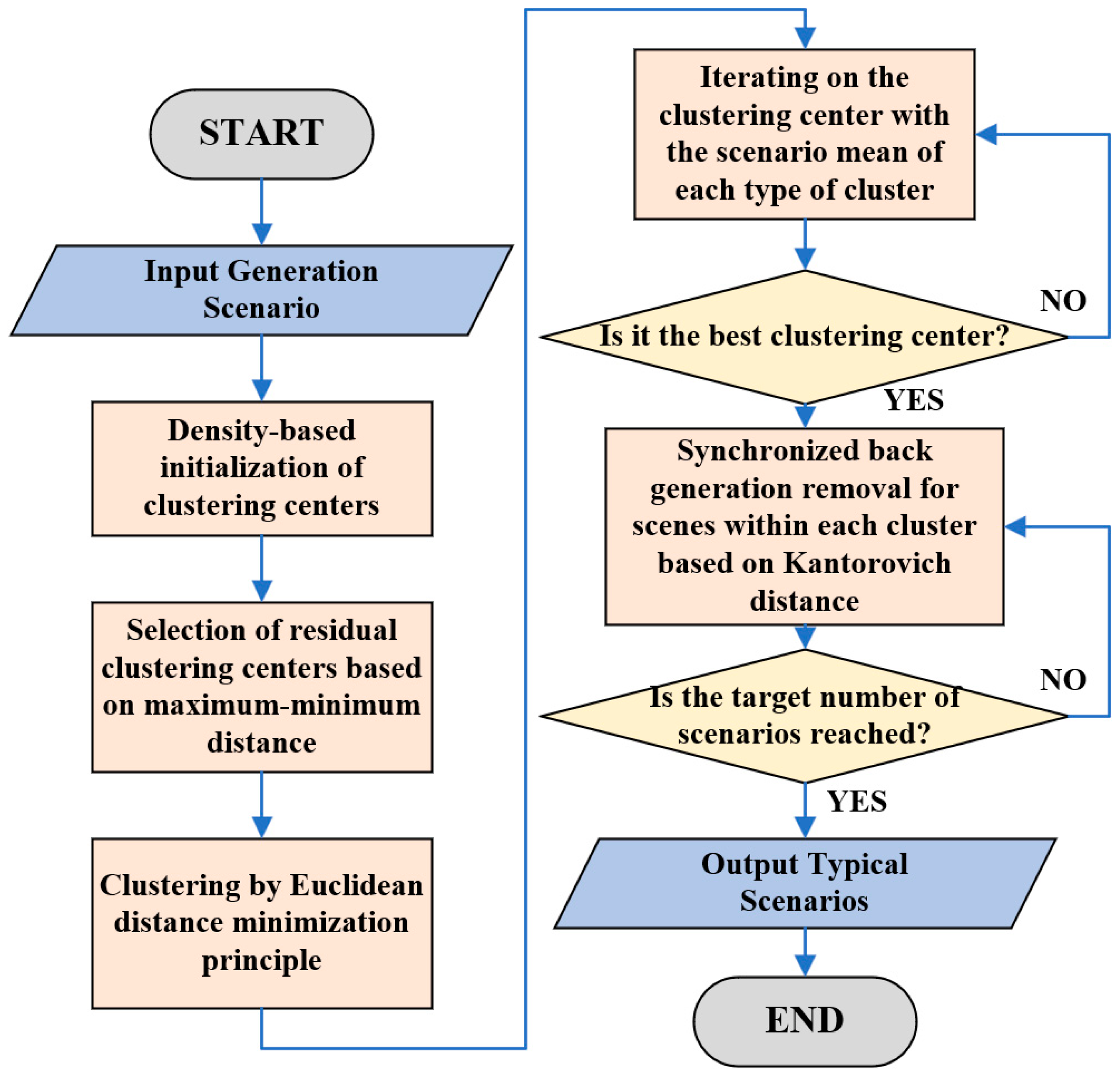
To address the above challenges, we propose a multi-sources stochastic coordinated scheduling model based on CDL-based DR. Compared with traditional methods, the model we propose integrates the uncertainty of RES through various scenarios generated using Monte Carlo simulation. By examining the complementary traits between wind and solar generation, we can establish the fundamental functions of both. The scenarios can be generated by using the Copula function, which is used to describe the complementary traits of wind and solar output. A fast scenario reduction technique based on improved k-means clustering and the SBR algorithm [20] is employed to balance precision with computational efficiency. The dynamic characteristics of hydro units, which are not currently considered, are also included to improve energy efficiency and stable supply and reduce energy volatility through multi-energy complementarity. Finally, case simulations were carried out by means of a modified IEEE 6-bus power system arithmetic example, and the results of the case study indicate that the proposed model can effectively improve system flexibility, reduce the curtailment of RES in a high-proportion RES power system, and obtain the intermediate scheduling solutions in the base case with the uncertainty of RESs.

The main contributions are presented as follows:

(1)

Compared with traditional stochastic optimization methods where the objective function is to minimize the cost of system operation in all scenarios, the proposed model aims to obtain a dispatch solution with a stable operating cost in the base case. This dispatch solution allows for the power system to operate under the forecasted base case and can safely redispatch all units in response to real-time fluctuations in RES output.

(2)

We introduce the dynamic characteristics of cascade hydro units and CDL-based DR in day-ahead stochastic scheduling model with RES uncertainty for the first time. The complementary characteristics of wind and solar are considered and modeled using the t-Copula function. These all aim to improve energy efficiency, ensure stable supply, and reduce energy fluctuations through multi-sources complementary and coordinated scheduling.

We concisely encapsulate this paper’s structure: after this introduction, Section 2 introduces the concept of CDL, defines the response effect metrics and incentives for CDL. Section 3 introduces our methodology, focusing on the novel day-ahead stochastic scheduling model incorporating CDL-based DR. In Section 4, we detail the formulation of our model, elucidating on the use of Copula theory and Monte Carlo simulations for addressing uncertainties in RESs. Section 5 applies the proposed model to a modified IEEE-6 bus system, showcasing the practical application and effectiveness of our approach through case studies. The discussion in Section 6 extends the analysis of our findings, contemplating their broader implications and suggesting avenues for future research. Section 7 synthesizes our contributions, emphasizing the effectiveness of our novel stochastic scheduling method in enhancing RES consumption and robustness of system operation.

2. Customer Directrix Load

In this section, we will introduce the concept of CDL and define the response effect metrics and incentives for CDL.

2.1. CDL-Based DR Strategy

In the domain of power systems, uncontrollable devices such as RES and inflexible loads are the sources of power fluctuations. To uphold the stability of power systems, controllable resources including conventional power sources, DR, and curtailment of RES are required to counteract these fluctuations and ensure real-time power balance. Ref. [16] posits that, based on the regulation needs generated by RES and inflexible loads within the system, the ideal shape of the flexible load profile was computed and termed CDL. CDL serves both as a target for consumer adjustments and as a benchmark for evaluating the contributions of consumers to system balance.

In this study, the electric load was divided into flexible loads that participate in DR and inflexible loads that do not participate in the DR as Equation (1). All customers on the demand side who are interested in participating in the DR as an adjustable resource were registered. Since load collimation is only concerned with the shape of the load profile, industrial, commercial, and residential customers could participate directly.

$$P_{dt}=P_{DR,t}+P_{nDR,t}$$

(1)

where $P_{DR,t}$ is flexible loads at $t$ time; $P_{nDR,t}$ is inflexible loads at $t$ time; $P_{dt}$ is the electric load demand of load at $t$ time.

The DR center calculates the CDL based on the network-wide operating data before the day and releases the load parity to the whole community. Customers participating in the DR make decisions about their electricity usage for the following day, based on the load baseline and their personal energy needs. They aim to align their load profile as closely as possible with the CDL to maximize their incentive compensation. This strategy encourages users to modify their consumption patterns to better match the available supply, contributing to the overall efficiency and stability of the power system.

It is noted the power system operates at its optimal state when the shape of the adjustable load exactly matches the CDL, preventing the need for conventional power adjustments and the curtailment of RESs. In such a scenario, the optimal solution for flexible loads is identified through optimization models as the value of CDL. However, due to the physical and comfort limitations of customers, the actual reshaped load profile may only approximate, not coincide with, the desired load profile. Consequently, per standard power dispatch models, conventional power resources and reduction in RES outputs are utilized to mitigate fluctuations and achieve power balance.

We employed the L-1 norm for normalizing the load profile, indicating that alternative normalization methods do not affect the applicability of CDL. The per unit load profile eliminates the features in the order of magnitude and retains only the features in the shape of the load profile, which can provide a load shaping target for all DR participants as follows:

$$P_{DR,t}^{*}=\frac{P_{DR,t}}{C_D},t=1,2,\dots ,T$$

(2)

$$C_D={\displaystyle \sum _{t=1}^T{P}_{DR,t}}$$

(3)

where $T$ is the total number of hours in the dispatch; $C_D$ is the total electrical consumption of the flexible load at $t$ time, also known as the total flexible electricity; $P_{DR,t}^{*}$ is the per unit of flexible load.

The purpose of the CDL-based DR is to encourage customers to modify the shape of their load profile, achieving peak shaving and valley filling without changing the total electricity consumption thereby ensuring energy efficiency for consumers. Hence, the following constraints need to be considered:

$$\left\{\begin{array}{c}{\displaystyle \sum _{t=1}^T}{P}_{\mathrm{DR},t}^{\ast }=1\\ 0⩽P_{\mathrm{DR},t}^{\ast }⩽1\end{array}\right.$$

(4)

In addition, it is necessary to consider the system load balance constraints, thermal unit constraints, RES capacity constraints and power flow constraints, etc. The calculation model of CDL and its objective function and associated constraints will be detailed in Section 3.

2.2. Response Evaluation and Incentives

The DR center needs to measure the effectiveness of customer response and set up a reasonable incentive subsidy mechanism to ensure that customers are proactive and obtain positive feedback in the DR process. Therefore, a metric is defined to measure the similarity between the customer’s actual load profile and the load CDL, also known as the CDL similarity:

$$\left\{\begin{array}{c}E=E\left(l_t^{\ast },P_{\mathrm{DR},t}^{\ast }\right)={\mathrm{e}}^{-\epsilon d^2}\\ d=\sqrt{{\displaystyle \sum _{t=1}^T}{(l_t^{\ast }-P_{\mathrm{DR},t}^{\ast })}^2}\end{array}\right.$$

(5)

where $d$ is the Euclidean distance between the two profiles, and $d$ is converted to a similarity metric $E$ between the intervals (0,1] by the constant value $\epsilon$. Since $d$ is calculated using the per unit value of the load profiles, the value of $d$ is approximately between 0 and 1. When both load profiles are exactly same, the value of $d$ is 0. Figure 1 visualizes the sensitivity of the $E$ to $\epsilon$. It is observed that when $\epsilon$ is set to 5, it is better converts $d$ to the similarity metric $E$. Therefore, we set $\epsilon$ to 5 in the simulations.

It is commonly assumed in the current stage of research that customers participating in DR are completely rational, which means that customers will combine subsidy incentives to minimize the amount of change in their own electricity use under the premise of ensuring that the total amount of electricity used does not change and similarity of alignment before and after participation in DR improves $\Delta E$. It is out of the scope of this paper to discuss the non-rationality of consumers. Future work may address the impact of non-rational behavior. The model is as follows:

$$\left\{\begin{array}{l}\min {\displaystyle \sum _{t=1}^T}{(P_{l,\mathrm{DR},t}^{\ast }-P_{l,t}^{\ast })}^2\\ \mathrm{s}.\mathrm{t}. E\left(P_{l,\mathrm{DR},t}^{\ast },P_{\mathrm{DR},t}^{\ast }\right)⩽\hfill \\ min\left(E\left(P_{l,t}^{\ast },P_{\mathrm{DR},t}^{\ast }\right)+\mathsf{\Delta }E,1\right)\hfill \end{array}\right.$$

(6)

where $P_{l,\mathrm{DR},t}^{\ast }$ is the actual load profile at $t$ time after the customer participates in DR; $P_{l,t}^{\ast }$ is the load profile before the customer participates in DR. The right side of the inequality represents that the similarity metric $E$ between the load profiles of DR customers and the CDL profile can be improved $\Delta E$ with DR, but the similarity metric $E$ cannot exceed the upper bound, i.e., 1.

Most of the DR strategies implemented today stipulate that the peak and off-peak periods are divided into the peak period (10:00–12:00, 15:00–21:00); flat period (7:00–10:00, 12:00–15:00, 21:00–23:00); and low period: (23:00–7:00 the next day); the upper and lower limits of DR price are 0–3 $/$\mathrm{k}\mathrm{W}·\mathrm{h}$. With reference to the above provisions, we set the subsidy for customers to adjust the power quantity in the peak period at 3 $/$\mathrm{k}\mathrm{W}·\mathrm{h}$, in the low period at 1 $/$\mathrm{k}\mathrm{W}·\mathrm{h}$, and in the flat period at 2 $/$\mathrm{k}\mathrm{W}·\mathrm{h}$ and set reasonable subsidy coefficients to ensure that the subsidy was fair and reasonable, described as:

$$S_t=\mu (3P_t^{high}+2P_t^{mid}+P_t^{low})$$

(7)

where $S_t$ is the amount of DR subsidy at $t$ time, $\mu$ is the subsidy coefficient set to 7.2; $P_t^{high}$, $P_t^{mid}$, $P_t^{low}$ are the amounts of adjustment of electricity consumption during the peak, flat, and low periods at $t$ time. This algorithm integrates the actual power consumption adjustment of the customer and CDL similarity, which can simultaneously measure the peak shaving of the customer’s load and its contribution to RES absorption, ensuring that the subsidy is fair and effective.

3. Operation Decision Model of Multi-Sources Power System with CDL-Based DR

In this section, we will introduce the calculation model of CDL and the scheduling model of a multi-sources power system. In the first stage, the DR center obtains the CDL based on the day-ahead forecasted RES output, load demand, and other relevant constraints. At this point, the flexible load $P_{DR,t}$ participates in the decision as a variable. Then, the decision-making process of customers who participate in DR is simulated by using the customers decision model introduced in Section 2.2. The actual load profile $P_{l,\mathrm{DR},t}^{\ast }$ after DR can be obtained in this customers decision model. In the second stage, based on the simulation results of the first stage, the scheduling model of multi-sources power system is solved. At this point, the flexible load $P_{DR,t}$ participates in the decision as a constant with the same value as $P_{l,\mathrm{DR},t}^{\ast }$.

3.1. Deterministic Scheduling Model

3.1.1. Objective Function

The purpose of the water-thermal-wind-solar scheduling model is to minimize the system costs (including fuel cost and unit start-stop cost) while considering the cost associated with curtailed RES output and loss of load and to promote the absorption of RES. It is noted that DR costs are reflected ex-post, meaning that the response targets are set decoupled from DR costs. Therefore, DR costs do not need to be considered in the objective function as shown:

$$\min \left[C_S+C_G+C_C+C_L\right]$$

(8)

where $C_S$ is the start-up and shutdown cost of the thermal power units; $C_G$ is the operating cost of the thermal power units; $C_C$ is the cost of RES abandonment; and $C_L$ is the loss of load cost;

$$C_S=\sum _{t=1}^T\underset{i=1}{\overset{N_G}{(\sum }}(S{U}_{it}+S{D}_{it}))$$

(9)

$$C_G=\sum _{t=1}^T\underset{i=1}{\overset{N_G}{(\sum }}(a_i{P}_{it}^2+b_i{P}_{it}+c_i))$$

(10)

$$C_C=\sum _{t=1}^T(C_{\mathrm{R}}\cdot ({\displaystyle \sum _w^{N_w}(P_{f,wt}-P_{wt})}+{\displaystyle \sum _s^{N_s}(P_{f,st}-P_{st})}))$$

(11)

$$C_L=\sum _{t=1}^T(C_l\cdot P_{LoL,t})$$

(12)

where $N_G$ is the number of flexible generators; $S{U}_{it}$ and $S{D}_{it}$ are the start-up and shutdown costs of thermal unit $i$ at $t$ time; $a_i$, $b_i$, $c_i$ are the cost coefficient of thermal unit $i$; $P_{it}$ is active power thermal unit $i$ at $t$ time; $C_R$ is the penalty coefficient of RES abandonment; $P_{\mathrm{R},\max ,t}$ is the maximum power of RES generation output at $t$ time; $P_{\mathrm{R},t}$ is the power of RES generation output at $t$ time; $C_l$ is the penalty coefficient of loss of load; and $P_{LoL,t}$ is the power of loss of load at $t$ time.

3.1.2. Constraints

The constraints of the model mainly consist of system constraints, thermal power unit constraints, cascade hydro unit constraints, wind power and solar output constraints, and load collinear constraints [21]. The system constraints mainly include the load balancing constraint (13) and the direct current (DC) power flow constraint (14)

$${\displaystyle \sum _t{P}_{it}}+{\displaystyle \sum _h{P}_{ht}}+{\displaystyle \sum _w{P}_{wt}}+{\displaystyle \sum _s{P}_{st}}+P_{LoL,t}={\displaystyle \sum _t{P}_{dt}}$$

(13)

$$\begin{array}{c}-P{L}_{\max }\le SF\cdot \left(K_{\mathbf{i}}\cdot P_{\mathbf{i}\mathbf{t}}+K_{\mathbf{h}}\cdot P_{\mathbf{h}\mathbf{t}}+K_{\mathbf{w}}\cdot P_{\mathbf{w}\mathbf{t}}\right.\\ \left.+K_{\mathbf{s}}\cdot P_{\mathbf{s}\mathbf{t}}-K_{\mathbf{d}}\cdot P_{\mathbf{d}\mathbf{t}}\right)\le \mathbf{P}{\mathbf{L}}_{\max }\end{array}$$

(14)

where P_ht is the output of hydro unit h at t time; P_dt is the demand value of electric load d at t time; SF is the transfer matrix; PL_max is the maximum capacity matrix on each transfer line; $P_{\mathbf{i}\mathbf{t}},P_{\mathbf{h}\mathbf{t}},P_{\mathbf{w}\mathbf{t}},P_{\mathbf{s}\mathbf{t}}$ are the scheduling vectors of thermal power, hydro power, wind power, and solar power, and $K_{\mathbf{i}},K_{\mathbf{h}},K_{\mathbf{w}},K_{\mathbf{s}}$ are the correlation matrix of buses with thermal power, hydro power, wind power, and solar power; $P_{\mathbf{d}\mathbf{t}}$ is the dispatch vector of bus load; and $K_{\mathbf{d}}$ is the incidence matrix of bus load.

The thermal power unit constraints mainly include the unit capacity constraint (15), minimum start/stop time constraints (16) and (17), start/stop cost constraints (18) and (19), and upward and downward climb constraints (20) and (21):

$$P_t^{\min }\cdot I_{it}\le P_t^{\mathrm{on} }\le P_t^{\max }\cdot I_{it}$$

(15)

$$\left(X_{i(t-1)}^{\mathrm{on} }-T_i^{\mathrm{on} }\right)\cdot \left(I_{it(t-1)}-I_{it}\right)\ge 0$$

(16)

$$\left(X_{i(t-1)}^{\mathrm{off} }-T_i^{\mathrm{off} }\right)\cdot \left(I_{it}-I_{i(t-1)}\right)\ge 0$$

(17)

$$S{U}_{it}\ge s{u}_i\cdot \left(I_{it}-I_{i(t-1)}\right),S{U}_{it}\ge 0$$

(18)

$$S{D}_{it}\ge s{d}_i\cdot \left(I_{i(t-1)}-I_{it}\right),S{D}_{it}\ge 0$$

(19)

$$P_{i(t-1)}-P_{it}\le {\mathrm{DR}}_i\cdot I_{it}+P_i^{\min }\cdot \left(I_{i(t-1)}-I_{it}\right)+P_i^{\max }\cdot \left(1-I_{i(t-1)}\right)$$

(20)

$$P_{it}-P_{i(t-1)}\le {\mathrm{UR}}_i\cdot I_{i(t-1)}+P_i^{\min }\cdot \left(I_{it}-I_{i(t-1)}\right)+P_i^{\max }\cdot \left(1-I_{it}\right)$$

(21)

where $I_{it}$ is the commitment state of unit i at t time, $T_i^{\mathrm{on} },T_i^{\mathrm{off}}$ are the minimum on/off time of unit i, $X_{it}^{\mathrm{on}},X_{it}^{\mathrm{off}}$ are the timers for the on/off of unit i at t time, which record the times of startup and shutdown of the unit, su_i, sd_i are the startup/shutdown costs of unit i, and ${\mathrm{DR}}_i,{\mathrm{UR}}_i$ are the ramp-up and ramp-down rates of unit i.

The hydro unit constraints between upstream and downstream reservoirs need to be considered for the cascade hydro unit, and its main constraints are:

$$V_{ht}=V_{h(t-1)}+\left(r_{ht}+Q_{(h-1)t}-Q_{ht}\right)$$

(22)

$$Q_h^{\min }\cdot I_{ht}\le Q_{ht}\le Q_h^{\max }\cdot I_{ht}$$

(23)

$$V_h^{\min }\le V_{ht}\le V_h^{\max }$$

(24)

$$V_{h,0}=V_h^0,V_{h,NY}=V_h^{NT}$$

(25)

where ${{\displaystyle V}}_h^0,{{\displaystyle V}}_h^{NT}$ is the initial and final storage capacity of the hydro unit h; Q_ht is the reservoir discharge volume of the hydro unit h at the moment of t; V_ht is the storage capacity of the hydro unit h at t time; $Q_h^{\min }$ is the minimal reservoir discharge volume of the hydro unit h; $Q_h^{\max }$ is the maximal reservoir discharge volume of the hydro unit h; ${{\displaystyle V}}_h^{\min },{{\displaystyle V}}_h^{\max }$ is the minimum/maximum storage capacity of the hydro unit h, and r_ht is the natural incoming water volume of the hydro unit h at t time.

Equations (26) and (27) are the water head function of the cascade hydro unit, which represents the hydropower conversion relationship.

$$H_{ht}=h_{0,h}+{\alpha }_h\cdot V_{ht}$$

(26)

$$P_{ht}={\eta }_h\cdot Q_{ht}\cdot H_{ht}={\eta }_h\cdot Q_{ht}\cdot \left(h_{0,h}+{\alpha }_h\cdot V_{ht}\right)$$

(27)

where H_ht is the water head level of the hydro unit h at time t, the value of which is related to the physical dimensions of the terraced hydroelectric power plant, h_0,h, α_h is the physical constant with respect to the hydro unit h, and η_h is the water-to-power conversion factor.

The RES constraints ensure that the dispatched output of the RESs will not exceed the predicted value at time:

$$0\le P_{wt}\le P_{f,wt}$$

(28)

$$0\le P_{st}\le P_{f,st}$$

(29)

3.1.3. Piecewise Linearization of the Hydropower Conversion Function

Ref. [19] introduced extra integer variables to convert the nonlinear water-to-power conversion function into a piecewise linear function. Ref. [21] utilized the heuristics to convert the transformation profile into piecewise linear functions. The previous function is divided into a lattice where each element is divided into two triangles. Therefore, the hydropower conversion function can be expressed in terms of piecewise linearization, then it can be incorporated into the MIP model.

As noted above, we used a $\left(m-1\right)\times \left(n-1\right)$ grid to divide $Q_{ht}$ and $V_{ht}$ into subintervals $\left[q_z,q_{z+1}\right]$ and $\left[v_r,v_{r+1}\right]$ where $z=1,2,\dots m-1$, $r=1,2,\dots n-1$. Therefore, Equation (27) can be expressed as (30)–(34):

$$\sum _{z=1}^m\sum _{r=1}^n{\lambda }_{z,r}=1,{\lambda }_{z,r}\ge 0$$

(30)

$$Q_{ht}=\sum _{z=1}^m\sum _{r=1}^n{q}_z\cdot {\lambda }_{z,r},V_{ht}=\sum _{z=1}^m\sum _{r=1}^n{\nu }_y\cdot {\lambda }_{z,r}$$

(31)

$$\sum _{z=1}^m\sum _{r=1}^n\left(L_{z,r}^u+R_{z,r}^d\right)=1,L_{z,r}^u,R_{z,r}^d\in \{0,1\}$$

(32)

$${\lambda }_{z,r}\le L_{z,r-1}^u+L_{z,r}^u+L_{z,r+1}^u+R_{z-1,r}^d+R_{z,r}^d+R_{z+1,r}^d$$

(33)

$$P^h=\sum _{z=1}^m\sum _{r=1}^n{p}_{z,r}^h\cdot {\lambda }_{z,r},p_{z,r}^h=\eta \cdot q_z\cdot (h_0+\alpha \cdot {\nu }_r)$$

(34)

Every grid is divided into two triangles in the upper left and lower right corners. $L_{z,r}^u$ represents the location index of the upper left triangles. $R_{z,r}^d$ represents the location index of the lower right triangles.

3.1.4. Abstract Formulation

The model we proposed can be expressed in an abstract form to ease the introduction of the stochastic model, as shown in (35)–(38):

$$\min {\mathit{c}}^{\mathrm{T}}\mathit{x}+{\mathit{d}}^{\mathrm{T}}\mathit{y}$$

(35)

$$\mathrm{s}.\mathrm{t}. \mathit{x}\in \{0,1\}$$

(36)

$$\mathit{A}\mathit{x}\le \mathit{e}$$

(37)

$$\mathit{C}\mathit{x}+\mathit{B}\mathit{y}\le \mathit{f}$$

(38)

where $\mathit{x}$ is a binary vector representing start-stop states, start-stop actions, and auxiliary variables of the linearized hydropower conversion function. $\mathit{y}$ is a continuous vector representing the scheduling decisions for each energy source, and $\mathit{A},\mathit{B},\mathit{C},\mathit{c},\mathit{d},\mathit{e},\mathit{f}$ are abstract matrices and vectors related to the cost and constraint coefficients. Constraint (36) ensures that $\mathit{x}$ is a binary vector. Constraint (37) represents the constraints of binary variables, and Constraint (38) represents the conditions of a system with both binary and continuous variables. Specifically, Equation (35) represents the objective function of the model, i.e., (8)–(12). ${\mathit{c}}^{\mathrm{T}}\mathit{x}$ represents the start-up and shutdown cost of thermal power units i.e., (9). ${\mathit{d}}^{\mathrm{T}}\mathit{y}$ represents all costs related to thermal, hydro, wind and solar generation, including all penalty costs, i.e., (10)–(12). Equation (36) represents that $\mathit{x}$ only takes values of 0 or 1. Equation (37) represents constraints related only to the start/stop state of units, i.e., (16)–(19). Equation (38) represents rest constraints related to outputs of various units.

3.2. Stochastic Scheduling Model

The deterministic scheduling model only considers accurate prediction information for scheduling. However, in practice, the DR center prefers to take into account as much uncertainty as possible a day ahead, based on the scenarios, to find a relatively stable operation cost. This study introduces a stochastic scheduling model for a thermal-hydro-wind-solar system that takes into account the uncertainties of RESs as shown in Equations (39)–(44). The design allows the system to function based on a base-case scenario using projected data, with the capability to securely re-dispatch thermal and hydro units to address the real-time variabilities of RESs.

Given the unpredictable nature of wind and photovoltaic generation due to their intermittent characteristics, operators would favor minimal fluctuations in operating costs across various realizations of renewable generation. The objective function (39) consists of the cost of base-case operations and the anticipated variance between other potential scenarios and the base case.

$$\min \left[{\mathit{c}}^{\mathrm{T}}\mathit{x}+{\mathit{d}}^{\mathrm{T}}{\mathit{y}}^b+{\rho }^{\xi }\left|{\mathit{d}}^{\mathrm{T}}{\mathit{y}}^b-{\mathit{d}}^{\mathrm{T}}{\mathit{y}}^{\xi }\right|\right]$$

(39)

where ${\mathit{y}}^b$ is the base-case scheduling decision; ${\mathit{y}}^{\xi }$ is the scheduling decision in other potential scenarios; $\xi$ represents the serial number of typical scenarios; ${\rho }^{\xi }$ is the weight of the scenario $\xi$, and the value of ${\rho }^{\xi }$ is set as the probability of occurrence of typical scenarios calculated at Section 4.2. Scenario Reduction. ${\mathit{c}}^{\mathrm{T}}\mathit{x}+{\mathit{d}}^{\mathrm{T}}{\mathit{y}}^b$ represents the base-case costs, i.e., deterministic scheduling model. $\left|{\mathit{d}}^{\mathrm{T}}{\mathit{y}}^b-{\mathit{d}}^{\mathrm{T}}{\mathit{y}}^{\xi }\right|$ represents the absolute value of difference in operating costs excluding start/stop costs between all typical scenarios and the base case.

Equations (40)–(44) represent operational constraints. Specifically, flexible resources like adaptable generators with rapid ramping capabilities are reallocated to balance the electric load. The dispatches in these scenarios are further interconnected through constraint (44), which regulates the corrective ramping capacity of the generating units [22,23].

$$\mathrm{s}.\mathrm{t}. \mathit{x}\in \{0,1\}$$

(40)

$$\mathit{A}\mathit{x}\le \mathit{e}$$

(41)

$$\mathit{C}\mathit{x}+\mathit{B}{\mathit{y}}^b\le \mathit{f}$$

(42)

$$\mathit{C}\mathit{x}+\mathit{B}{\mathit{y}}^{\xi }\le \mathit{f}$$

(43)

$$\mathit{G}{\mathit{y}}^b+\mathit{H}{\mathit{y}}^{\xi }\le \mathit{\Delta }$$

(44)

where $\mathit{G},\mathit{H},\mathit{\Delta }$ are abstract matrices and vectors of cost and constraint coefficient correlations. Specifically, Equation (40) represents that $\mathit{x}$ only takes values of 0 or 1. Equation (41) represents constraints related only to the start/stop state of units, i.e., (16)–(19). Equation (42) represents rest constraints related to outputs of various units in base case. Equation (43) represents rest constraints related to outputs of various units in all typical scenarios. Equation (44) represents the constraints that can further couple the dispatch solution in the base case and typical scenarios.

The absolute value function in Equation (39) can be solved linearly by the big-M method of operational optimization. We have:

$$\mathit{o}=\left|{\mathit{d}}^{\mathrm{T}}{\mathit{y}}^b-{\mathit{d}}^{\mathrm{T}}{\mathit{y}}^{\xi }\right|,\hspace{1em}\mathit{p}={\mathit{d}}^{\mathrm{T}}{\mathit{y}}^b-{\mathit{d}}^{\mathrm{T}}{\mathit{y}}^{\xi }$$

(45)

$$-(1-\mathit{\Gamma })\mathit{M}⩽\mathit{o}-\mathit{p}⩽(1-\mathit{\Gamma })\mathit{M}$$

(46)

$$-\mathit{\Gamma }\mathit{M}⩽\mathit{o}+\mathit{p}⩽\mathit{\Gamma }\mathit{M}$$

(47)

$$-(1-\mathit{\Gamma })\mathit{M}⩽\mathit{p}⩽\mathit{\Gamma }\mathit{M}$$

(48)

where $\mathit{\Gamma }$, a binary value vector, indicates the positive/negative components of $\mathit{p}$. $\mathit{M}$ represents a sufficiently large value.

Based on the above models, the CDL that can consume as much RESs as possible at the system level can be obtained, and the DR center only needs to publish this profile to inform the customers of the load adjustment target. Figure 2 shows the CDL profiles derived from both deterministic and stochastic scenarios. It is evident that the CDL profile generated under deterministic conditions exhibits a larger peak-to-valley difference compared to its stochastic counterpart, thus more effectively guiding customers towards achieving peak shaving objectives. However, the deterministic approach yields less robust outcomes. In contrast, the stochastic scenario accounts for uncertainties, necessitating additional committed units to maintain system security. This method results in more robust scheduling decisions that avoid excessive conservatism.

4. Generation and Reduction of Uncertainty Scenario Sets

RES output exhibits evident randomness, volatility, and intermittency, with their uncertainty primarily stemming from prediction errors induced by climatic conditions. Considering the complementary traits between wind and solar power generation within the same region, this study employs a model to represent the uncertainty of both as random variables and utilizes Copula theory to capture their correlation. Numerous deterministic scenarios are then generated by using Monte Carlo simulations. Subsequently, scenario reduction techniques are applied to enhance computational efficiency and ensure the representativeness of the generated scenarios.

4.1. Scenario Generation

The outputs of wind and solar have natural complementary characteristics. Existing research has demonstrated that the use of copula theory to account for their correlation can effectively improve the output fluctuations caused by grid-connected wind and solar power [24]. Sklar’s theorem notes that let $H\left(\cdot ,\cdot \right)$ be the joint distribution function of the marginal distributions $F\left(\cdot \right)$ and $G\left(\cdot \right)$. Then, there is a Copula function $C\left(\cdot ,\cdot \right)$.

$$H\left(x,y\right)=C\left(F(x),G(y)\right)$$

(49)

t-Copula is employed to integrate the marginal distribution functions of wind and solar power, considering the nonlinear complementarity between wind and solar energies [25]. The t-Copula function was chosen for its flexibility and ability to capture tail dependence more effectively than the other Copula functions, making it better suited for modeling extreme value correlations and non-normal data distributions [26]. Firstly, the nonparametric kernel density (NKD) is utilized to describe the historical data of wind and solar output and does not need to rely on the information of probability distributions and can accurately express the uncertainty of RES output.

$$f_w(P_w)=\frac{1}{NT\cdot \beta }\sum _{n=1}^{NT}K\left(\frac{P_w-P_{w,n}}{\beta }\right)=\frac{1}{NT}\sum _{n=1}^{NT}{K}_{\beta }\left(P_w-P_{w,n}\right)$$

(50)

$$f_s(P_s)=\frac{1}{NT\cdot \beta }\sum _{n=1}^{NT}K\left(\frac{P_s-P_{s,n}}{\beta }\right)=\frac{1}{NT}\sum _{n=1}^{NT}{K}_{\beta }\left(P_s-P_{s,n}\right)$$

(51)

where $NT$ is day number, $\beta$ is the smoothing coefficient, $K\left(\cdot \right)$ is the kernel function, and $P_{w,n}$ and $P_{s,n}$ are the sample historical data of the random variable $P_w$ and $P_s$.

$$F_w(P_w)={\int }_{{ }_{-}\infty }^{P_w}{f}_w(P_w)\mathrm{d}{P}_w$$

(52)

$$F_w(P_w)={\int }_{{ }_{-}\infty }^{P_w}{f}_w(P_w)\mathrm{d}{P}_w$$

(53)

$$F\left(P_w,P_s\right)=C_{\Lambda ,k}^t(F_W\left(P_w\right),F_S\left(P_s\right))=\underset{-\infty }{\overset{t_k^{-1}(F_w)}{\int }}\underset{-\infty }{\overset{t_k^{-1}(F_s)}{\int }}[\frac{1}{2\pi \sqrt{(1-{\Lambda }^2)}}{(1+\frac{s^2-2\Lambda \mathrm{s}t+t^2}{k(1-{\Lambda }^2)})}^{-\frac{k+2}{2}}]\mathrm{d}s\mathrm{d}t$$

(54)

where $C_{\Lambda ,k}^t(F_w,F_s)$ is the distribution function of t-Copula; $k$ is the degree of freedom; $\Lambda$ is the correlation coefficient, $t_k^{-1}$ is the inverse of the univariate distribution, $F_s\left(P_s\right)$ and $F_w\left(P_w\right)$ are the cumulative probability distributions of wind and solar output.

From Equations (49)–(54), scenario samples of wind and solar output were generated based on the inverse function of the marginal distribution.

$$\left(P_w,P_s\right)=F^{-1}\left(P_w,P_s\right)={\left(C_{\mathsf{\Lambda },k}^t\left(F_w\left(P_w\right),F_s\left(P_s\right)\right)\right)}^{-1}$$

(55)

4.2. Scenario Reduction

The accuracy of the Monte Carlo scenario generation relies on the generated samples’ number, but large number of samples require a long time to calculate. The significance of the scenario reduction algorithm is leveraging a concise set of representative scenarios to accurately represent a broad spectrum of complex scenarios and maintain their authenticity. This method aims to lower computational complexity and, in turn, boost the processing efficiency of extensive scenario collections. This paper uses a scenario reduction method based on improved K-means clustering and the SBR algorithm which can be found in Ref. [20]; its flow is shown in Figure 3.

5. Case Studies

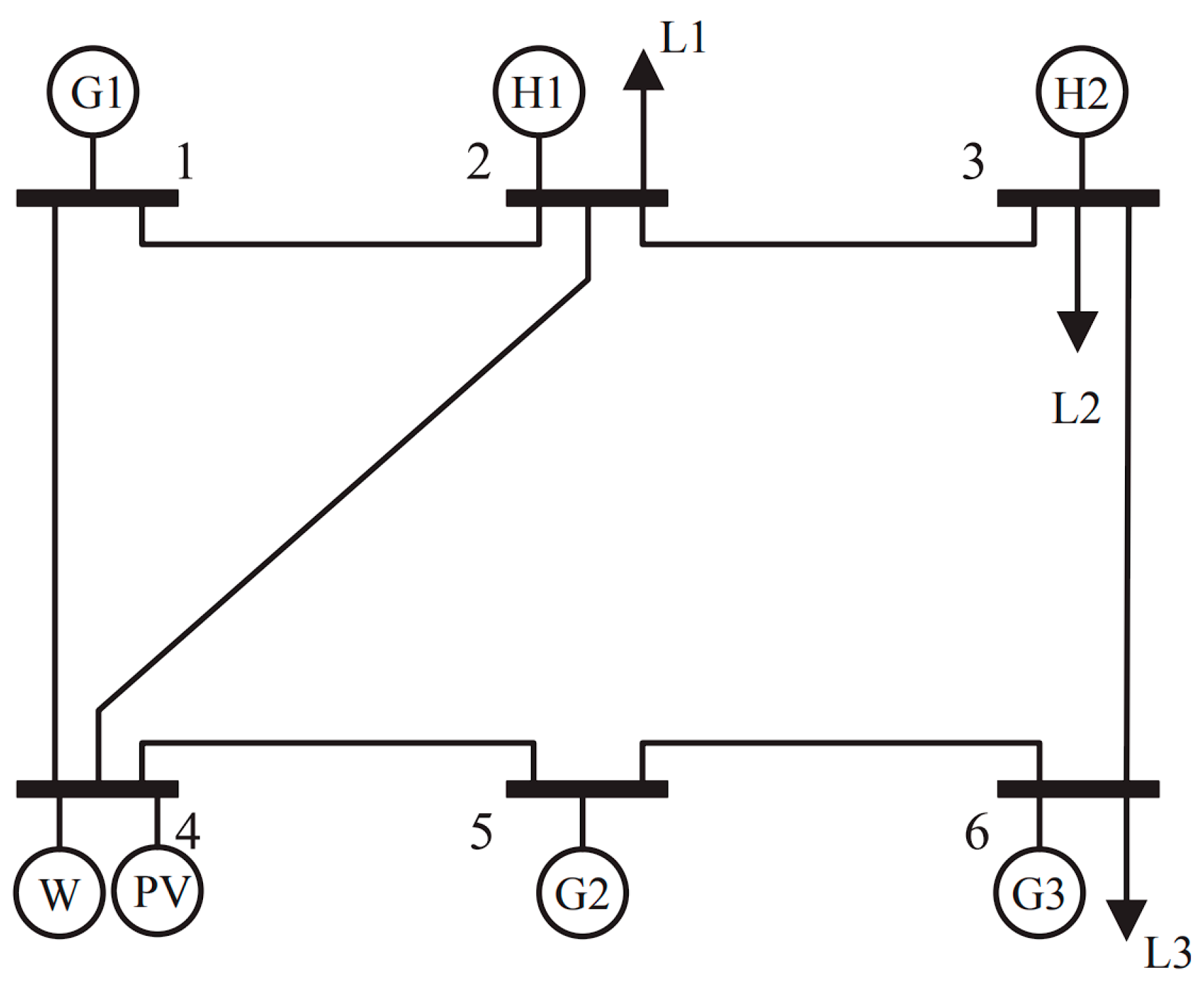
The effectiveness of the proposed day-ahead stochastic model was tested in a modified 6-bus power system [19]. The system node wiring diagram is shown in Figure 4. There are three conventional flexible thermal power units G1, G2, G3, two hydro units H1, H2, three loads L1, L2, L3, one wind power unit W, and one solar power unit PV.

The detailed parameters of these generators are shown in

Table 1. Thermal generation data.

Unit	Lower (MW)	Upper (MW)	Min Up/Down (h)	Ramp (MW/h)	Corrective (MW)
G1	50	150	8	100	80
G2	30	80	4	40	30
G3	10	50	3	40	15

,

Table 2. Fuel data.

Unit	a (MBtu)	b (MBtu/MWh)	c (MBtu/MW2h)	Start-Up Fuel (MBtu)	Fuel Price ($/Mbtu)
G1	0.0044	13.29	39	100	2.5
G2	0.0459	15.47	74.33	40	2.5
G3	0.0080	14.50	42	40	2.5

,

Table 3. Transmission line data.

Line	From	To	X (p.u.)	Flow Limite (MW)
L1	1	2	0.0370	200
L2	1	4	0.0160	200
L3	2	3	0.1015	175
L4	2	4	0.1170	175
L5	3	6	0.0355	175
L6	4	5	0.0370	200
L7	5	6	0.1270	200

and

Table 4. Hydro generator data.

Unit	H1	H2
Efficiency	6.197	6.465
H0	0.82679	0.58434
$\alpha$	4.2 × 10−4	1.15 × 10−3
Max discharge (m3)	2 × 105	2 × 105
Min discharge (m3)	0	0
Max volume (m3)	2.4 × 106	3.0 × 106
Min volume (m3)	1.0 × 106	1.2 × 106
Ramp (MW/h)	60	60
Min on/off time (h)	1	1
Lower bund (MW)	7	7
Upper (MW)	115	120
Nature inflow (m3)	1.5 × 105	5 × 104

, with data for the water-lined generators. The historical data and forecasted values of load, wind, and solar power generation are derived from Ref. [27]. The forecasted values of electrical load, wind, and solar generation are shown in Figure 5. $C_{\mathrm{R}}$ is set to 100 $\$/\mathrm{MW}$, and $C_l$ is set to 1000 $\$/\mathrm{MW}$. All case studies were solved using Gurobi 9.5.2 on a personal computer.

5.1. Deterministic Scheduling Case

5.1.1. Case 1

In this case, the dispatch model for the multi-source power system without DR can only dispatch for deterministic forecast values of electrical load and wind and solar generation.

Table 5. The operation results in case 1.

RES Penetration	Total Costs ($)	Loss of Load Penalty ($)	Curtailed RES Output Costs ($)	Thermal Power Generation Costs ($)
0	8,133,874.52	7,894,789.48	0	239,085.03
0.1	4,385,292.05	4,102,886.12	49,335.65	233,070.28
0.2	3,894,427.85	3,528,935.00	134,761.06	230,731.79
0.3	3,737,378.09	3,300,696.17	216,548.96	220,132.96
0.4	3,687,348.71	3,164,161.34	308,954.21	214,233.16
0.5	3,777,943.05	3,164,161.34	404,495.06	209,286.65
0.6	3,867,915.24	3,164,161.34	499,074.22	204,679.68

shows the impact of RES penetration on the associated dispatch costs in Case 1. The total costs consist of the loss of the load penalty, curtailed RES output costs, and power generation costs. With RES penetration increasing, total costs decrease and then increase mainly due to the loss of the load penalty and curtailed RES output cost. The load loss penalty decreases first but no longer decreases when the penetration rate is 0.4, and the curtailed RES output costs rise rapidly. The cost of thermal power generation has been decreasing, a trend attributed to the rising share of RES installations. This increase in the proportion of renewable sources reduces the generation costs for thermal power plants. When the RES penetration reaches 0.4, the limit of load balancing is reached. In the absence of DR, increasing the penetration of RES at this time will only increase curtailed RES output and reduce the output of thermal units without contributing to the source-load balance of the system and reducing loss of load.

Loss of load and curtailed RES under different RES penetration rates are shown in the Figure 6. The rate of loss of load decreased from 7.42% to 2.97% and then did not change again. Curtailed RES output rate continued to increase from 46.35% to 78.15%. Obviously, at low permeabilities, like 0.1, the curtailed RES output rate reached 46.35%. This is a very high value. These results show that in a new power system, the reduction in installed capacity of conventional units leads to a huge challenge in the source-load balance of the system and the absorption of RESs.

5.1.2. Case 2

The rate of flexible load participation in DR was set at 0.3. The influence of RES penetration on scheduling outcomes in case 1 is presented in

Table 6. The operation results in case 2.

RES Penetration	Total Costs ($)	Loss of Load Penalty ($)	DR Costs ($)	Curtailed RES Output Costs ($)	Thermal Power Generation Costs ($)
0.1	228,093.07	0	16,515.37	0	211,577.70
0.3	286,240.79	0	27,775.37	86,842.88	171,622.54
0.6	529,491.71	0	28,715.36	347,585.02	153,191.33

. We have examined three scenarios where flexible loads can be seamlessly adjusted to the optimal load profile, i.e., CDL. The results compared to case 1 show that CDL-based DR can effectively mitigate loss of load and reduce the curtailed RES output. When RES penetration is 0.1, the rate of curtailed RES output reduces from 46.35% in case 1 to 0%. Additionally, when RES penetration is 0.6, the rate of curtailed RES output reduces from 78.15% in case 1 to 54.43% because here there is a large RES output, but the load is small in comparison. Although it increases the DR costs, the total costs and the thermal power generation costs are much lower.

5.2. Stochastic Scheduling Case

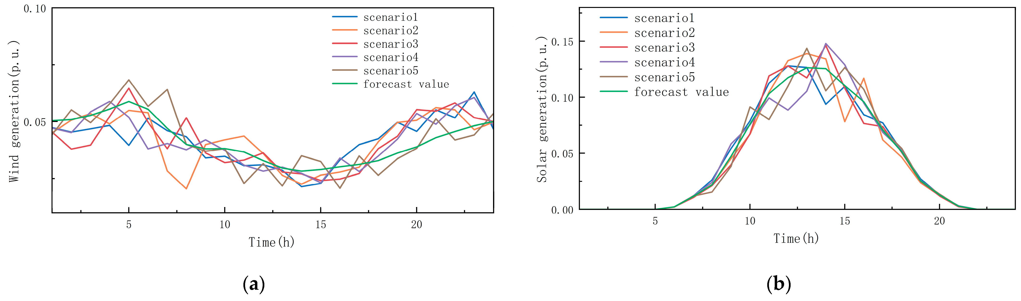
The complementary traits of wind-solar generations were modeled by using the Copula theory proposed in Section 4.1 to obtain 10,000 scenarios of wind-solar generations. Subsequently, we employed the fast-forward method presented in Section 4.2 to obtain reduced data sets of scenarios, providing 5 scenarios as a reasonable approximation of the 10,000 scenarios, as shown in Figure 7.

Table 7. The value of the weighting coefficients ${\rho }^{\xi }$.

$\mathbf{Scenario} \mathsf{\xi }$	1	2	3	4	5
${\rho }^{\xi }$	0.205	0.237	0.179	0.225	0.154

shows the value of the weighting coefficients ${\rho }^{\xi }$ in the objective function (39) obtained in scenario reduction.

In this section, we consider the uncertainties associated with wind and solar power generation, and the following scenarios are explored.

5.2.1. Case 3

Case 3 considers stochastic scheduling based on case 2. The rate of flexible load participating in DR was set at 0.3 and the RES penetration was set at 0.3. The customers adjust their load profiles as much as possible to improve the similarity metric $E$ in order to obtain more incentives. In case 3, the customer decision-making process was modeled by using the response evaluation model mentioned in Section 2.2. As described in Section 3, we obtained the value of $P_{l,t}^{\ast }$ and $P_{\mathrm{DR},t}^{\ast }$ in first stage. Then we calculated the value of $E\left(P_{l,t}^{\ast },P_{\mathrm{DR},t}^{\ast }\right)$. We can constrain the variable $P_{l,\mathrm{DR},t}^{\ast }$ by setting the value of $\Delta E$ as described in (6). For ease of discussion, we incremented the value of $\Delta E$ by 0.05. Thus, the value of the right-hand side of inequality (6) was increased by 0.05 from 0.75. Specially, because in practice it is impossible for $E$ to take the value 1, the last band was set to 0.99 instead of 1. Therefore, the similarity metric $E$ was divided into six bands from 0.75 to 0.99.

Figure 8 shows the shaping of the CDL profiles and actual customers’ load profiles at different response effects: during time periods 1 to 7, the units take on less load, and the CDL guides the customers to shift as much load as possible into that time period in the process of improving similarity $E$, boosting the load and thus filling in the valleys. Meanwhile, during time periods 9 to 16 and 17 to 23, the units take on more load, and the CDL guides the customers to shift as much load as possible out of that time period in the process of improving similarity metric $E$, reducing the load and thus achieving peak shaving.

The various costs at different values of $E$ are shown the

Table 8. The operation results in case 3.

$\mathit{E}$	Total Costs ($)	Loss of Load Penalty ($)	DR Costs ($)	Curtailed RES Output Costs ($)	Thermal Power Generation Costs ($)
0.75	786,499.26	347,849.23	9979.60	189,504.68	239,165.75
0.80	637,888.21	204,554.24	10,966.03	187,600.48	234,767.46
0.85	551,383.35	134,914.78	12,007.54	175,994.67	228,466.36
0.90	450,929.18	59,744.99	13,179.74	163,780.85	214,223.60
0.95	372,115.47	0	14,655.71	152,900.71	204,559.05
0.99	326,324.58	0	16,559.33	132,819.44	176,945.81

. Building on the observation from Table 8, the diminishing overall system costs with the increase in the similarity metric $E$ underscores the efficiency of DR mechanisms. As $E$ ascends, indicating higher customer participation in DR, it not only compensates for the DR costs incurred but also reduces operational and imbalance costs significantly. This trend demonstrates the value of aligning consumer behavior with system needs, leveraging flexible loads to enhance grid stability and integrate RES more effectively. This analysis suggests that a proactive DR strategy, supported by incentives and robust forecasting, can lead to a sustainable, cost-efficient energy system by mitigating the challenges posed by renewable intermittency and demand fluctuations. Therefore, the system can not only reduce the traditional generating units and use more RES units, which is conducive to the protection of the environment and reduce the use of fossil energy, but also obtain great economic benefits.

5.2.2. Case 4

In this case, with the aim to discuss the influence of forecasting errors in wind and solar generation, we reduced forecasting errors on the basis of case 3 by using the scenario modification method proposed in Ref. [19]. The error rate was set within 0.05. The forecasted wind and solar generation values and scenarios are displayed in Figure 9. In comparison with Figure 7, it can be observed that larger forecasting errors result in greater deviations in wind and solar generation, as well as higher levels of uncertainties. Forecasted errors in wind and solar generation were set to less than 0.05, and we discuss stochastic dispatch when the similarity metric $E$ was set to 0.9.

Figure 10 shows the results of unit commitment (UC) in case 3 and case 4. It should be noted that throughout the day hydro units H1, H2, along with thermal units G1, G3, remain in continuous operation. The UC solutions we obtained in case 3 differ from those in case 4. Due to the higher level of uncertainties in case 3, additional units must be activated to ensure the security of the system. In particular, there is a significant fluctuation in wind and solar generation in hour 12, during which the system shows insufficient ramping capacity. Therefore, thermal unit G2 provides enough ramping capabilities in case 3 by operating in additional hour 12, and the operation cost in case3 is USD 214,223.60, which is 11.37% more than that of case 4.

Table 9. The operation results in case 4.

Total Costs ($)	Loss of Load Penalty ($)	DR Costs ($)	Curtailed RES Output Costs ($)	Thermal Power Generation Costs ($)
418,091.17	49,232.03	13,179.74	163,324.90	192,354.50

shows the operation costs in case 4, and it is noted that the total costs, loss of load penalty, and thermal power generation costs are lower than those of case 3.

The base-case dispatches of H1 and H2 are increased from 3652.70 MWh in case 3 to 3751.45 MWh in case 4, and the dispatch of G3 was decreased from 1073.65 MWh in case 3 to 876.96 MWh in case 4. To ensure the system security under increased uncertainty and larger deviations in Case 3, an additional spinning reserve must be allocated to offset the fluctuations in wind and solar power generation from hydroelectric units. Consequently, less expensive hydro units operate at a suboptimal dispatch level in Case 3, but hydro units in case 4 are operating at a better dispatch level. As a result, the total costs are much lower in case 4.

6. Discussion

The simulation results in each case reveal the following insights: firstly, hydro units, as an effective regulatory resource, enhance the thermal-hydro-wind-solar system’s capacity to absorb RESs. However, hydro generation is influenced by hydrological conditions, seasonal variations, and other factors. Secondly, compared to scheduling models without DR, this study’s approach encourages consumers to adjust their electricity usage proactively, engaging more actively in DR. With increased participation in CDL-based DR, the system experiences significant peak shaving and valley filling effects, thereby enhancing the system’s reliability and economic efficiency. This, in turn, substantially facilitates the integration of a high proportion of new energy sources. Thirdly, the uncertainty of RES and the prediction errors in their generation affect operational costs. Larger prediction errors lead to increased levels of uncertainty, necessitating that hydro units provide more spinning reserve to compensate for the variability in wind and solar power generation. Additionally, more thermal units are required to ensure system reliability and stability. In summary, the proposed stochastic model offers a practical approach for identifying an optimal base-case dispatch strategy, thereby minimizing cost fluctuations amidst uncertainties.

As noted in Ref. [28], the expansion of the number of scenarios considerably increases the computational load.

Table 10. Computation time of cases 1–4.

Cases	1	2	3	4
Time (s)	4.09	4.78	458.59	145.41

shows the average computation time for all parameters in cases 1–4. It is observed that when not considering uncertainties in RESs, the computation time in case 1 is 4.09 s and that in case 2 is 4.78 s. When considering uncertainties in RESs, the computation time is increased significantly in case 3 and case 4. The computation time in case 3 with higher-level uncertainties is 458.59 s. It is about three times as long as in case 4. The reason is that more reserves are required to be turned on to balance real-time fluctuations in RES output by turning on additional units. Therefore, it needs longer time to obtain the solution in case 3.

7. Conclusions

We present a day-ahead stochastic scheduling method for day-ahead energy systems with CDL-based DR. The complementary traits between wind and solar power generation are modeled through Copula theory, and the Monte Carlo method is applied to simulate the wind and photovoltaic output errors to establish a set of stochastic scenarios for RES output. The objective function aims at minimizing the costs associated with RES integration, DR and load shedding, incorporating the uncertainties of cascaded hydroelectric units and RES to develop a day-ahead economic dispatch model that leverages multiple energy sources complementarily. Our model aims to obtain a dispatch solution with stable operating cost in the base case. This dispatch solution allows for the power system to operate under the forecasted base case and can safely redispatch all units in response to re-al-time fluctuations in RES output. Additionally, the model includes safety constraints to ensure more secure dispatch outcomes and effectively prevent flow overloading.

Our study demonstrates the potential of a day-ahead stochastic scheduling model with CDL to enhance the flexibility and efficiency of power systems. However, practical implementation faces several challenges: The deployment of this model requires advanced infrastructure capable of handling high volumes of data from diverse energy sources. Effective implementation relies on sophisticated communication protocols to ensure seamless interaction between the power system’s components. The protocols must ensure data integrity, security, and timeliness to facilitate the dynamic scheduling process. The regulatory environment plays a crucial role in the model’s implementation. Successful implementation requires coordination among all stakeholders, including power generators, grid operators, consumers, and regulatory bodies. Overcoming these challenges requires concerted efforts from all stakeholders and researchers.