
Rapid Investigation of Oil Pollution in Water-Combined Induced Fluorescence and Random Sample Consensus Algorithm
State Key Laboratory of Advanced Medical Materials and Devices, Department of Biomedical Engineering, Medical School, Tianjin University, Tianjin 300072, China
*
Author to whom correspondence should be addressed.
Sustainability 2024, 16(10), 3930; https://doi.org/10.3390/su16103930
Submission received: 6 April 2024
/
Revised: 2 May 2024
/
Accepted: 6 May 2024
/
Published: 8 May 2024
Abstract
:The global issue of oil spreading in water poses a significant environmental challenge, emphasizing the critical need for the accurate determination and monitoring of oil content in aquatic environments to ensure sustainable development of the environment. However, the complexity arises from challenges such as oil dispersion, clustering, and non-uniform distribution, making it difficult to obtain real-time oil concentration data. This paper introduces a sophisticated system for acquiring induced fluorescence spectra specifically designed for the quantitative analysis of oil pollutants. The paper involved measuring the fluorescence spectra across 20 concentration gradients (ranging from 0 to 1000 mg/L) for four distinct oil samples: 92# Gasoline, Mobil Motor Oil 20w-40, Shell 10w-40 engine oil, and Soybean Oil. The research focused on establishing a relationship model between relative fluorescence intensity and concentration, determined at the optimal excitation wavelength, utilizing the segmented Random Sample Consensus (RANSAC) algorithm. Evaluation metrics, including standard addition recovery, average recovery, relative error, and average relative error, were employed to assess the accuracy of the proposed model. The experimental findings suggest that the average recovery rates for the four samples ranged between 99.61% and 101.15%, with the average relative errors falling within the range of 2.04% to 3.14%. These results underscore the accuracy and efficacy of the detection methodology presented in this paper. Importantly, this accuracy extends to scenarios involving heavier oil pollution. This paper exhibits exceptional sensitivity, enabling precise detection of diverse oil spills within the concentration range of 0~1000 mg/L in water bodies, offering valuable insights for water quality monitoring and sustainable development of the environment.
1. Introduction
The expansive growth of oil extraction, transportation, and refining operations mirrors the rapid expansion of the global economy. However, this widespread development has led to a disturbing increase in incidents related to crude oil pollution, stemming from fuel oil leaks, spills from offshore drilling platforms, and discharges from oil tankers [1]. According to the statistics of the International Tanker Owners Pollution Federation (ITOPF) in the United States, there have been over 700 tons of large-scale oil spills every year over the past half-century. The total volume of oil lost to the environment from tanker spills in 2023 was approximately 2000 tons. In April 2021, the Panamanian general cargo ship “Sea Justice” collided with the Liberian tanker “A Symphony” in the waters off Qingdao, Shandong Province. This collision resulted in a spill of approximately 9400 tons of cargo oil into the sea [2], causing extensive oil spill pollution along hundreds of kilometers of coastline. Furthermore, leaks from offshore drilling platforms significantly contribute to the persistence of residual oil pollution in water bodies.
Oil spills create a layer on the surface of seawater, impeding gas exchange between air and seawater. This interference leads to hypoxia and the death of marine organisms, weakening the self-purification ability of the ocean [3,4]. Petroleum pollutants, characterized by petroleum hydrocarbons, toluene, and other hazardous components [5], directly harm the quality of water and infiltrate the terrestrial food chain via the enrichment of aquatic organisms. Despite efforts to enhance safety, maritime accidents continue to pose a major threat. In recent years, serious accidents have occurred frequently, resulting in severe consequences [6] and seriously hindering the sustainable development of the environment.
In the face of these environmental risks and challenges, the development of a technique capable of swift and precise detection of oil pollutants in water bodies is imperative for the preservation of both marine and terrestrial ecosystems [7,8]. Such a method would not only enable prompt responses to oil-related incidents but also contribute significantly to proactive measures in environmental protection. The urgency of this need is underscored by the potential far-reaching consequences of unchecked oil pollution on both ecosystems and human well-being.
Currently, technologies for detecting oil spills at sea encompass a range of advanced methods. These include infrared spectroscopy measurement technology [9,10,11], microwave radiometry [12], microwave triangulation method, dual-light interference method [13], laser ultrasound method, and UV-induced fluorescence [14,15] in remote sensing, among others. In prior research, light-induced fluorescence (LIF) technology has been extensively employed in the detection field due to its capacity for rapid and non-destructive analysis of target samples. Recognized as one of the most effective techniques for detecting oil spills on the sea’s surface [16], LIF technology’s applicability has been acknowledged by scientific researchers from the United States, Germany, France, and Canada, who were pioneers in realizing its potential for detecting sea surface oil spills [17]. As early as 1971, Bristow [18] and colleagues proposed the installation of a fluorescence radar detection system on an airplane to facilitate the detection of oil spills on the sea surface.
In recent years, there have been more and more researchers paying more attention to LIF technology in the field of chemical analysis. Sami D. Alaruri [19] employed the LIF lidar system to measure the fluorescence intensity of both fresh and weathered oil samples. They combined this data with a principal component algorithm to successfully identify and classify unknown oil samples. Yongqiang Cui and Deming Kong [20] introduced an inversion algorithm that integrates Raman scattering light and fluorescence signals. This approach evaluates the thickness of oil spills on the sea surface, building upon the method proposed by Hoge et al. [21]. By addressing significant errors in Hoge et al.’s integral inversion algorithm based on Raman scattering light for thin oil film thickness evaluation, Cui and Kong [20] enhanced the accuracy of the oil film thickness inversion results. Zhikun Chen and Rui Guo [22] employed laser-induced fluorescence technology in conjunction with a characteristic parameter extraction method and curve-fitting techniques. This combination facilitated qualitative measurement of 10 mg oil pollutants, as well as qualitative and quantitative measurement in the lower concentration range of 10 mg/L or less.
Nevertheless, the current application of laser-induced fluorescence technology encounters non-linear challenges and huge deviations for large-scale oil concentration; particularly, the algorithm models are usually limited by the weak fluorescent intensity and non-sensitive when the oil concentration is greater than 50 mg/L. Both the variability in fluorescent groups emitted by different oil species and the fluorescence burst effect can contribute to the inadequate robustness of a unified quantitative model for predicting oil spill concentration and lead to diminished accuracy in oil spill concentration detection.
In response to these challenges, this paper proposed a method combining light-induced fluorescence spectroscopy (LIFS) with a segmented RANSAC algorithm for oil concentration determination in water, as well as developing a LIFS acquisition system. The experimental design breaks through the constraints of the limited scale of pollution concentration, extending to 1000 mg/L from 10 mg/L in most previous studies. Experimental tests have been carried out on oil contamination samples of 92# gasoline, Shell 10w-40 motor oil, and Soybean Oil, ranging from 0 mg/L to 1000 mg/L. Fluorescence spectra of these samples were captured across 190~600 nm, and spectra smoothing and baseline correction were performed to obtain relative fluorescence intensity corresponding to the optimal emission wavelength. Moreover, it is rather The RANSAC algorithm than PLS employed to fit the concentration and relative fluorescence intensity, which resulted in the lowest derivation to each oil species prepared. This innovative approach can improve the accuracy and applicability of laser-induced fluorescence technology for the determination of oil spills in water, which is beneficial for water quality monitoring and sustainable development of the environment.
To summarize, our main contributions are as follows:
- Introduces an innovative analytical approach by integrating Laser-Induced Fluorescence (LIF) with the Random Sample Consensus (RANSAC) algorithm.
- Overcomes the constraints associated with lower oil concentration scales ranging from 0 to 10 mg/L, expanding the traditional oil-in-water detection dataset.
- Exhibits exceptional sensitivity, enabling precise detection of diverse oil spills within the concentration range of 0~1000 mg/L in water bodies.
2. Materials and Methods
2.1. Experimental Samples
In the realm of water pollution, heavy oil spills dominate marine environments. However, in the context of river pollution and urban sewage, light oil leaks contribute to water pollution [23]. Consequently, acquiring laser-induced fluorescence spectra for both light and heavy oils becomes paramount in the monitoring of water pollution.
To emulate the real-world application of oil spill pollution in natural surface water, this investigation involved the careful selection of four distinct oil samples, accompanied by the collection of corresponding water samples for experimental preparation. The water samples were systematically collected from Jingye Lake at Tianjin University, situated in the Nankai District of Tianjin, China, spanning the period from July to October 2023. The longitude and latitude of Jingye Lake are shown in Figure 1.
The chosen oil pollutants, namely 92# Gasoline, Mobil Motor Oil 20w-40, Shell Oil 10W-40, and Soybean Oil, were deliberately introduced into the natural water samples at predetermined concentrations. For each pollutant, concentrations were meticulously selected within the pertinent range to assess the model’s efficacy in detecting them. The concentration range for the four selected oil samples spanned from 0 to 1000 mg/L, with 20 concentration gradients selected. Each concentration sample was measured 10 times, resulting in a total of 800 mixing experiments conducted.
In the experimental configuration, four 100 mL volumetric flasks were employed, each containing 0.1 g of the respective oil samples, resulting in standard solutions with a mass concentration of 1000 mg/L. N-hexane was chosen as the extractant for isolating oil samples from the collected water samples. To create a concentration gradient in the samples, various volumes of the standard solution were mixed with water in different series of volumetric flasks. This step facilitated the generation of samples with diverse concentrations. The specific volume adjustments of the standard solution and water were made to achieve 20 concentration gradients for each oil sample, as outlined in Table 1.
2.2. Experimental Setup
Figure 2 below illustrates the oil spill detection system constructed by this paper according to principles of induced fluorescence technology. A pulsed xenon lamp, covering the range of 185~2000 nm, serves as the excitation light source. This excitation light is converged and directly projected on the sample, inducing ultraviolet fluorescence due to fluorophores like aromatic hydrocarbon, anthracene, etc., particularly from those oil scratches suspending and dissolved in the water. In the vertical of the direction incident light, another converging lens was embedded, and a UV glass fiber with a 600 µm core diameter was fixed to collect the emission fluorescence light as much as possible.
To improve the detection efficiency of weak fluorescence signals and reduce the interference of environmental light on these signal detections, this paper employs the QE PRO high-sensitivity spectrometer from Ocean Optics. An extended integration time of 200 milliseconds is utilized to bolster the spectrometer’s capacity to detect weak signals. Paramount to this research is the use of the XFS-II high-output xenon lamp, an excitation light source independently developed by Tianjin University. This light source is capable of emitting flickering light at a predetermined frequency, which can be synchronized with the spectrometer’s operation via programmatic control. It has been determined that each procedural step outlined is integral to the process of laser-induced fluorescence measurement; omission of any step could lead to measurement failure. In the practical execution, the spectra are averaged after ten flashes to achieve more reliable data. Each spectral acquisition process is conducted over approximately 2 s to ensure data stability and accuracy.
2.3. Principles of the RANSAC Algorithm
Normally speaking, spectral data are statistically PLS fitted to the gradients vs. intensity peaks at contain wavelengths as the previous report [24], but it is discovered that there is non-linear and greater dispersed when the oil concentration is greater than 10 mg/L and the peaks are not constant when the oil becomes thicker. Finally, we chose a RANSAC algorithm for the prediction of oil spill investigation.
Fischler and Bolles proposed the RANSAC algorithm early in 1981 [25]. The logic of the RANSAC algorithm assumes that the collected sample dataset contains both correct data and an abnormal dataset far from the normal range of the sample dataset. The RANSAC algorithm is designed to estimate mathematical errors from such a mixed data set, using an iterative approach to find a model parameter most suitable for describing the correct data. Figure 3 below illustrates the data flow of the RANSAC algorithm [26,27].
In the computational process of the RANSAC algorithm, several parameters need determination, including a threshold for assessing the number of inliers, a suitably reasonable count of inliers , and the number of iterations . The value of can be deduced from theoretical outcomes. When determining the threshold and the reasonable count of inliers , denotes the probability that points randomly chosen from the dataset in the iteration process are all inliers, while signifies the probability of selecting a single inlier point from the dataset on each iteration, with = the number of inliers divided by the total number of datasets.
Assuming the estimation model requires the selection of points, where is the probability that all points are local inliers then represents the probability that at least one of the points is an outlier, indicating the potential estimation of a flawed model from the dataset. The probability that the algorithm will never select n points that are all local inliers is denoted by , which is equivalent to . Taking the logarithm of both sides yields the number of iterations [28]:
The selection of the threshold is crucial as it directly impacts the categorization of outliers and outliers. Opting for a smaller value may lead to the omission of valid points a larger value might mistakenly identify outliers or erroneous points as valid. In response to this challenge, this paper employs the Mean Absolute Deviation (MAD), denoted as , to estimate the data variance [29]. The expression for is given by
Here, median denotes the median function for array calculation, |·| represents the absolute value, and and are the positions of the data subset. The threshold is set as the absolute median difference in the experimental data, subsequently used in other experimental datasets.
For this analysis of the spectral dataset, errors or deviations rising from the environmental interference, spectrometer instruments, flashlight amplitude vibrations, or flasks cleaning can be taken into consideration as an abnormal dataset, compared with the traditional least squares algorithm at several given wavelengths, the use of the RANSAC algorithm is obviously superior to eliminate the interference and make the results more robust and reliable.
3. Results and Discussion
3.1. Fluorescence Spectral Analysis
Figure 4 below presents the initial fluorescence spectra of 92# Gasoline, Mobil Motor Oil 20w-40, Shell Oil 10w-40, and Soybean Oil at various concentrations. These spectra were acquired within the range of 200 nm to 600 nm using the fluorescence spectral acquisition system. In the four subfigures of Figure 4, the horizontal coordinates denote the wavelengths, while the vertical coordinate represents the magnitude of the fluorescence intensity. The spectrograms underwent baseline correction and smoothing processes, enhancing the clarity and reliability of the data. These refined fluorescence spectra enable the extraction of distinctive fluorescence signals corresponding to varying concentrations of different types of oils.
As depicted in Figure 4 and Figure 5, the fluorescence emission spectra of the four oils spanned the range of 200 nm to 600 nm, and the peak distribution is between 280 and 350 nm. Notably, the fluorescence intensity of each oil exhibited a continuous increase corresponding to the rise in oil concentration within the detected range of 0 to 1000 mg/L.
3.2. Concentration Prediction Modeling
During the measurement process of lower mass concentration solutions, the fluorescence intensity measured by the system demonstrates a linear relationship with the mass concentration of the solution, given by the equation [30] as follows:
Here, represents the fluorescence intensity, and is the fluorescence quantum yield. denotes the excitation intensity, signifies the mass concentration of the solution, is the molar absorption coefficient, and represents the transmitted optical path.
The outlined expression (Equation (3)) elucidates the direct proportionality between the fluorescence intensity and the mass concentration of the solution under constant excitation intensity. This linear relationship is pivotal in the quantitative assessment of lower mass concentration solutions, providing a basis for accurate measurements and analysis in fluorescence spectroscopy. The parameters within the equation collectively contribute to the sensitivity and reliability of the analytical method, forming a critical foundation for understanding and characterizing the fluorescence behavior of the tested solutions.
However, when the concentration of quantitative detection exceeds a specific range, interactions among fluorescent molecules in the excited state and those in the ground state may result in a decrease in fluorescence intensity or complete disappearance [31]. This phenomenon is referred to as the internal quenching of fluorescence.
Analyzing the experimental data reveals that within the detected range of 0 to 1000 mg/L, the mass concentration of the sample and its corresponding fluorescence intensity do not exhibit a purely linear relationship. The linear correlation between the mass concentration of the sample and its fluorescence intensity may vary in the high-concentration band, the middle-concentration band, and the low-concentration band. Given the diverse internal groups and fluorescence burst effects associated with different oil species, this paper adopts a flexible approach, selecting segmentation points to delineate the concentration detection range. This facilitates the quantitative analysis of each oil species using the RANSAC algorithm.
Fitting curves were generated based on 600 sets of induced fluorescence spectroscopy data for the four types of oils (92#Gasoline, Mobil Motor Oil 20w-40, Shell Oil 10w-40, and Soybean Oil) at varying mass concentrations within the database. Figure 6, Figure 7, Figure 8 and Figure 9 illustrate the fitted curves depicting the relationship between mass concentration and relative fluorescence intensity for 92#Gasoline, Mobil Motor Oil 20w-40, Shell Oil 10w-40, and Soybean Oil, respectively. In each subfigure of these four figures, the horizontal axis represents mass concentration, while the vertical axis represents the magnitude of fluorescence intensity. Figure 6, Figure 7, Figure 8 and Figure 9 elucidate the connection between relative fluorescence intensity and sample concentration. Simultaneously, the segmented fitted curves for these four oils serve as prediction models for their respective mass concentrations.
3.3. Detection Limits of Oil Pollutants
The Limit of Detection (LOD) signifies the minimum concentration that an analytical method can discern within a specified range [32]. The computation method for LOD is articulated as follows:
The expression for the minimum measurable signal is represented as
Here, denotes the mean of spectral signals from multiple blank samples, is the standard deviation of spectral signals from multiple blank samples, and m is the slope of the calibration curve. As this article employs piecewise linear regression for fitting the standard curve, the slope of the standard curve in the low concentration range is specifically chosen.
The concentration corresponding to constitutes the LOD formula:
In this context, k is a constant selected based on the confidence level [33]. For spectral chemical analysis, k = 3 is adopted to ensure a confidence level of 90%. The detection limits for four types of oils are calculated using Equation (5) and are presented in Table 2.
From the observations in Table 2, it is evident that there is a strong correlation (r ≥ 0.99) between the oil concentration in water and fluorescence intensity in the standard curves of various oil pollutants. By the definition of the detection limit, the calculated detection limits for each oil type are as follows: 0.8 mg/L for 92# gasoline, 0.9 mg/L for Mobil engine oil 20w-40, 0.07 mg/L for Shell 10w-40, and 0.5 mg/L for Soybean Oil. The detection limit range for measuring the concentration of these four types of oil products falls between 0.07 and 0.9 mg/L, aligning well with the requirements for rapid detection and daily monitoring of water pollution.
These calculated detection limits underscore the sensitivity of the proposed method, ensuring its capability to discern low concentrations of oil pollutants in water samples. The robust correlation observed in the standard curves further validates the reliability of the analytical approach, supporting its potential for effective application in the swift and routine assessment of water quality in terms of oil pollution. The established detection limits within this concentration range provide a practical framework for addressing the specific needs of water quality monitoring, offering a valuable tool for environmental management and protection.
3.4. Predictive Model Evaluation Indicators
Based on the obtained concentration prediction models for the four oils, for the sample solutions with unknown concentrations of known oils, the relative fluorescence intensities of the samples were obtained from the spectrograms of the samples collected by the system to predict their mass concentrations. At the same time, the accuracy of the prediction results could be evaluated.
To assess the precision and dependability of the model outcomes, several pertinent statistical parameters and quality metrics are introduced. Primarily, these encompass the Blank Recovery Rate, Average Recovery Rate, Relative Error of Prediction (REP), and Mean Relative Error (MRE), all instrumental in evaluating the efficacy of the analytical methodology.
The Blank Recovery Rate serves as a measure of the model’s ability to accurately recover known concentrations in blank samples. Meanwhile, the Average Recovery Rate provides an overall assessment of the model’s accuracy in predicting concentrations across various samples.
The Relative Error of Prediction (REP) is employed to quantify the difference between the predicted values and the actual concentrations, offering insights into the model’s predictive precision. Complementing REP, the Mean Relative Error (MRE) calculates the average relative discrepancies, providing a consolidated measure of the overall predictive accuracy.
Introducing these statistical parameters and quality metrics facilitates a comprehensive evaluation of the analysis method, ensuring a thorough understanding of the model’s performance characteristics.
① Blank Recovery Rate
The spiked recovery rate serves as a crucial methodology for validating the accuracy of measurements, typically categorized into two components: blank spiked recovery rate and sample spiked recovery rate. This analytical approach involves the intentional addition of a known quantity of the analyte to samples, allowing the assessment of the method’s precision and reliability.
The blank spiked recovery rate assesses the accuracy of measurements in the absence of a sample matrix, while the sample spiked recovery rate evaluates accuracy within the context of real-world samples. An optimal spiked recovery rate aligns closely with 100%, indicating a high level of accuracy in the measurement method. Conventionally, this recovery rate is managed within the controlled range of 80% to 120%, ensuring the reliability and robustness of the measurement process.
The blank spiking recovery in this concentration prediction model is the ratio of the predicted result to the theoretical value obtained by adding a quantitative amount of oil to the solvent and analyzing and predicting its concentration by systematically detecting its relative fluorescence intensity. The formula for the recovery rate can be expressed as
In the above equation, is the spiked recovery of the th sample concentration of the same oil, is the analytical model predicted concentration of the th sample of the same oil, and is the configured concentration of the th sample of the same oil.
② Average Recovery Rate
This is the average of the spiked recoveries for all concentration samples of the same oil type.
In the above equation, is the Average Recovery Rate, is the spiked recovery of the th sample concentration of the same oil, and N represents the number of predicted samples.
③ Relative Error of Prediction (REP)
The relative error can be used to express the magnitude of the difference between the predicted and accurate concentrations. The formula can be expressed as
In the above equation, denotes the actual concentration of the substance in the th sample, and represents the predicted concentration of the substance in the th sample.
④ Mean Relative Error (MRE)
The Mean Relative Error (MRE) is a statistical metric calculated as the average of the relative errors derived from the regression of identical substances across various samples. Its formulation is expressed as follows:
In the above equation, denotes the actual concentration of the substance in the th sample, represents the predicted concentration of the substance in the th sample, and N is the number of predicted samples.
This parameter provides a consolidated assessment of the relative errors across multiple samples, offering a comprehensive measure of the overall predictive accuracy of the regression model.
3.5. Analysis of Forecast Results
Table 3 displays the comparison between the detection concentration values using the method we proposed and the actual concentration values of four oil pollutants (Due to the space limitations, only partial results are shown here). According to Table 3, the method exhibits accuracy, demonstrating an overall commendable performance.
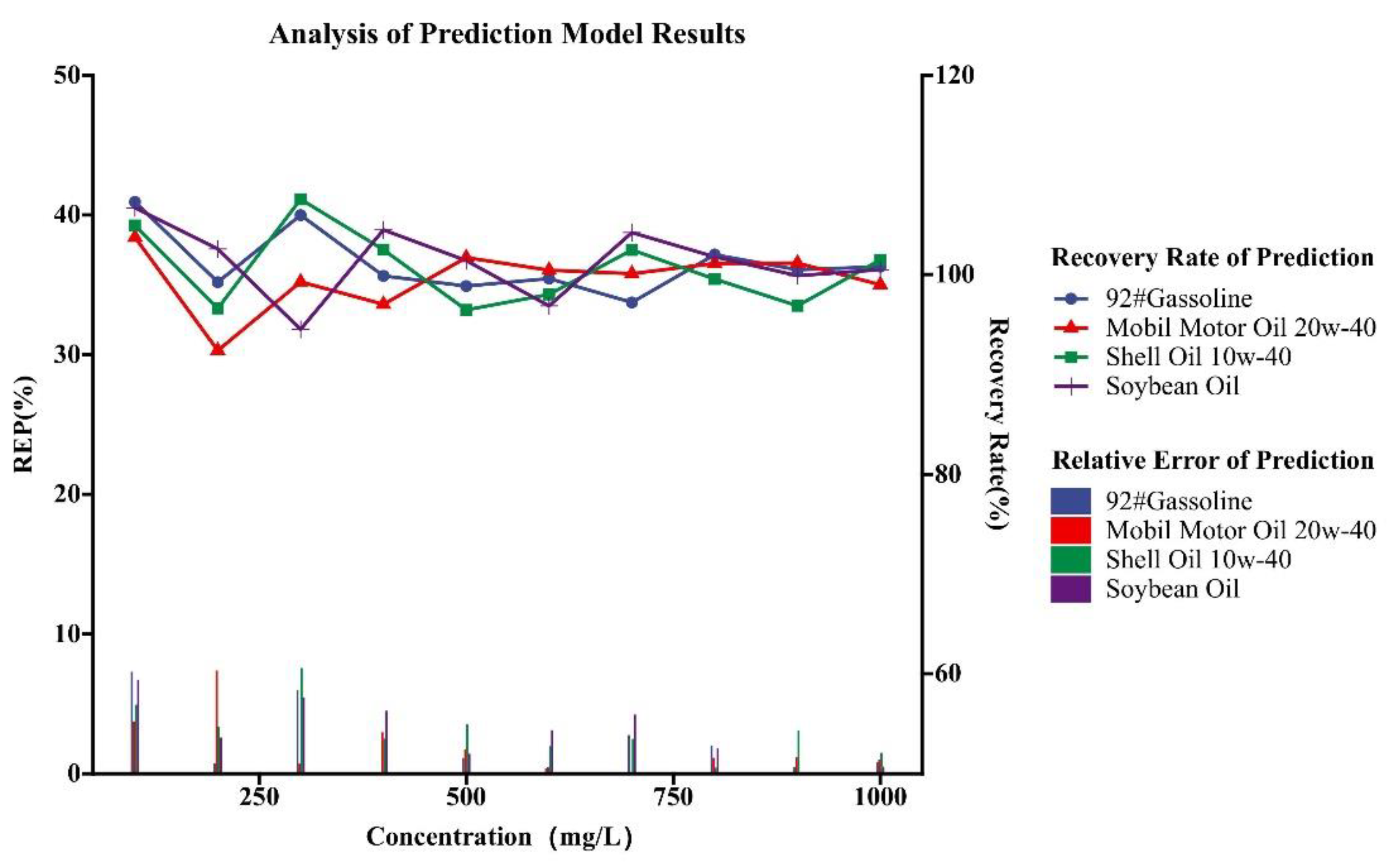
Considering the inadequacy of conventional methods in detecting oil in water at high concentrations, Figure 10 presents the analysis outcomes of the predicted concentration recovery rates and relative error of prediction for high concentrations (100~1000 mg/L) of four oil types (92#Gasoline, Mobil Motor Oil 20w-40, Shell Oil 10w-40, and Soybean Oil) using the predictive analysis model combining Laser-Induced Fluorescence and the RANSAC algorithm. Among them, the horizontal axis delineates the concentration of oil samples, while the vertical axis indicates the recovery rate and the relative error, respectively. Each plotted line traces the trajectory of the blank spiked recovery rate across varying concentrations for different types of oil. The inferior portion of Figure 10 presents the relative error associated with various oil types and their corresponding concentrations.
The spectral model, as presented in Figure 10, has been meticulously constructed via the integration of spectra utilizing the segmented RANSAC algorithm, which has proven to be a robust and effective method for enhancing predictive accuracy, particularly within the high-concentration band. This model’s performance is characterized by a commendable predictive efficacy, as evidenced by the recovery rates and relative errors associated with the high-concentration predictions for various oil samples.
For 92# Gasoline, the model demonstrates a recovery rate that varies from 97.23% to 107.30%, with an impressive average recovery rate of 101.15%. The relative error of these predictions is kept within a narrow range, from 0.11% to 7.30%, culminating in an average relative error of 2.17%. This level of precision is indicative of the model’s reliability in accurately estimating the mass concentration of gasoline at elevated concentrations.
Similarly, Mobil Motor Oil 20w-40 exhibits a recovery rate that ranges from 92.41% to 103.75%, with an average recovery rate of 99.61%. The relative error is also well-contained, fluctuating between 0.11% and 7.39%, resulting in an average relative error of 2.04%.
The performance of the model with Shell Oil 10w-40 at high concentrations is equally noteworthy, with a recovery rate spanning from 96.48% to 107.57% and an average recovery rate of 100.59%. The relative error is slightly higher, ranging from 0.43% to 7.57%, but still maintains an average relative error of 3.14%, which is within acceptable limits for practical applications.
In the case of Soybean Oil, the model’s high-concentration predictions show a recovery rate between 94.53% and 106.71%, with an average recovery rate of 100.94%. The relative error is kept within a tight range of 0.09% to 6.71%, averaging 3.04%, which is a testament to the model’s versatility and adaptability across different types of oils.
4. Conclusions
This paper introduces an innovative and robust method for the quantitative analysis of oil pollution by fusing Laser-Induced Fluorescence with the RANSAC algorithm. Underpinning this paper is a dataset of 800 spectral measurements, encompassing four varieties of oil products at varying concentrations, acquired utilizing an aquatic oil detection system. The methodology employs a segmented RANSAC algorithm to construct a predictive model for oil concentration in water, yielding four distinct models adept for concentrations spanning from 0 to 1000 mg/L. An in-depth evaluation of the model’s predictive efficacy across diverse concentration gradients was conducted. The findings demonstrate average recovery rates for all samples between 99.61% and 101.15% and average relative errors between 2.04% and 3.14%. These outcomes underscore the precision and reliability of the proposed detection technique, offering significant contributions to the realms of water quality monitoring and the advancement of environmental sustainability.
Author Contributions
H.W.: Conceptualization, Methodology, Software, Investigation, Formal Analysis, Writing—Original Draft; Z.W.: Data Curation, Data Analysis; Y.Z.: Resources, Writing—Review and Editing. All authors have read and agreed to the published version of the manuscript.
Funding
This research was funded by the National Natural Science Foundation of China, grant number 42177439.
Institutional Review Board Statement
Not applicable.
Informed Consent Statement
Not applicable.
Data Availability Statement
The raw data supporting the conclusions of this article will be made available by the authors upon request.
Acknowledgments
We acknowledge the support from the State Key Laboratory of Advanced Medical Materials and Devices of Tianjin University.
Conflicts of Interest
The authors declare no conflicts of interest.
References
- Elsheref, M.; Messina, L.; Tarr, M.A. Photochemistry of oil in marine systems: Developments since the Deepwater Horizon spill. Environ. Sci.-Process. Impacts 2023, 25, 1878–1908. [Google Scholar] [CrossRef] [PubMed]
- Gong, B.W.; Zhang, H.J.; Wang, X.; Lian, K.; Li, X.; Chen, B.; Wang, H.; Niu, X. Ultraviolet-induced fluorescence of oil spill recognition using a semi-supervised algorithm based on thickness and mixing proportion-emission matrices. Anal. Methods 2023, 15, 1649–1660. [Google Scholar] [CrossRef] [PubMed]
- French-McCay, D.P.; Parkerton, T.F.; de Jourdan, B. Bridging the lab to field divide: Advancing oil spill biological effects models requires revisiting aquatic toxicity testing. Aquat. Toxicol. 2023, 256, 106389. [Google Scholar] [CrossRef] [PubMed]
- Nilén, G.; Larsson, M.; Hyötyläinen, T.; Keiter, S.H. A complex mixture of polycyclic aromatic compounds causes embryotoxic, behavioral, and molecular effects in zebrafish larvae (Danio rerio), and in vitro bioassays. Sci. Total Environ. 2024, 906, 167307. [Google Scholar] [CrossRef] [PubMed]
- Asif, Z.; Chen, Z.; An, C.; Dong, J. Environmental Impacts and Challenges Associated with Oil Spills on Shorelines. J. Mar. Sci. Eng. 2022, 10, 762. [Google Scholar] [CrossRef]
- Cui, Y.Y.; Kong, D.M.; Kong, L.; Wang, S. Excitation emission matrix fluorescence spectroscopy and parallel factor framework-clustering analysis for oil pollutants identification. Spectrochim. Acta Part A Biomol. Spectrosc. 2021, 253, 119586. [Google Scholar] [CrossRef] [PubMed]
- Jaén-González, L.; Aliaño-González, M.J.; Ferreiro-González, M.; Barbero, G.F.; Palma, M. A Novel Method Based on Headspace-Ion Mobility Spectrometry for the Detection and Discrimination of Different Petroleum Derived Products in Seawater. Sensors 2021, 21, 2151. [Google Scholar] [CrossRef]
- Zhang, Z.H.; Yan, L.; Jiang, X.; Ding, J.; Zhang, F.; Jiang, K.; Shang, K. Exploring the Potential of Optical Polarization Remote Sensing for Oil Spill Detection: A Case Study of Deepwater Horizon. Remote Sens. 2022, 14, 2398. [Google Scholar] [CrossRef]
- Jiao, J.N.; Lu, Y.C.; Hu, C.; Shi, J.; Sun, S.; Liu, Y. Quantifying ocean surface oil thickness using thermal remote sensing. Remote Sens. Environ. 2021, 261, 112513. [Google Scholar] [CrossRef]
- Arslan, N.; Nezhad, M.M.; Heydari, A.; Garcia, D.A.; Sylaios, G. A Principal Component Analysis Methodology of Oil Spill Detection and Monitoring Using Satellite Remote Sensing Sensors. Remote Sens. 2023, 15, 1460. [Google Scholar] [CrossRef]
- Guo, G.; Liu, B.X.; Liu, C. Thermal Infrared Spectral Characteristics of Bunker Fuel Oil to Determine Oil-Film Thickness and API. J. Mar. Sci. Eng. 2020, 8, 135. [Google Scholar] [CrossRef]
- Dala, A.; Arslan, T. In Situ Sensor for the Detection of Oil Spill in Seawater Using Microwave Techniques. Micromachines 2022, 13, 536. [Google Scholar] [CrossRef] [PubMed]
- Lu, Y.C.; Tian, Q.J.; Li, X. The remote sensing inversion theory of offshore oil slick thickness based on a two-beam interference model. Sci. China-Earth Sci. 2011, 54, 678–685. [Google Scholar] [CrossRef]
- Fingas, M. The Challenges of Remotely Measuring Oil Slick Thickness. Remote Sens. 2018, 10, 319. [Google Scholar] [CrossRef]
- Jafarzadeh, H.; Mahdianpari, M.; Homayouni, S.; Mohammadimanesh, F.; Dabboor, M. Oil spill detection from Synthetic Aperture Radar Earth observations: A meta-analysis and comprehensive review. GI Sci. Remote Sens. 2021, 58, 1022–1051. [Google Scholar] [CrossRef]
- Fingas, M.; Brown, C.E. A Review of Oil Spill Remote Sensing. Sensors 2018, 18, 91. [Google Scholar] [CrossRef]
- Lennon, M.; Babichenko, S.; Thomas, N.; Mariette, V.; Mercier, G.; Lisin, A. Detection and mapping of oil slicks in the sea by combined use of hyperspectral imagery and laser-induced fluorescence. EARSeL eProceedings 2006, 5, 120. [Google Scholar]
- Rayner, D.M.; Szabo, A.G. Time-resolved Laser Fluorosensors-Laboratory Study of Their Potential in the Remote Characterization of Oil. Appl. Opt. 1978, 17, 1624–1630. [Google Scholar] [CrossRef] [PubMed]
- Alaruri, S.D. Multiwavelength laser induced fluorescence (LIF) LIDAR system for remote detection and identification of oil spills. Optik 2019, 181, 239–245. [Google Scholar] [CrossRef]
- Cui, Y.Q.; Kong, D.M.; Ma, Q.; Xie, B.; Zhang, X.; Kong, D.; Kong, L. Algorithm Research on Inversion Thickness of Oil Spill on the Sea Surface Using Raman Scattering and Fluorescence Signal. Spectrosc. Spectr. Anal. 2022, 42, 104–109. [Google Scholar]
- Hoge, F.E. Oil film thickness using airborne laser-induced oil fluorescence backscatter. Appl. Opt. 1983, 22, 3316–3318. [Google Scholar] [CrossRef]
- Chen, Z.K.; Guo, R.; Cheng, P.F. Application of LIF Technology-Based Spectral Feature Extraction in Oil Detection. Laser Optoelectron. Prog. 2020, 57, 133002. [Google Scholar] [CrossRef]
- Hong, J.J.; Wang, Z.H.; Li, J.; Xu, Y.; Xin, H. Effect of Interface Structure and Behavior on the Fluid Flow Characteristics and Phase Interaction in the Petroleum Industry: State of the Art Review and Outlook. Energy Fuels 2023, 37, 9914–9937. [Google Scholar] [CrossRef]
- Köpplin, J.; Bednarz, L.; Hagemeier, T.; Thévenin, D. Fluorescence Imaging Methodology for Oil-in-Water Concentration Measurements. Chem. Eng. Technol. 2021, 44, 1343–1349. [Google Scholar] [CrossRef]
- Fischler, M.A.; Bolles, R.C. Random sample consensus: A paradigm for model fitting with applications to image analysis and automated cartography. Commun. ACM 1981, 24, 381–395. [Google Scholar] [CrossRef]
- Zhou, C.L.; Zhu, H.H.; Li, X. Research and application of robust plane fitting algorithm with RANSAC. Comput. Eng. Appl. 2011, 47, 177–179, 182. [Google Scholar]
- Xie, S.S.; Wang, Z.Q.; Huang, H. Applications of random sample consistency algorithm on laser spectroscopy. Laser Technol. 2017, 41, 133–137. [Google Scholar]
- Raguram, R.; Chum, O.; Pollefeys, M.; Matas, J.; Frahm, J.M. USAC: A Universal Framework for Random Sample Consensus. IEEE Trans. Pattern Anal. Mach. Intell. 2013, 35, 2022–2038. [Google Scholar] [CrossRef] [PubMed]
- Guan, H.Q.; Chen, Z.L.; Song, S. CORE-Sketch: On Exact Computation of Median Absolute Deviation with Limited Space. Proc. Vldb Endwoment 2023, 16, 2832–2844. [Google Scholar] [CrossRef]
- Cheng, P.F.; Wang, Y.T.; Chen, Z.-K.; Yang, Z.; Cao, L.-F. The Fluorescence Detection of Oil Pollutants Based on Self-Weighted Alternating Trilinear Decomposition. Spectrosc. Spectr. Anal. 2016, 36, 2162–2168. [Google Scholar]
- Zheng, P.; Li, S.X.; Takeda, T.; Xu, J.; Takahashi, K.; Tian, R.; Wei, R.; Wang, L.; Zhou, T.-L.; Hirosaki, N.; et al. Unraveling the Luminescence Quenching of Phosphors under High-Power-Density Excitation. Acta Mater. 2021, 209, 116813. [Google Scholar] [CrossRef]
- Li, B.N.; Wang, H.X.; Zhao, Q.; Ouyang, J.; Wu, Y. Rapid detection of authenticity and adulteration of walnut oil by FTIR and fluorescence spectroscopy: A comparative study. Food Chem. 2015, 181, 25–30. [Google Scholar] [CrossRef] [PubMed]
- Uhrovcík, J. Strategy for determination of LOD and LOQ values—Some basic aspects. Talanta 2014, 119, 178–180. [Google Scholar] [CrossRef] [PubMed]
Figure 1.
Water sample collection location.
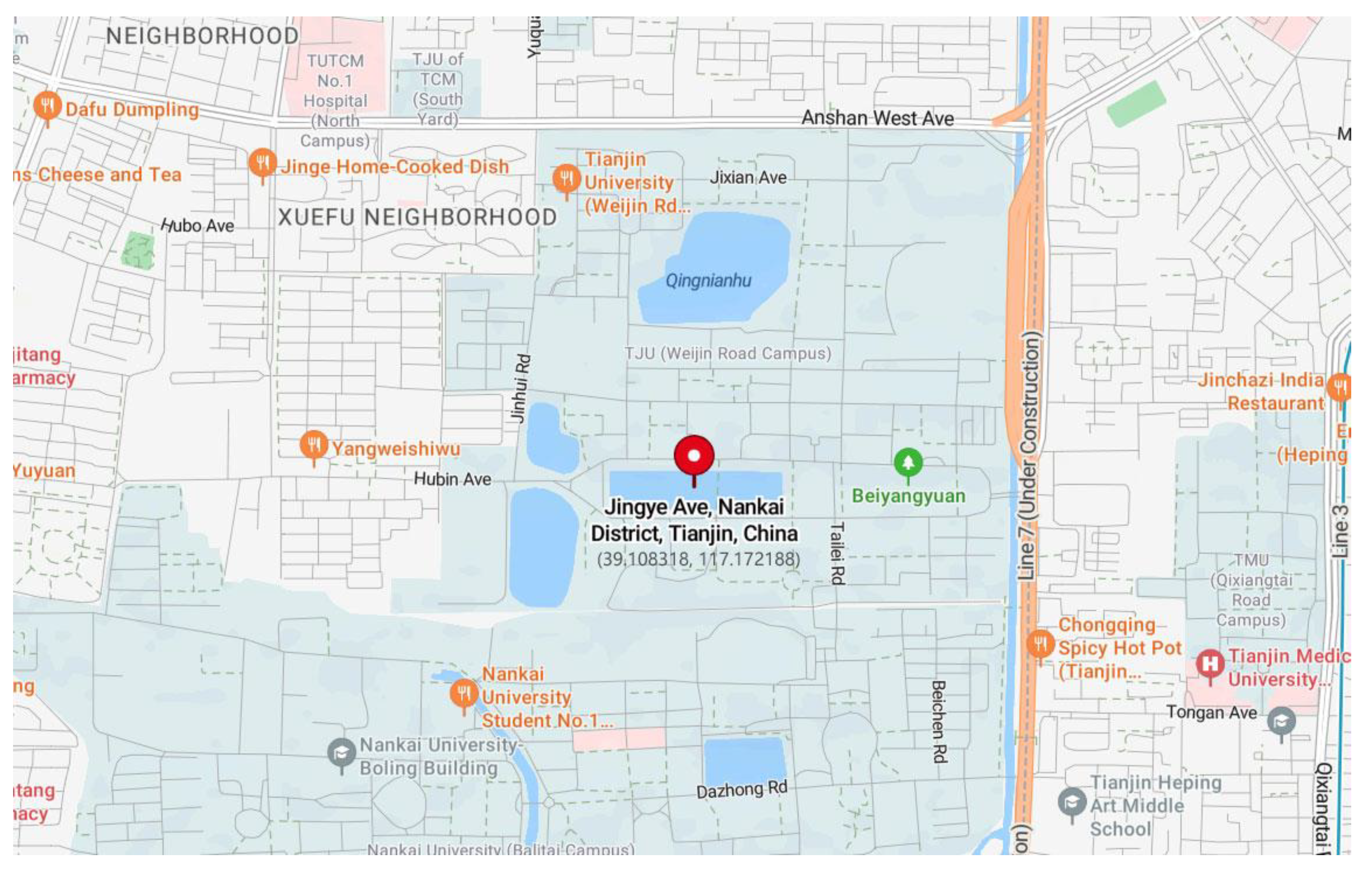
Figure 2.
Diagram of spectrum capturing and analysis of oil spill in water.
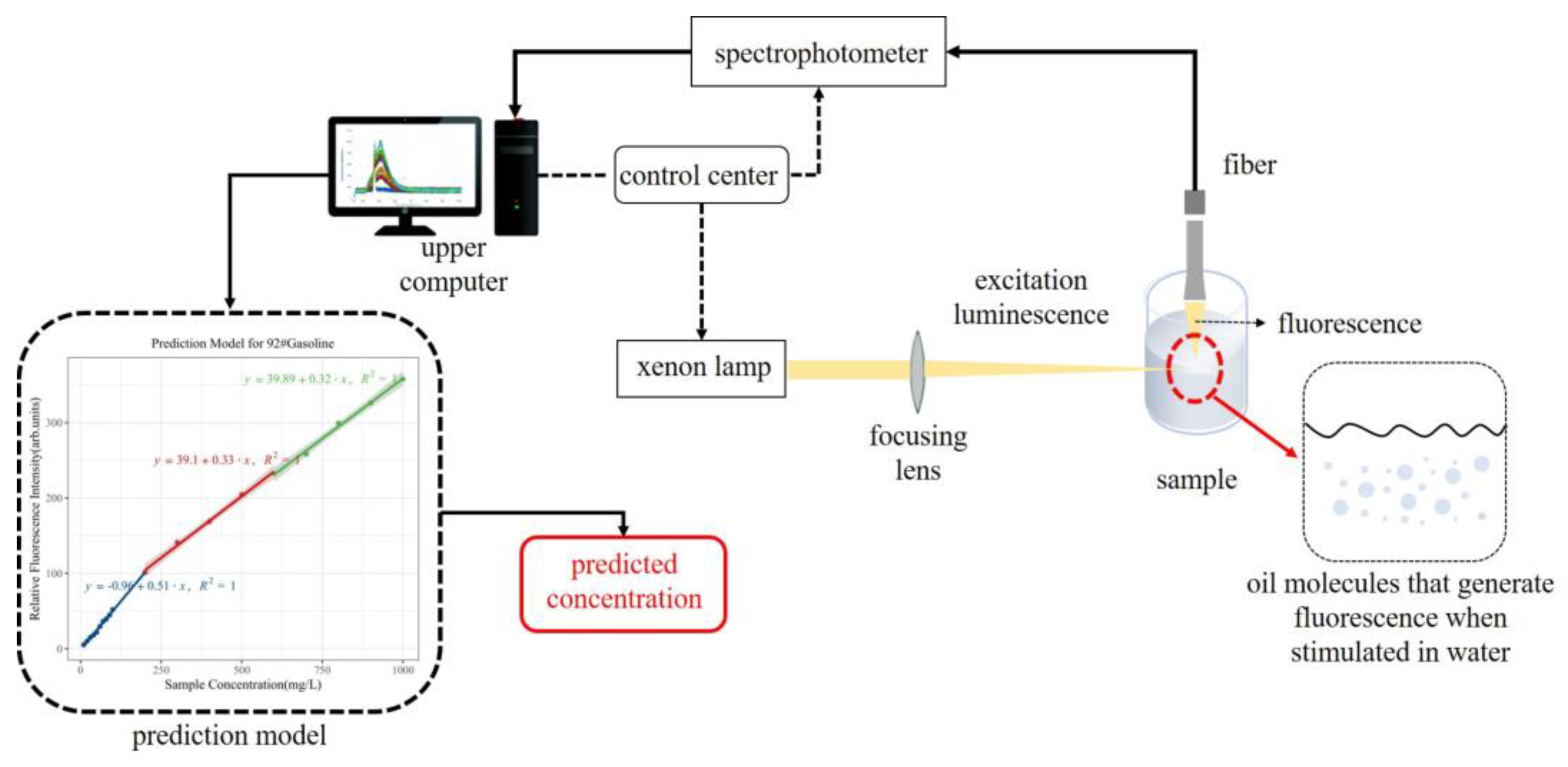
Figure 3.
RANSAC algorithm flowchart [27].
Figure 3.
RANSAC algorithm flowchart [27].
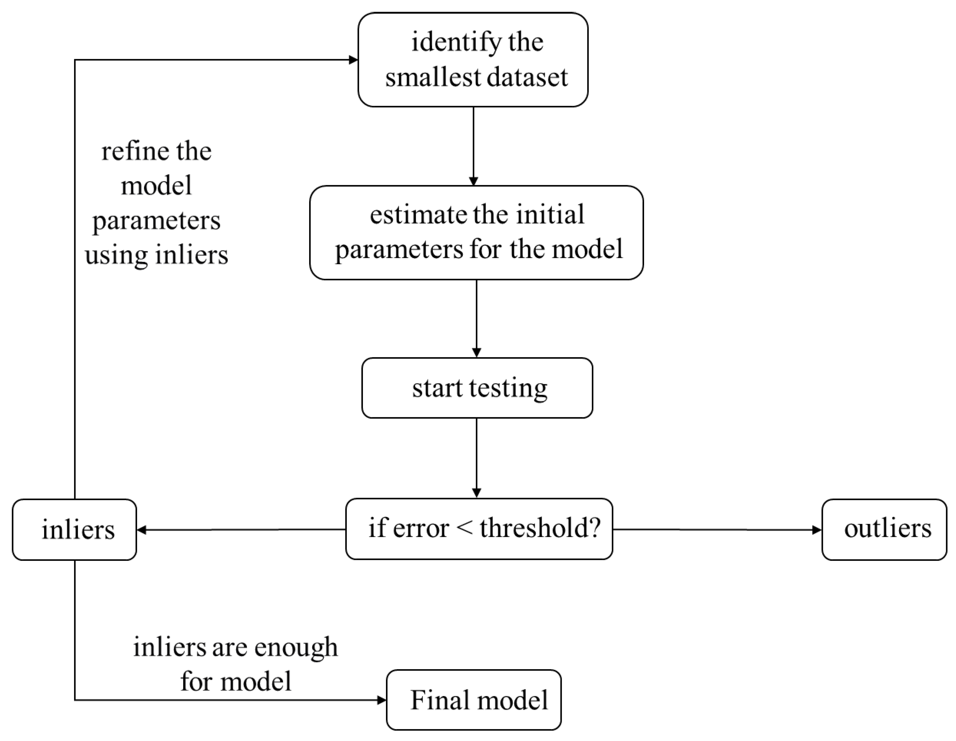
Figure 4.
Raw fluorescence spectra of different concentration samples of different oils. (a) 92# Gasoline; (b) Mobil Motor Oil 20w-40; (c) Shell Oil 10w-40; (d) Soybean Oil.
Figure 4.
Raw fluorescence spectra of different concentration samples of different oils. (a) 92# Gasoline; (b) Mobil Motor Oil 20w-40; (c) Shell Oil 10w-40; (d) Soybean Oil.
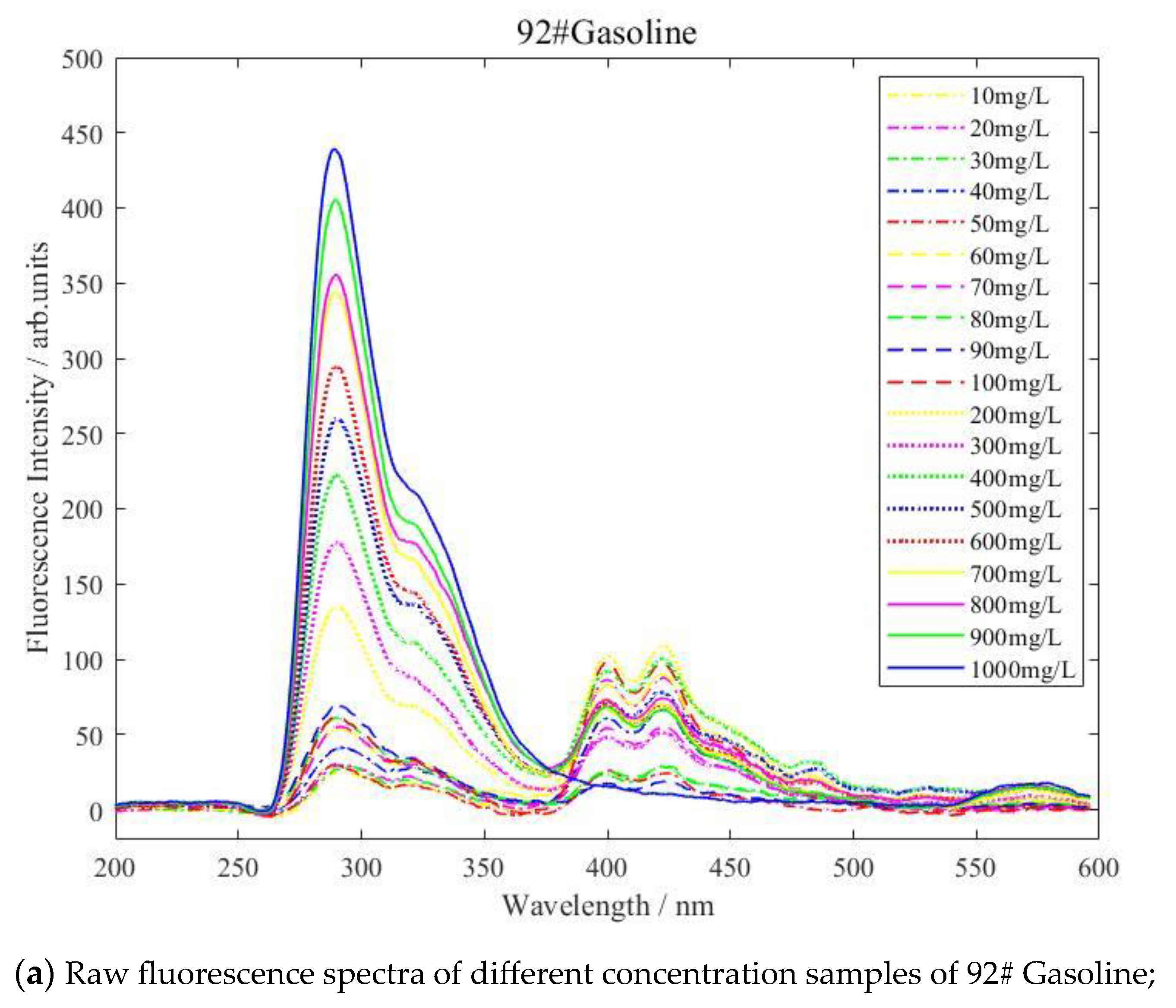
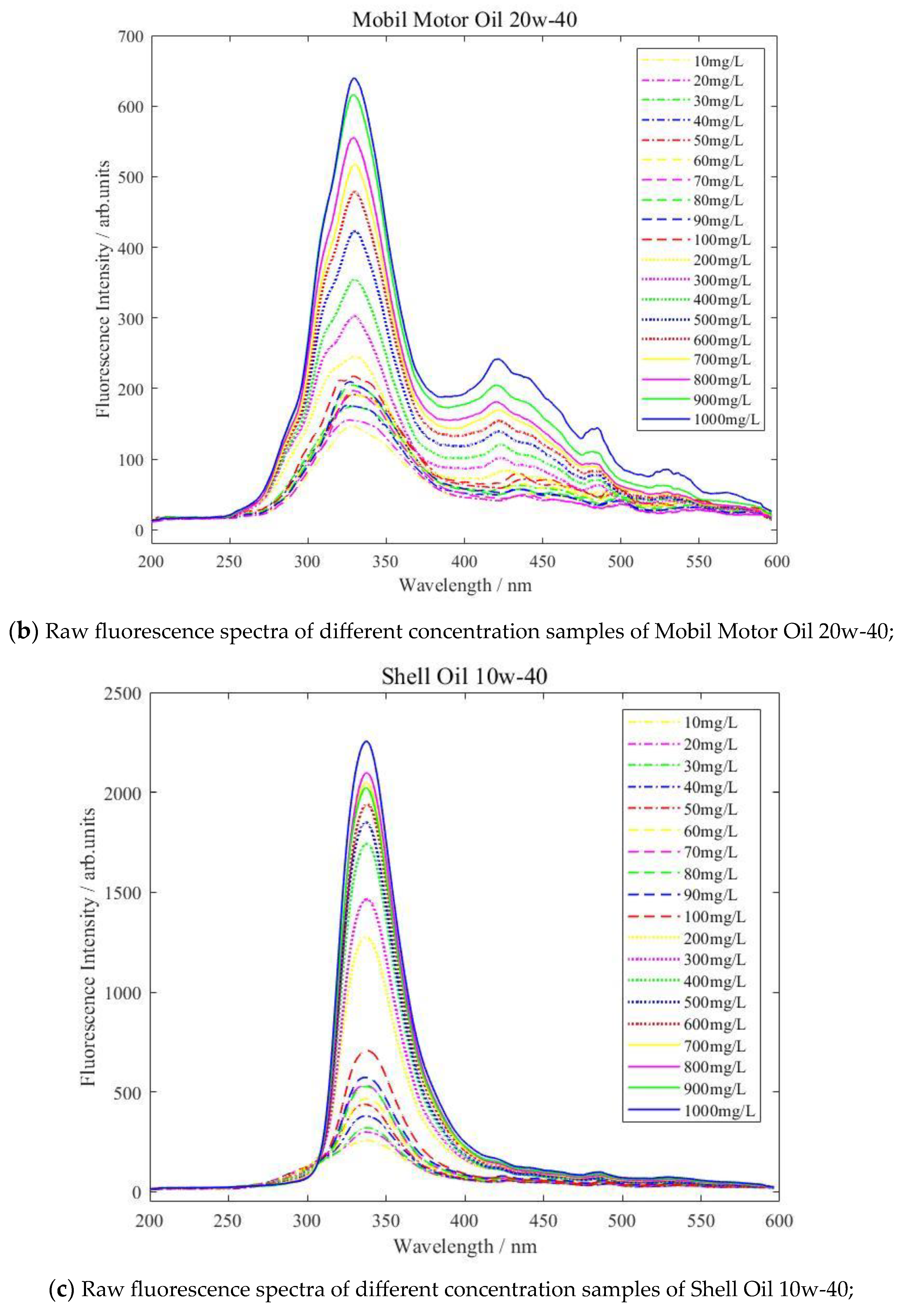
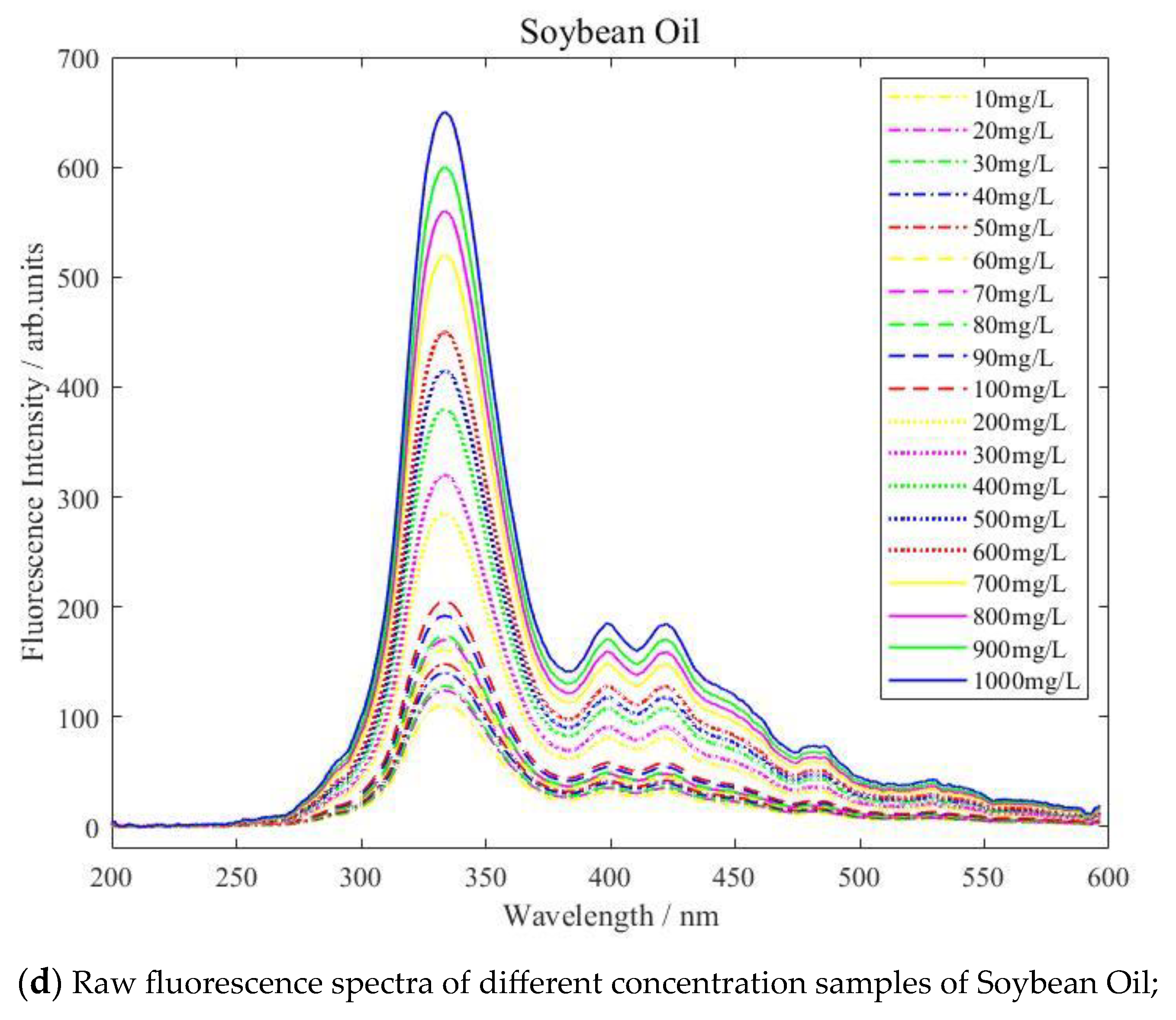
Figure 5.
Fluorescence spectra of 1000 mg/L for different oils. (a) Raw spectrogram; (b) normalized spectrogram.
Figure 5.
Fluorescence spectra of 1000 mg/L for different oils. (a) Raw spectrogram; (b) normalized spectrogram.
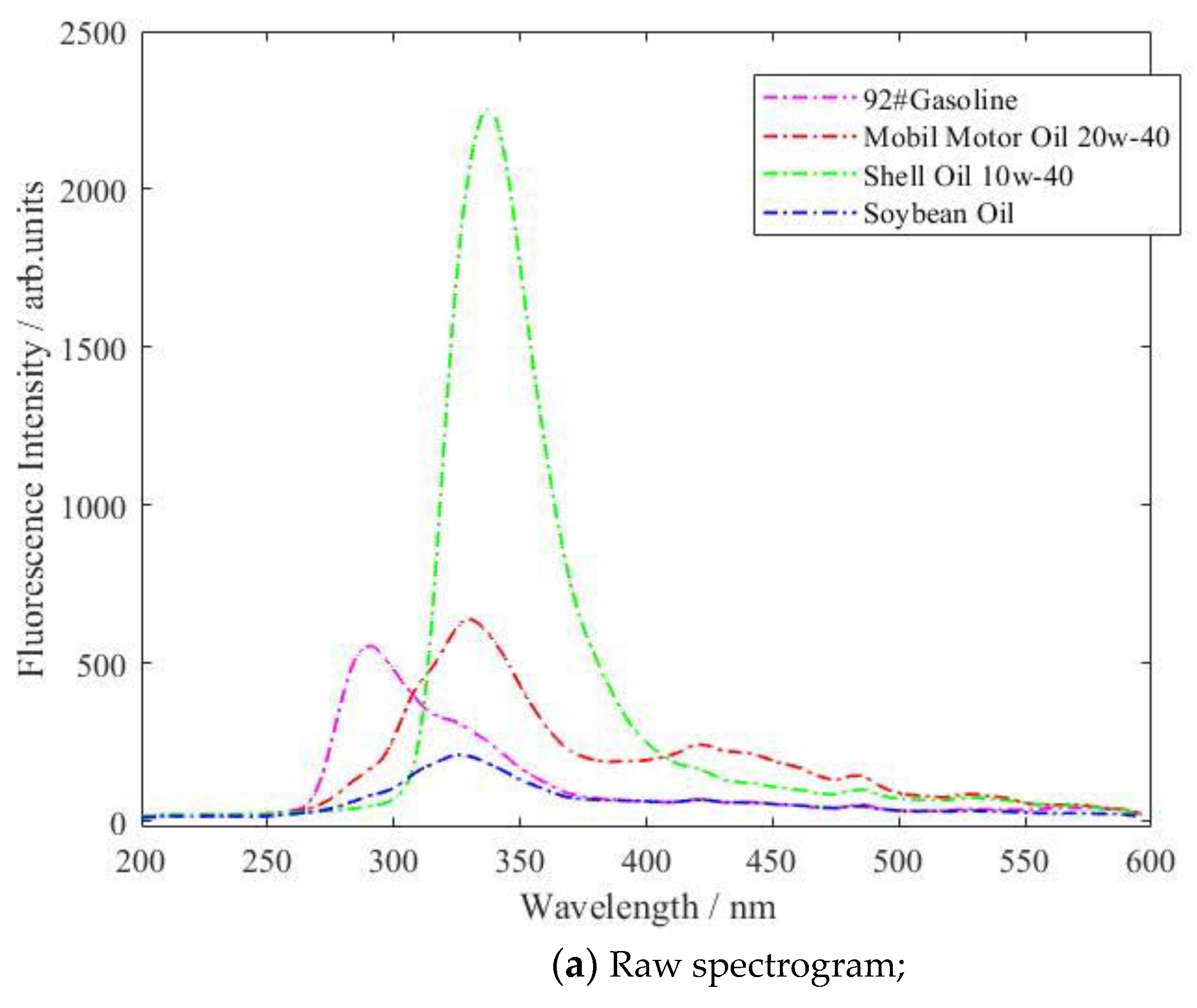
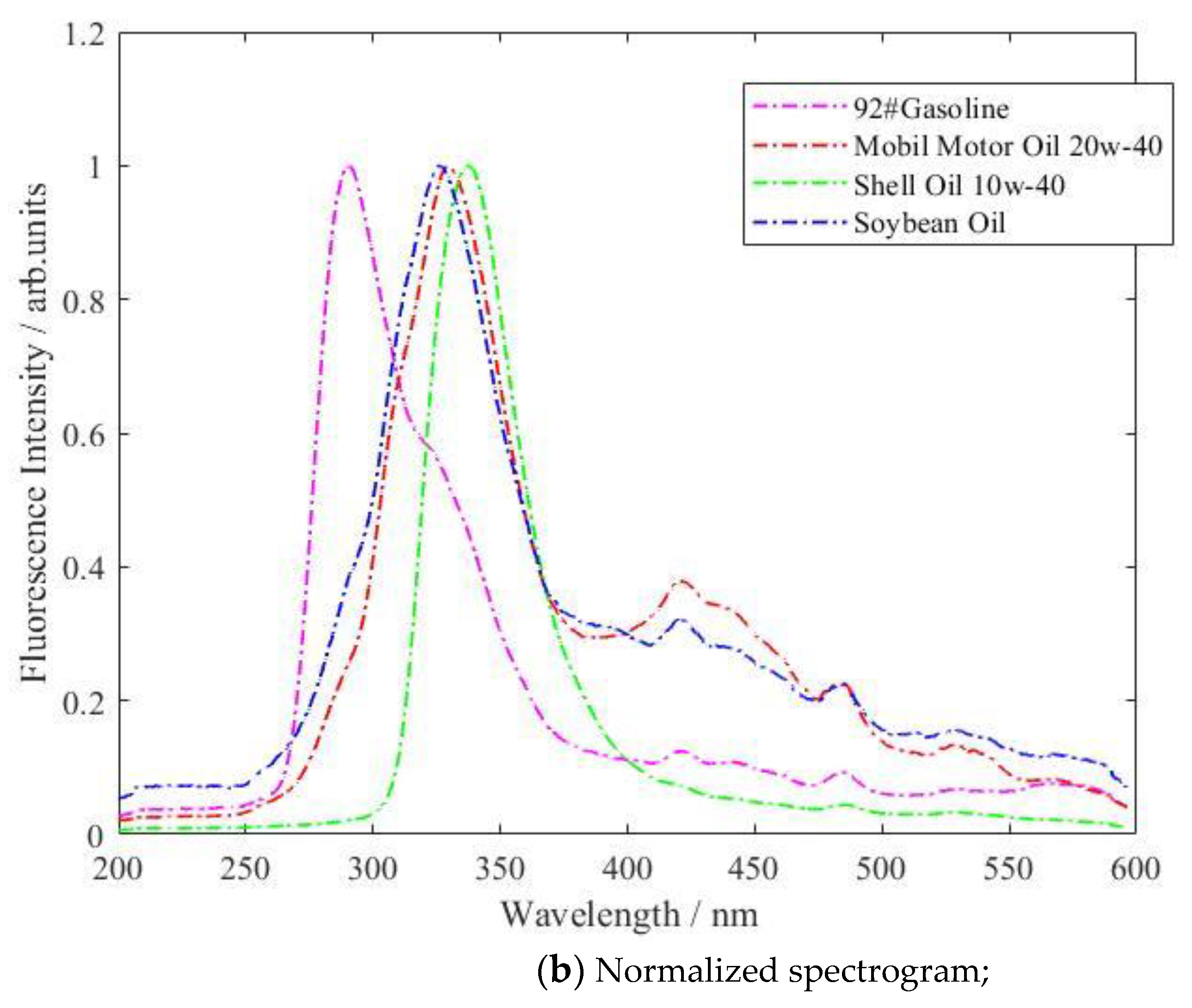
Figure 6.
Concentration prediction model for 92# gasoline based on induced fluorescence spectroscopy and RANSAC segmentation algorithm.
Figure 6.
Concentration prediction model for 92# gasoline based on induced fluorescence spectroscopy and RANSAC segmentation algorithm.
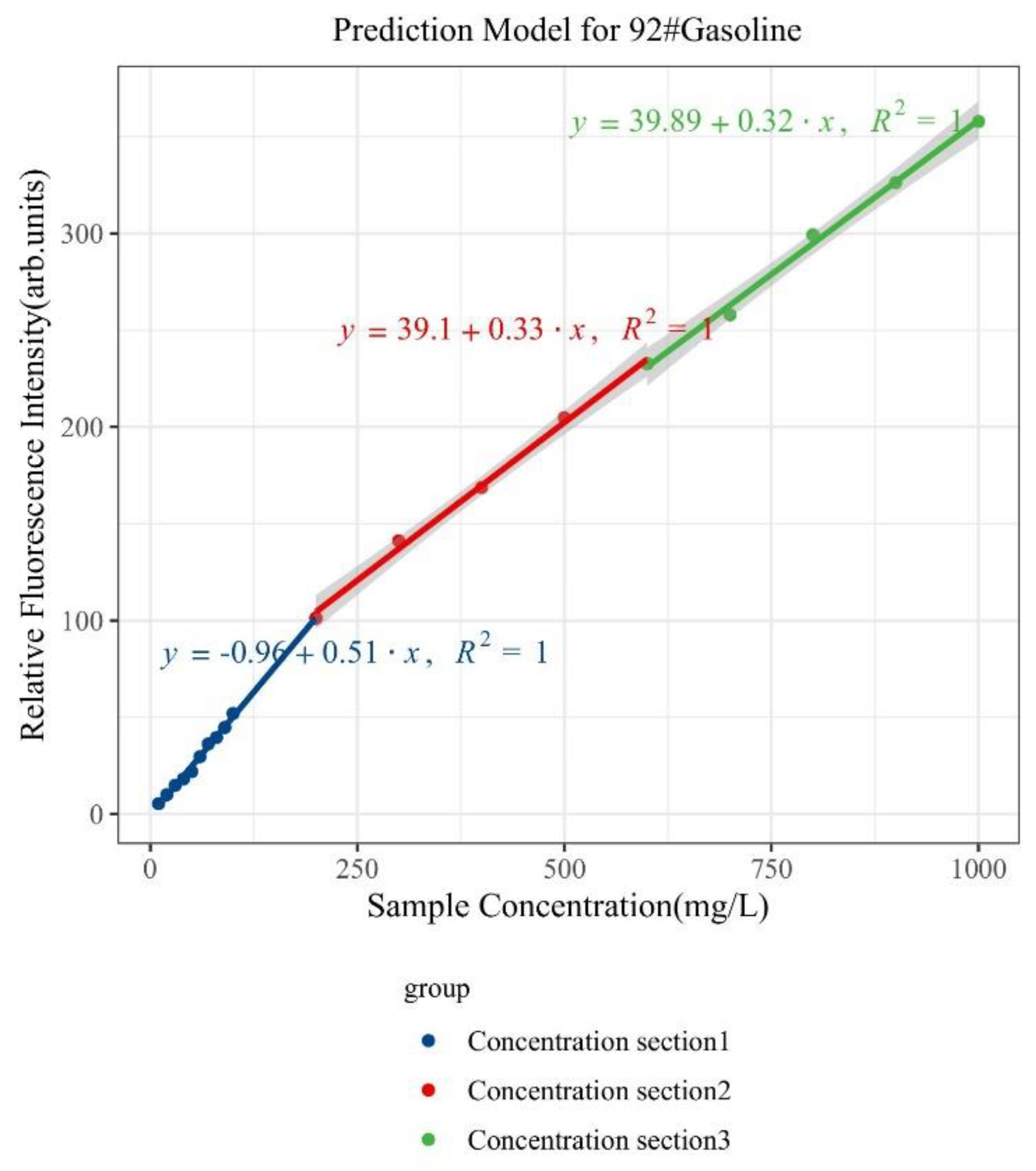
Figure 7.
Concentration prediction model for Mobil Motor Oil 20w-40 based on induced fluorescence spectroscopy and RANSAC segmentation algorithm.
Figure 7.
Concentration prediction model for Mobil Motor Oil 20w-40 based on induced fluorescence spectroscopy and RANSAC segmentation algorithm.
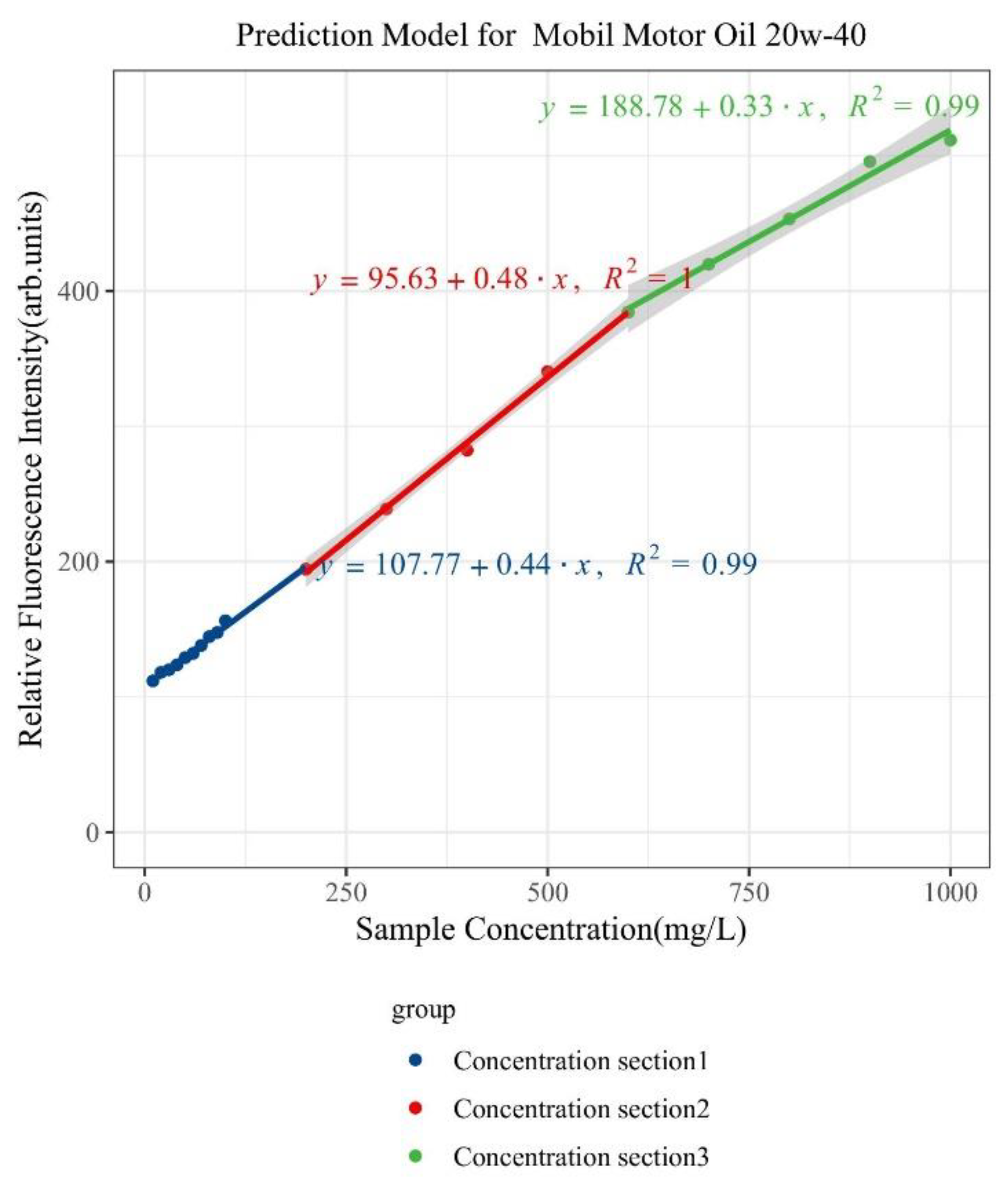
Figure 8.
Concentration prediction model for Shell Oil 10w-40 based on induced fluorescence spectroscopy and RANSAC segmentation algorithm.
Figure 8.
Concentration prediction model for Shell Oil 10w-40 based on induced fluorescence spectroscopy and RANSAC segmentation algorithm.

Figure 9.
Concentration prediction model for Soybean Oil based on induced fluorescence spectroscopy and RANSAC segmentation algorithm.
Figure 9.
Concentration prediction model for Soybean Oil based on induced fluorescence spectroscopy and RANSAC segmentation algorithm.
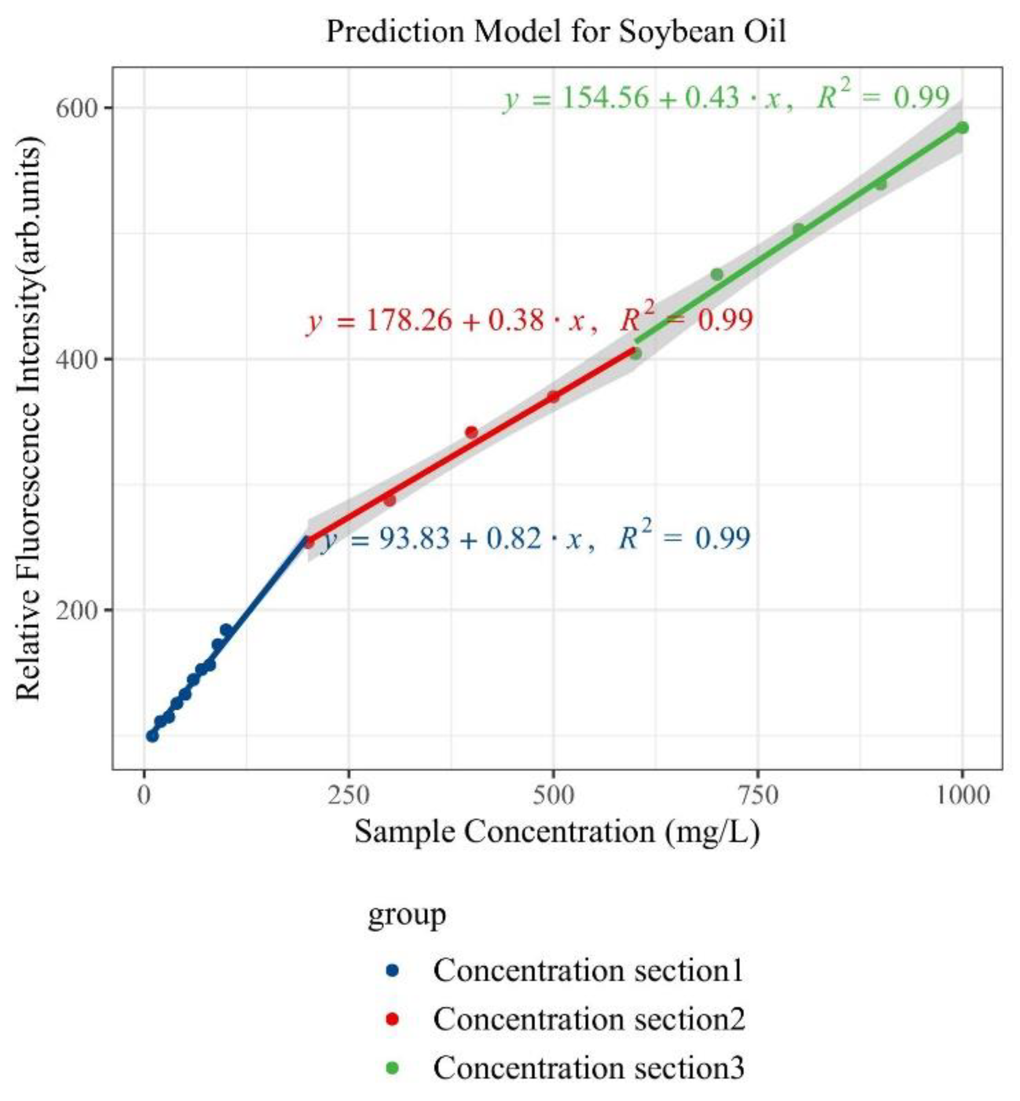
Figure 10.
Analysis of the prediction model for the high concentration of 100~1000 mg/L.

Table 1.
Experimental sample dataset.
| Type of Oil | Detection Concentration (mg/L) | Number of Data Samples |
|---|---|---|
| 92# Gasoline | 0, 10, 20, 30, 40, 50, 60, 70, 80, 90, 100, 200, 300, 400, 500, 600, 700, 800, 900, 1000 | 200 |
| Mobil Motor Oil 20w-40 | 0, 10, 20, 30, 40, 50, 60, 70, 80, 90, 100, 200, 300, 400, 500, 600, 700, 800, 900, 1000 | 200 |
| Shell Oil 10W-40 | 0, 10, 20, 30, 40, 50, 60, 70, 80, 90, 100, 200, 300, 400, 500, 600, 700, 800, 900, 1000 | 200 |
| Soybean Oil | 0, 10, 20, 30, 40, 50, 60, 70, 80, 90, 100, 200, 300, 400, 500, 600, 700, 800, 900, 1000 | 200 |
Table 2.
Detection limits for four types of oil pollutants.
| Type of Oil | Concentration | Linear Regression | Correlation Coefficient r | LOD (mg/L) |
|---|---|---|---|---|
| 92# Gasoline | 0~1000 | Y = 0.51x − 0.96 | >0.99 | 0.8 |
| Mobil Motor Oil 20w-40 | 0~1000 | Y = 0.44x + 107.77 | 0.99 | 0.9 |
| Shell Oil 10W-40 | 0~1000 | Y = 5.64x + 118.85 | 0.99 | 0.07 |
| Soybean Oil | 0~1000 | Y = 0.82x + 93.83 | 0.99 | 0.5 |
Table 3.
Oil concentration detections and actual concentration values.
| Type of Oil | Add Concentration (mg/L) | Predict Concentration (mg/L) |
|---|---|---|
| 92# Gasoline | 90 | 90.3509 |
| 400 | 399.5246 | |
| 600 | 597.7125 | |
| 900 | 902.4779 | |
| 1000 | 1004.0943 | |
| Mobil Motor Oil 20w-40 | 10 | 9.1160 |
| 300 | 297.8706 | |
| 600 | 602.7507 | |
| 700 | 700.8044 | |
| 800 | 804.1076 | |
| Shell Oil 10w-40 | 90 | 90.7007 |
| 100 | 102.9365 | |
| 200 | 196.2613 | |
| 400 | 404.0503 | |
| 800 | 798.5954 | |
| Soybean Oil | 40 | 40.3556 |
| 200 | 203.1754 | |
| 500 | 504.1037 | |
| 900 | 899.1573 | |
| 1000 | 1003.1176 |
Disclaimer/Publisher’s Note: The statements, opinions and data contained in all publications are solely those of the individual author(s) and contributor(s) and not of MDPI and/or the editor(s). MDPI and/or the editor(s) disclaim responsibility for any injury to people or property resulting from any ideas, methods, instructions or products referred to in the content. |
© 2024 by the authors. Licensee MDPI, Basel, Switzerland. This article is an open access article distributed under the terms and conditions of the Creative Commons Attribution (CC BY) license (https://creativecommons.org/licenses/by/4.0/).
Share and Cite
MDPI and ACS Style
Wu, H.; Wang, Z.; Zhao, Y. Rapid Investigation of Oil Pollution in Water-Combined Induced Fluorescence and Random Sample Consensus Algorithm. Sustainability 2024, 16, 3930. https://doi.org/10.3390/su16103930
AMA Style
Wu H, Wang Z, Zhao Y. Rapid Investigation of Oil Pollution in Water-Combined Induced Fluorescence and Random Sample Consensus Algorithm. Sustainability. 2024; 16(10):3930. https://doi.org/10.3390/su16103930
Chicago/Turabian StyleWu, Hui, Ziyi Wang, and Youquan Zhao. 2024. "Rapid Investigation of Oil Pollution in Water-Combined Induced Fluorescence and Random Sample Consensus Algorithm" Sustainability 16, no. 10: 3930. https://doi.org/10.3390/su16103930
Note that from the first issue of 2016, this journal uses article numbers instead of page numbers. See further details here.