Article

Numerical and Experimental Analysis of a Low-GWP Heat Pump Coupled to Electrical and Thermal Energy Storage to Increase the Share of Renewables across Europe

by
Omais Abdur Rehman
1,2,
Valeria Palomba
1,
Andrea Frazzica
1,*,
Antonios Charalampidis
3,
Sotirios Karellas
3 and
Luisa F. Cabeza
2
1
CNR Institute for Advanced Energy Technologies (ITAE), 98126 Messina, Italy
2
GREiA Research Group, Universitat de Lleida, 25001 Lleida, Spain
3
Laboratory of Steam Boilers and Thermal Plants, National Technical University of Athens, 15780 Athens, Greece
*
Author to whom correspondence should be addressed.
Sustainability 2023, 15(6), 4973; https://doi.org/10.3390/su15064973
Submission received: 25 January 2023 / Revised: 6 March 2023 / Accepted: 8 March 2023 / Published: 10 March 2023

Abstract

:
In order to reduce the dependence on fossil fuels in the residential sector, low-carbon-footprint technologies such as heat pumps should be used. To fully exploit solar-assisted heat pumps, an effective control strategy is required. This study employs a low-global-warming-potential (GWP) refrigerant for a water-to-water reversible heat pump, which is assisted by a thermal energy storage tank, photovoltaic (PV) installation, and battery storage system using a dedicated control strategy. The heat pump’s operation is validated against the experimental data. Simulations are carried out for three different climates to analyze the performance of reversible heat pumps across Europe. The reversible heat pump fully meets the summer cooling demand in all three climates, while the heating demand is covered with the help of a backup source. An economic analysis is carried out for three different PV sizes and the results are compared with the reference energy systems. The inclusion of a battery storage system results in high payback times but increases overall flexibility and self-sufficiency.

1. Introduction

The current environmental crisis is driving the fast evolution of low-carbon-footprint technologies and related policies. Research in recent years has made it clear that in order to reduce our carbon footprint, our attention needs to be diverted toward residential and commercial buildings, which account for 40% of the total primary energy consumption in the European Union (EU) [1]. Heating, ventilation, and air conditioning (HVAC) account for 76% of this primary energy consumption [2]. It is also common knowledge that the primary energy consumption of existing buildings needs to be reduced, which is possible in two ways. One way is to increase the energy performance of buildings by improving the insulation of outer walls and windows; the other way is to replace the existing heat generators, which run on fossil fuels [3]. In the latter case, major energy savings can also be made, along with the co-benefit of reduction in carbon emissions since the increase in fuel prices over the last few years or so.
Therefore, much of the research in recent years focused on how to reduce energy consumption and CO2 emissions, while also keeping HVAC technology reliable for maintaining thermal comfort in the buildings. Moreover, the heating and cooling sector needs to be electrified in order to reduce carbon emissions. Heat-pump technology can be used to address this challenge since it is a highly efficient system with a low carbon footprint compared to other contemporary heating and cooling technologies [4].
Another aspect to be considered is that solely reducing the energy consumption of HVAC technologies is not enough. The new concept of nearly zero-energy buildings (nZEB) has seen a prominent rise in recent years [5]. The exact definition of such a building does not exist in the literature; the main concept is that an nZEB building must be able to meet its energy demand by using the available efficient technologies, along with generating enough thermal and electrical energy with the help of renewable energy sources (RES) so that the overall energy balance is close to zero [6]. A true nZEB building is not possible because of various technical and economic challenges but efforts are underway to construct new buildings or renovate the old ones in such a way as to accommodate the use of efficient HVAC technologies, along with RES, to reduce the carbon footprint [7,8].
Such buildings need sophisticated controls to regulate the working of these systems and to experience the full benefit of heat pumps and variable RES [3].
A number of studies have been conducted on this topic. Zanetti et al. [9] studied the energy cost savings made when using a solar-assisted heating system. An optimal rule-based control strategy, developed in MATLAB, was applied to see whether there was any change in the results for cost savings. A radiant floor heating system was considered, with an air-source HP and a gas boiler as heating sources, along with a water tank as thermal energy storage. A battery energy-storage system was not considered in this study. It was concluded that a heating system with an optimal control strategy resulted in a 20% energy consumption cost and increased the PV self-consumption by up to 30% compared to a state-of-the-art rule-based control strategy. Another study published by Li Gang [10] investigated a configuration consisting of air-source HP with a gas-fired water heater with a new control strategy to assess the cost benefits. The applied control strategy led to ~10% to ~60% of economic benefits within a temperature range of −12 to 20 °C for space-heating applications in China. Moreover, a high fuel price ratio resulted in a lower ratio of heat supplied by HP. A lower fuel price ratio helped for achieving higher economic savings. Thieblemont et al. [11] carried out a review of control strategies for buildings with an energy storage system and concluded that in order to have a high-performance system while having RES incorporated in buildings, along with a thermal energy storage unit, a proper control system is needed to achieve the maximum benefit. Bagarella et al. [12] developed a TRNSYS model for a hybrid HP and carried out simulations in two different climates, using a control strategy employing an HP in either parallel mode or individual mode. It was concluded that a hybrid system can result in savings of up to 5% in a cold–humid climate, with up to 8% of savings in a mild–dry climate.
Chen et al. [13] developed a model for a hybrid solar-geothermal system, including solar collectors and a ground-source HP, in a rural area near Shanghai, China. The model was implemented using the open-source “Buildings” library in Dymola. The seasonal coefficient of performance (SCOP) with and without solar thermal collectors was 4.2 and 3.5, respectively. When HP worked alongside renewable energy in combination, the self-sufficiency index (SSI) reached around 45%. It is worth noticing that the developed model did not include any battery energy storage system or solar PV system.
Beccali et al. [14] investigated suitable renewable methods to supply thermal comfort to a hotel on a Mediterranean island (Lampedusa) during the summer season. The hotel had air-to-water heat pumps for providing thermal comfort as well as hot water. The use of solar collectors resulted in a 55% energy reduction in air conditioning and the grid’s peak load was reduced. Eslami et al. [15] studied a hybrid solar system to provide electricity, domestic hot water, and drinking water in a park. The simulation results were validated with experiments and the results confirmed the feasibility of the system. Payback times were calculated for a solar water heater, desalination system, and PV, which were 4.4, 1.6, and 2.3 years, respectively. Ciriminna et al. [16] identified several major barriers to the adoption of renewable technologies in a Mediterranean climate, mainly referring to the regional policies and landscape of the island. The subsidy provided for fossil fuel consumption is also a major hindrance in the rise of RES use. As the prices of PV and wind have now been reduced to a great extent, there is an increased interest in installing PV and wind technologies at a local level in the Mediterranean islands.
Calise et al. [17] proposed a system consisting of a solar-assisted water-to-water reversible heat pump. The main aim of the study was to minimize the payback time of the energy system. For this purpose, a dynamic simulation model was developed in TRNSYS. To reduce the payback time, the main set of control parameters was obtained via sensitivity analysis. A payback time of 5.36 years was found for a one-story building in Naples. If the country or the wider region has a capital incentive policy of 30%, the payback time reduces by 2.33 years. This study also highlights the importance of incentive policies in order to encourage the installation of low-carbon HVAC technologies. In another study, Calise et al. [18] analyzed micro wind turbines and integrated PV panels at the building level, incorporating high-efficiency heat pumps for space cooling and heating, along with domestic hot water. The authors concluded that 61% of the total electricity demand was covered by renewables. The incorporation of heat pumps for space heating/cooling and domestic hot water led to a reduction in primary energy demand by 27%. Roselli et al. [19] investigated the integration of a PV system with a heat pump and electrical storage for an office in Southern Italy. The energy and environmental performance of the proposed system was evaluated and a reduction in carbon dioxide emissions by 93% was reported, along with high energy savings. Ma et al. [20] performed a thermo-economic analysis of a reversible HP-organic Rankine cycle power system with electrical storage capacity; they optimized storage temperatures using the TOPSIS method. The levelized cost of the system was calculated and came out at USD 0.36/kWh. Cirone et al. [21] performed a techno-economic analysis of an energy community, based on PV and electric storage systems in Southern Italy. Photovoltaic generators and electrical storage cooperate to provide energy to heat pump systems to maximize self-consumption. Their study is based on dynamic simulations performed in TRNSYS. The results showed an 80% reduction in CO2 emissions.

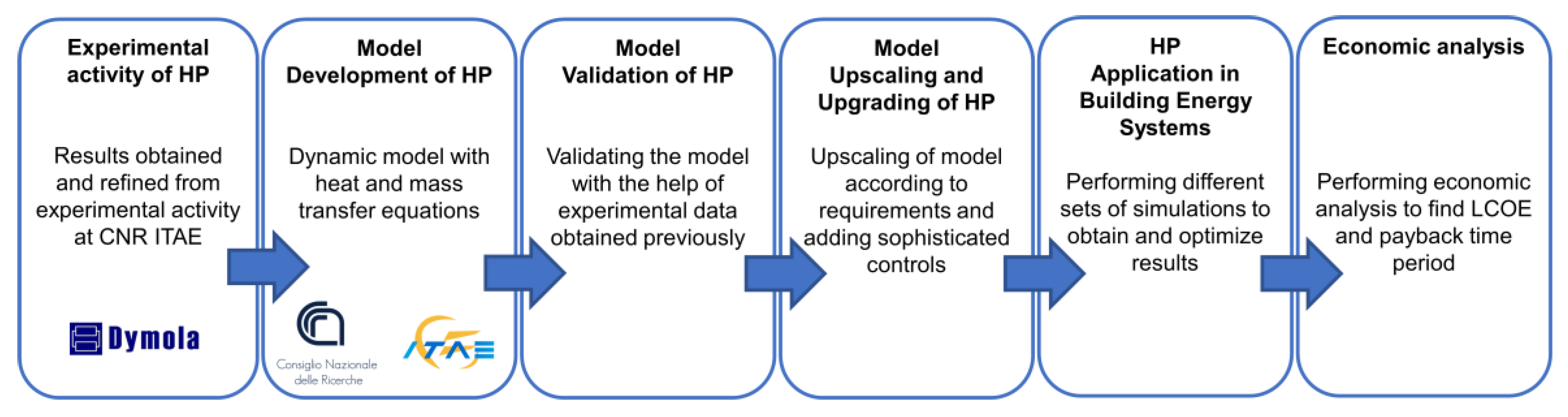
Paper Positioning and Methodology

From the literature analysis reported above, it is clear that hybrid systems are the preferred solution in terms of the reduction of emissions in the atmosphere and the increase in energy efficiency. At the same time, an aspect that is gaining importance in the present period is the need for the buildings to be as self-sufficient as possible from the energy point of view, thus reducing the energy that is draining from the grid. Another factor that can be deduced from the literature is that there is little to no data available about the performance of HP with the refrigerant R1234Ze(E). Most of the studies have been carried out with commercial refrigerants, such as R134a, R407c, and R410a. This is one of the first studies that employ the low-GWP refrigerant R1234Ze(E) in a reversible heat pump at a residential level. In this study, a hybrid system for residential applications is evaluated from the energy and economic points of view. The system includes a solar-assisted 10 kW reversible water-to-water heat pump (HP) and thermal and electric storage. The main component of the system, i.e., the heat pump model, is based on a prototype of a small-size heat pump, suitable for single-family houses, that employs the low global-warming-potential (GWP) refrigerant R1234Ze(E), the performance of which was experimentally evaluated through a dedicated activity. The cities selected for simulations were Athens, Marseille, and Stuttgart, which have different climate types, in order to give a European perspective and systematic analysis. These cities have Mediterranean, hot semi-arid, and humid continental climates, respectively [20].
Moreover, previous studies lacked the simultaneous presence of thermal energy storage, electrical storage, and solar assistance. Even if such studies exist, they are lacking in details regarding the economic analysis. This study employs a new refrigerant and includes solar assistance, as well as thermal and electrical storage. Moreover, the thermal components used for modeling were validated with experimental data. The data for the batteries used for electrical storage were also drawn from experimental activities performed at CNR ITAE. Lastly, an economic analysis based on three different European climates is presented, which, along with the previously mentioned novel elements, makes this study unique among previous studies. The economic analysis also provides a comparison with a reference heating and cooling system. Most of the previous studies mainly focus on a specific climate for analyzing the behavior of a heat pump, while this study analyzes its behavior in three different climates.
Another point worth mentioning is that in addition to the energy analysis, an economic analysis in comparison with contemporary technologies is carried out. This is performed by considering, on the one hand, the energy exchange of the house with the grid and, on the other hand, by systematically analyzing the subsidies, tax regulations, and incentives given for installing HP or RES technologies, with a special focus on Greece, Germany, and France, the countries considered for the simulations. Discounted payback time, along with the levelized cost of energy (LCOE), are calculated and the results are discussed accordingly.
The methodology followed for the study is presented in Figure 1: starting from the experimental activity on the low-GWP heat pump, a model was developed in the Modelica language and in a Dymola environment. After validation, the application of the heat pump within a complete residential building energy system was considered and energy and economic analysis were carried out.

2. Experimental Activity

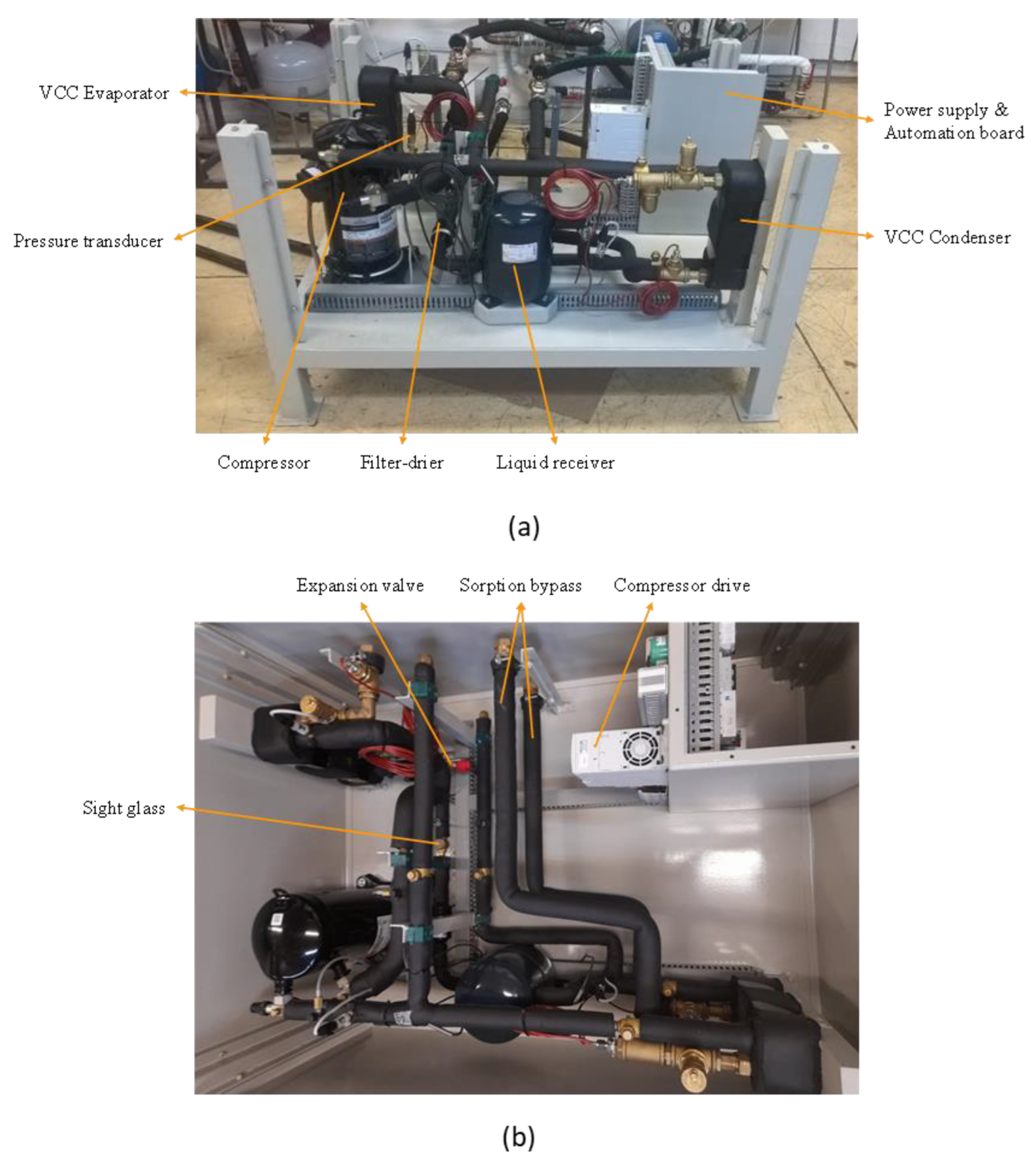
2.1. The Investigated System

As highlighted in the introduction, the decarbonization of the heating and cooling sector will require low-GWP heat pumps. Accordingly, a prototype was built to be operated as a small-size reversible heat pump that is suitable for residential applications and employs a low-GWP refrigerant, i.e., R1234ze(E). The main features of the heat pump are listed in Table 1. The specific selection of the refrigerant, among the various available options, was carried out mostly for two reasons: first, R1234ze(E) can be used as a drop-in replacement for R134a, which is one of the most commonly employed refrigerants in the residential and commercial sectors; second, this specific refrigerant can also be used for high-temperature heat pumps and organic Rankine cycles (ORC,) which would allow the further extending of the potentialities of the heat pump (e.g., as a reversible heat pump/ORC) in the future.
A detailed view of the reversible heat pump is given in Figure 2 below, wherein all the main components are highlighted. Figure 2a,b refers to the main components of reversible HP through different angles. The main peculiarity of the reversible heat pump is the use of this kind of refrigerant for a domestic-sized system. The refrigerant used has a GWP value of 7, while traditional refrigerants such as R134a, R407c, and R410a have GWP values of 1430 [22], 1774 [22], and 2088 [22,23], respectively. Compared to other refrigerants that are becoming increasingly popular in domestic applications as low-GWP alternatives (most notably, R290 and R600a), R1234ze(E) is classified as an A2L refrigerant, i.e., it has low flammability, whereas R290 and R600a are in class A3 (highly flammable refrigerants). This increases the intrinsic safety of the heat pump. To the authors’ best knowledge, however, there are no commercial systems employing such a refrigerant in small-scale reversible heat pumps.
A schematic diagram of the reversible HP, along with its sensors, is given below in Figure 3. The heat pump prototype was equipped with all the relevant sensors for monitoring and performance evaluation. Specifically, Pt100 temperature sensors were installed directly on the inlet/outlet of the HTF circuit and at the inlet/outlet of the evaporator and condenser refrigerant circuit. In addition, 3 piezoelectric pressure sensors were installed at the inlet/outlet of the condenser and at the outlet of the evaporator.

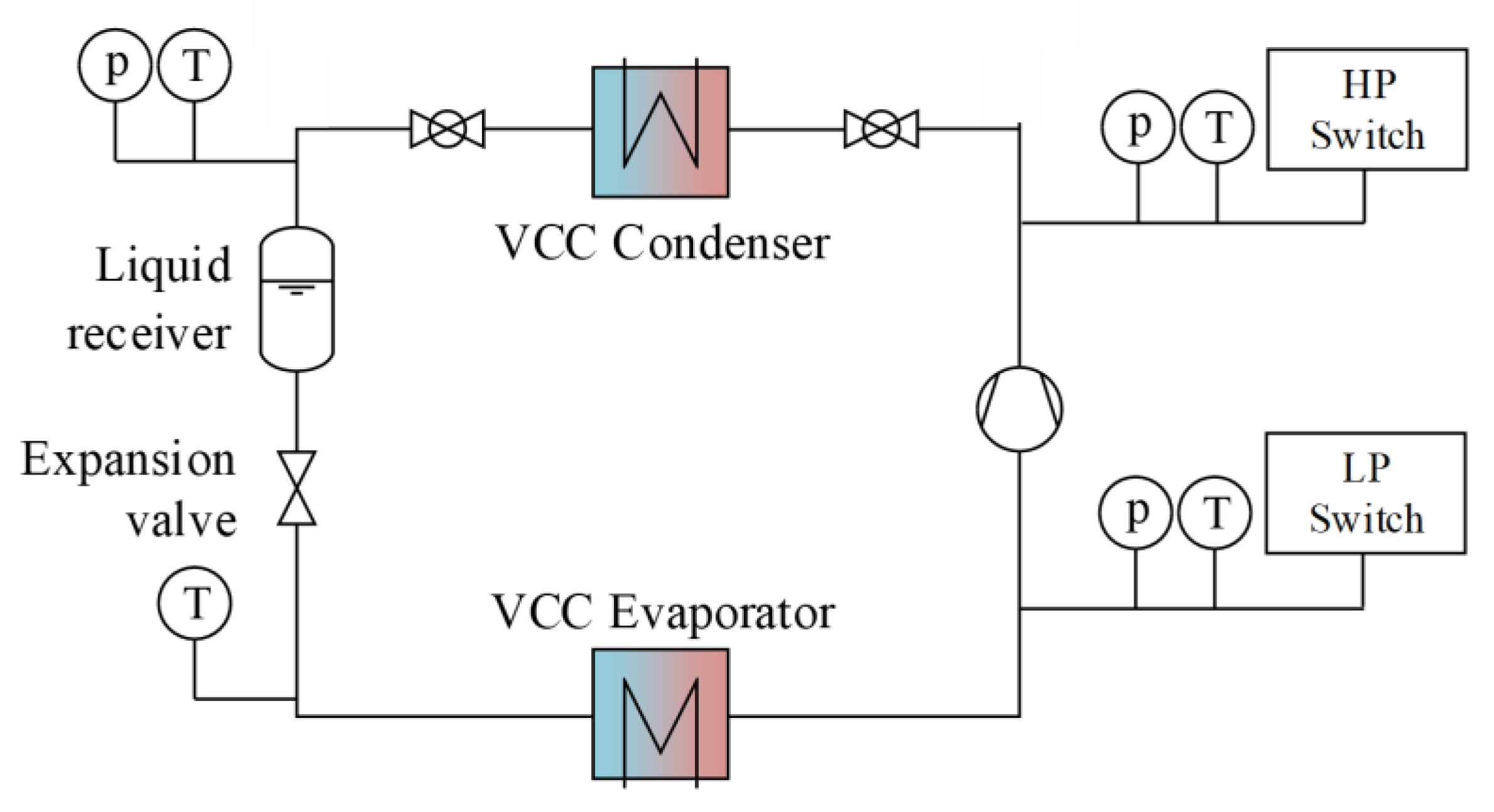
2.2. Description of Testing Rig

All tests were performed on a testing rig that was available in CNR ITAE in Messina, as described in [24,25]. The testing activity was focused on an evaluation of the performance of the reversible heat pump when in cooling mode (i.e., under summer conditions) since the target application is for use in climates with predominantly cooling demands. The system cooling capacity, along with the energy efficiency ratio (EER), was evaluated at different operating temperatures and compressor speeds. The testing rig was specifically designed for testing thermal and hybrid components.
The reversible heat pump was also connected to the same control program for the recording of the values of the sensors that had been installed and are discussed in the previous section. Similarly, the compressor speed can also be controlled via this monitoring setup. The compressor is run by means of a PID control, with auto-tune features realized directly on the control software, using as a reference value the set-point temperature for the outlet of the HTF circuit of the evaporator.

2.3. Testing Procedure

A typical test is run according to the following steps:
  • All electrical circuits are turned on. Pumps for the circulation of heat transfer fluid (HTF) in the condenser and evaporator reach the desired speeds, while the desired temperature for the condenser and evaporator inlet is set.
  • The compressor is turned on and its speed is controlled from a control panel realized in LabVIEW. Superheating is set to 6 K.
  • The test is started with a data acquisition rate of 1 s. Once a steady state is achieved, at least 1000 s of acquisition time for each condition is recorded. All values from the sensors are stored in a Notepad file.

2.4. Data Analysis

Experiments were performed for operating temperatures (at the HTF condenser inlet) of 26 °C, 29 °C, 32 °C, 35 °C, and 40 °C, respectively, while running the compressor at 1500, 2100, 2400, and 2800 rpm. The selected evaporator temperatures at the inlet/outlet are 12 and 7 °C, which corresponds to a typical domestic application [26]. Table 2, presented below, shows the scheme of performed tests.
In order to assess the performance of the HP, several significant parameters were calculated with the help of measured data. These parameters include the logarithmic mean temperature difference (LMTD) at the condenser and evaporator side, UA (the product of the overall heat transfer coefficient and surface area) for the condenser and evaporator, the energy efficiency ratio (EER), and the pressure ratio. LMTD is defined as a logarithmic average of the temperature difference between hot and cold feeds at each end of a heat exchanger. Conversely, the UA value measures how effective a material is as an insulator. A lower UA value means lesser heat losses. The equations to find LMTD and UA for both the condenser and evaporator are given below in Equations (1)–(4).
Moreover, the energy efficiency ratio and pressure ratios were calculated according to Equations (5) and (6). The energy efficiency ratio (EER) represents the ratio of the useful effect in summer mode (i.e., the cooling power) over the electricity consumption of the compressor. It is one of the most critical parameters by which to gauge the performance of a reversible heat pump. The pressure ratio is defined as the ratio of pressures to the inlet and outlet of the compressor. Along with other parameters, this parameter was calculated so that it could be used for modeling the reversible heat pump.
L M T D c o n d   K = R e f c o n d i n H T F c o n d o u t H T F c o n d i n ln R e f c o n d i n H T F c o n d o u t H T F c o n d i n
U A c o n d e n s e r W / K = Q ˙ c o n d L M T D c o n d
L M T D e v a p K = H T F e v a p i n R e f e v a p o u t H T F e v a p o u t R e f e v a p i n   ln H T F e v a p i n R e f e v a p o u t H T F e v a p o u t R e f e v a p i n
U A e v a p o r a t o r W / K = Q ˙ e v a p L M T D e v a p
EER   kW kW = Q ˙ evap P e l c o m p
P r e s s u r e r a t i o bar bar = p comp in p comp o u t
The final results obtained from the HP testing are given in Figure 4. These figures contain a comparison of the measured parameters at different rpms. Uncertainty analysis was performed for these results, the details of which can be found in S2 of the Supplementary Materials. The uncertainty obtained for cooling power and EER is in the range of 4–5%. The x-axis contains the condenser HTF inlet temperature.
Figure 4a represents the cooling power at different rpms. It can be seen that decreasing the speed of the compressor results in lower cooling power. From Figure 4b, it is evident that the energy efficiency ratio (EER) decreases when increasing the condenser inlet temperature. The compressor needs to work at a higher pressure and speed in order to cool down the refrigerant, which requires a higher electrical input. The increase in electrical energy results in a decrease in the EER. The same trend is obtained for EER values for all revolutions per minute (rpm). The EER values obtained are in the range of 4–8. A literature search was made to compare the EER values available in the literature for water-to-water HP under similar operating conditions and in a similar power range (<20 kW heating capacity). The HPs considered in these studies also include systems currently available on the market. The system considered in this study has a better performance compared to those in the literature and on the market. The values reported for the EER for water-cooled chillers in the literature and on the market were in the range of 2.5–4.5 [27,28,29].
Figure 4c,d shows the comparison of pressure ratios at different rpms. The pressure ratio is defined as the ratio of the refrigerant pressure when leaving the compressor to the pressure of the refrigerant entering the compressor. The results show that with an increasing condenser inlet temperature while keeping the compressor speed constant, the pressure ratio increases. The reason is that because of an increase in operating temperature, the pressure ratio needs to be increased in order to meet the cooling load demand on the evaporator side.
Figure 4d shows the effect of increasing the operating temperature upon valve opening. It can be seen that with increasing condenser inlet temperatures, the valve opening reduces. An important thing to mention here is that the PI controller regulates the opening of the expansion valve and continuously receives input from the superheating sensor. Superheating is set at 6 K. As the condenser HTF temperature increases, the refrigerant temperature also increases at the condenser outlet; therefore, the expansion valve needs to regulate the refrigerant in such a way that the superheating of 6 K is achieved after the evaporator. This is due to the fact that the higher temperature of the refrigerant leads to less of an opening to the expansion valve; thus, less refrigerant is processed.
The outcomes of the experimental activity were used for the development of the heat pump model in the Modelica language for its subsequent integration into an energy system, which will be discussed in the following section.

3. Modeling Activity

The heat pump (HP) model is developed using Dymola, a commercial software that is used for the modeling and simulation of complex integrated systems [30]. One of the most useful features of Dymola is the incorporation of compatible libraries from different engineering fields, such as thermal, electrical, and mechanical fields, etc. Another useful feature of Dymola is its functional mock-up interface (FMI), which allows the built model to be transported to or integrated into a different modeling and simulation environment. All components of this software were developed in Modelica, which is an object-oriented language.
The libraries used in this study for modeling are TIL, TIL media, TIL file reader, and Photovoltaics. TIL is a Modelica library that helps to simulate transient thermal systems [31]. Control strategies can also be developed and tested via this library. TIL media contains data for a wide range of different media (gases, liquids, and refrigerants), which can be used during simulations. The TIL file reader is used to import data to software for carrying out simulations. The PhotoVoltaics library simulates photovoltaic cells, modules, and plants [32]. Using these libraries, simulations were performed for three cities, namely, Athens, Marseille, and Stuttgart, which have Mediterranean, hot semi-arid, and humid continental climates, respectively.

3.1. Model Description

The layout of the simulated system is shown in Figure 5. As can be seen, it mainly consists of the heat pump + thermal storage (the thermal sub-system), PV + electric storage (the electric sub-system), and their controls. Reversible heat pumps of 10 kW were considered for Athens and Marseille, while for Stuttgart, the HP size is 15 kW. The size of HP power for Athens and Marseille was selected in order to be able to meet the thermal load required for at least 80% of the yearly hours. In the various climates, the major thermal load is considered, which is primarily cooling provision in Southern Europe. For Stuttgart, however, the HP size is selected based on heating provision because that is the most important parameter in continental Europe. As a second selection criterion, the HP sizes normally used in residential buildings were also considered when selecting the size of the HP. An electric heater acts as a backup source for Athens and Marseille, while a gas boiler backup is considered for Stuttgart. Athens and Marseille require 3 kW and 5 kW of backup sources, respectively, to cover the energy demand. On the other hand, Stuttgart requires 15 kW of backup source. In residential buildings, electrical heaters of this size are not installed since they will cause an increase in energy bills. This is why a gas heater was considered as a backup source in Stuttgart. Water is used as the heat transfer fluid (HTF), both in the heating/cooling distribution system and in the water circuit connecting the heat pump to the external unit. For Stuttgart and Marseille, however, a 30% water–glycol mixture is used for the latter case as the ambient temperature drops below freezing point. The thermal storage considered herein is a single-node sensible storage from TIL libraries.
The building loads (thermal and electric) were introduced as .txt files with a time resolution of 1 h. The thermal loads of the buildings were obtained from the TRNSYS simulation of an existing class-A building that has already been used for the analysis of solar cooling systems in Refs. [33,34]. The electricity profiles were obtained from an integrated domestic electricity demand and PV micro-generation model developed for a single dwelling by the Centre for Renewable Energy Systems Technology at Loughborough University [35]. Four occupants were assumed to be in the house for the load profile. The load profiles for the building in the various climates are given in Figures S1–S3 in S1 (Supplementary Materials).

3.2. Main Assumptions and Methodology

In this study, simulations were performed for three cities, namely, Athens, Marseille, and Stuttgart. These cities have Mediterranean, hot semi-arid, and humid continental climates, respectively, according to the Köppen climate classification map [36]. The TES tank size considered for Athens and Marseille was 700 L, while for Stuttgart, the chosen tank was 900 L. Regarding electricity generation and storage, three different sizes of solar PV panels (3, 4.5, and 6 kW) and three sizes for battery storage (5, 10, and 15 kWh) have been selected. The main criterion for the sizing of components was the selection of the closest typical market size that matched the required load. For the thermal storage volume selection, a set of simulations was performed using different storage sizes. When the sizes of 700 L (Athens and Marseille) and 900 L (Stuttgart) were exceeded, no clear effect was highlighted; therefore, those sizes were selected. Secondly, the selected PV sizes for the simulations are standard sizes in many European countries; the space available on the rooftop was also taken into account when deciding the PV sizing.
As far as battery capacity was concerned, the battery capacities offered in markets were analyzed. For example, the Tesla Powerwall, used in household applications, has a capacity of 13.5 kWh. Therefore, a range of sizes was selected to identify the most suitable size.
Simulations were performed all year round and the results for the summer and winter seasons were presented and discussed. Two types of analysis were carried out, namely, energy and economic analyses. The main results of the energy analysis are presented in terms of the effect of thermal and electricity storage and the self-sufficiency index (SSI) and self-consumption (SC). An important thing to mention here is that the model was developed in such a way that when the temperature dropped below zero degrees Celsius, the HP was turned off and only the backup source was used to provide the energy. In this way, parasitic consumption was avoided. Moreover, the role of the latent load, e.g., the energy required to dehumidify the air, is not considered in this study.
As a second step, a cost analysis was carried out, taking into account the electricity prices and subsidies provided, in order to find a discounted payback period for HP investment. It is worth mentioning that the cost simulation model also included an energy exchange with the grid. Therefore, economic incentives from net-metering policies were also considered in the economic analysis.

3.3. Thermal Sub-System Model

The thermal sub-system mainly consists of a reversible heat pump and a thermal energy storage unit. The reversible HP was modeled by inserting and connecting its main components, i.e., the heat exchangers, for the evaporator and condenser, the compressor, and the expansion valve. The heat exchangers for the evaporator and condenser are modeled by means of a fixed UA value, obtained from the experiments; the compressor is modeled by defining its isentropic and mechanical efficiencies, obtained during model validation. It is worth noting that the heat pump was connected to the thermal buffer.
More details about the values used and the models of the components are given in Appendix A.
The control strategies applied to the thermal sub-system mainly include the frequency regulation for the heat pump compressor, the control of the expansion valve, and the use of backup systems. Details on the strategies used are given in Appendix A.
It is worth mentioning that only a simple control strategy was considered, instead of more sophisticated methods, such as model predictive control. Indeed, despite the proven advantages of the modeled predictive control, its implementation in standard building energy management systems is complex. However, the possibility of using a simplified strategy and still achieving consistent benefits were evaluated.
The compressor control logic used is different from that implemented during experimental testing, with the aim of having a simple, yet reliable and easy-to-implement strategy for the entire year. Accordingly, the frequency of the compressor is controlled through a PI controller, which generates a signal based on the return temperature of the HTF from the heating/cooling distribution system. For the summer season, the set point used is 12 °C, while for the winter season, it is a function of ambient temperature, as given in the equation below [9]. The maximum set-point temperature can be set at 45 °C, while the minimum can be set at 20 °C.
T s e t p o i n t = 0.03 × A m b .   t e m p 2 0.56 × A m b .   t e m p + 43.57
A tolerance band of 2 K is given to the controller.

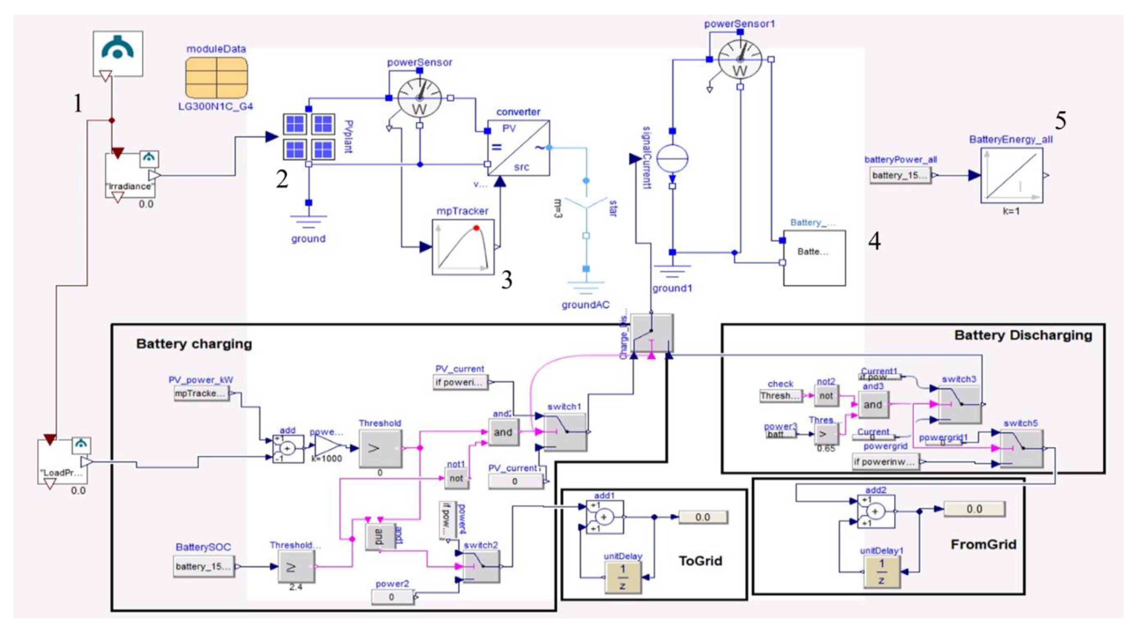
3.4. Electric Sub-System Model

The electric sub-systems include solar PV, batteries, power sensors, converter, and maximum power point tracker (MPPT) as the main components. The energy system is connected to the grid and net metering is active. The solar PV chosen for the simulations has a power output of 300 W and the model number is LG300N1C-G4. More details can be found in Appendix A.
Regarding the electrical storage, the model selected from the PhotoVoltaics library is a detailed one, including an open-circuit voltage (OCV) dependent on the state of charge (SoC), self-discharge, and internal resistances. The data for the circuitry modeling of the batteries were taken from the experimental results for lithium titanate oxide cells tested at CNR ITAE, as reported in Ref. [37]. The relevant data for a battery module is given below, in Table 3. The modules were then stacked in series to obtain the 5, 10, and 15 kWh capacities.
The control mechanism for battery management and energy exchange with the grid is shown in Figure 6. The control strategy initiates the process by first comparing the power from the PV panel with the required building load. In case the PV is generating power that is higher than required, the control strategy further checks the state of charge (SoC) of the batteries. If the SoC value is less than 0.8 (taken as the fully charged state of the battery), all the energy will be used to charge the batteries. Otherwise, the energy will be sent to the grid. Similarly, if the PV panels are producing less power than required, the SoC of the batteries will be checked; if it is greater than 0.2 (taken as the fully discharged state of a battery), then energy will be released from the batteries. Otherwise, energy will be acquired from the grid to meet the demand. It is worth noting that only a local exchange with energy generation and optimization was considered, instead of demand response services since, in the context of single-household residential users, they are still at the pilot stage in some of the analyzed countries.

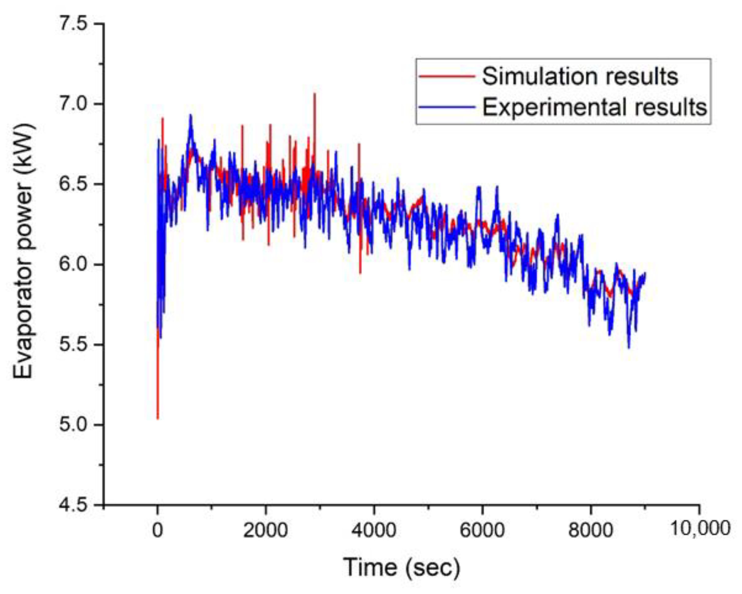
4. Reversible HP Model Validation

The model validation for the heat pump is carried out by comparing the experimental and simulation results. Specifically, the mass flow rates at the condenser and evaporator side and the HTF condenser and evaporator inlet temperatures from the experimental results were provided as input parameters to the model, while outlet temperatures in the HTF and refrigerant circuits and the pressure in the refrigerant circuits were used for calibration/validation purposes. A comparison of the simulation and experimental results for evaporator power at 2800 rpm is shown in Figure 7. It can be seen that the simulation results are in close proximity to the experimental results. The maximum deviation achieved for the results is within 10% of the experimental value; thus, they are in line with the measurement uncertainty. The results for other parameters and rpm can be seen in Figures S6–S13 in S2 (Supplementary Materials). This model can then be considered suitable for reproducing the behavior of the reversible heat pump.

5. Results and Discussion

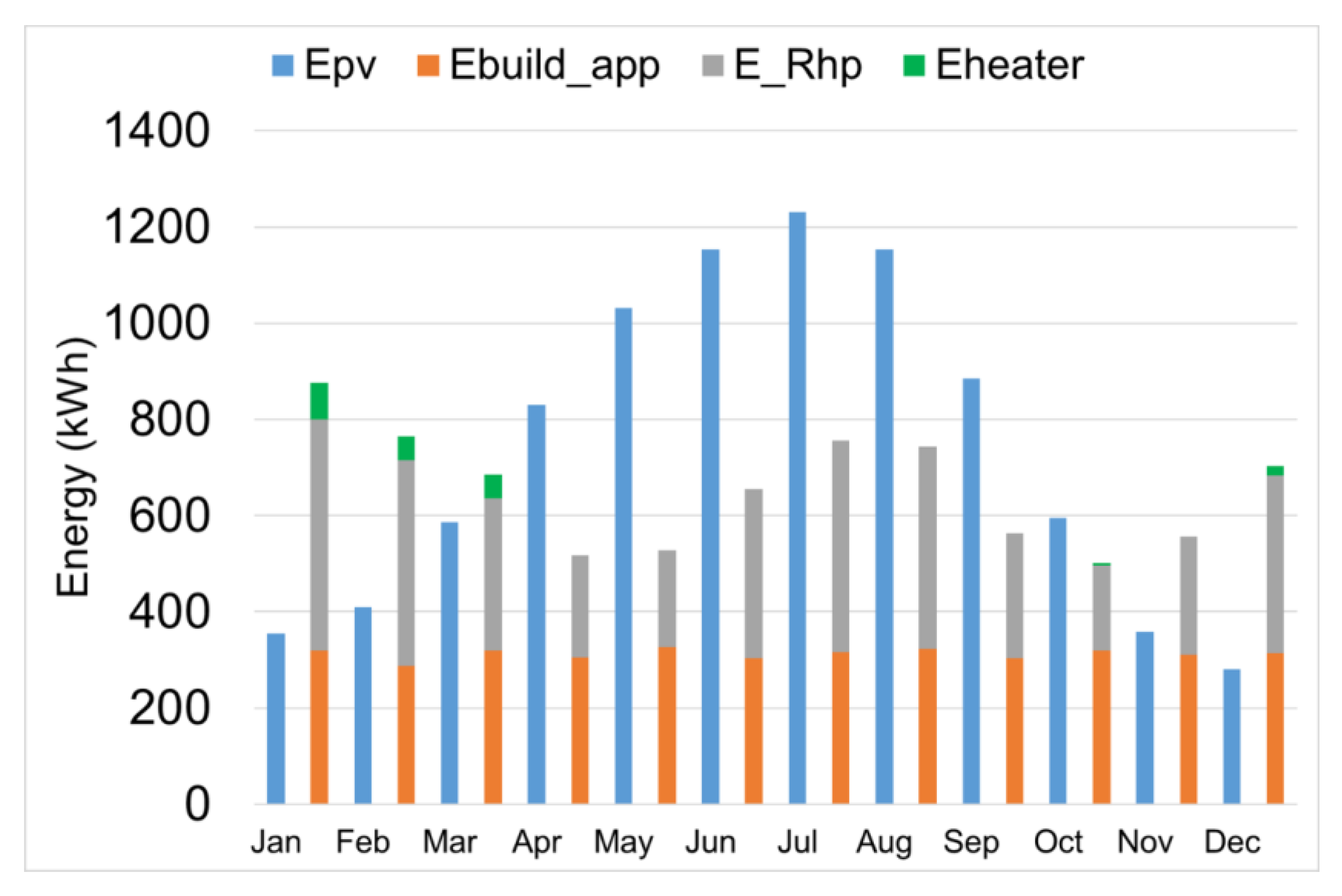
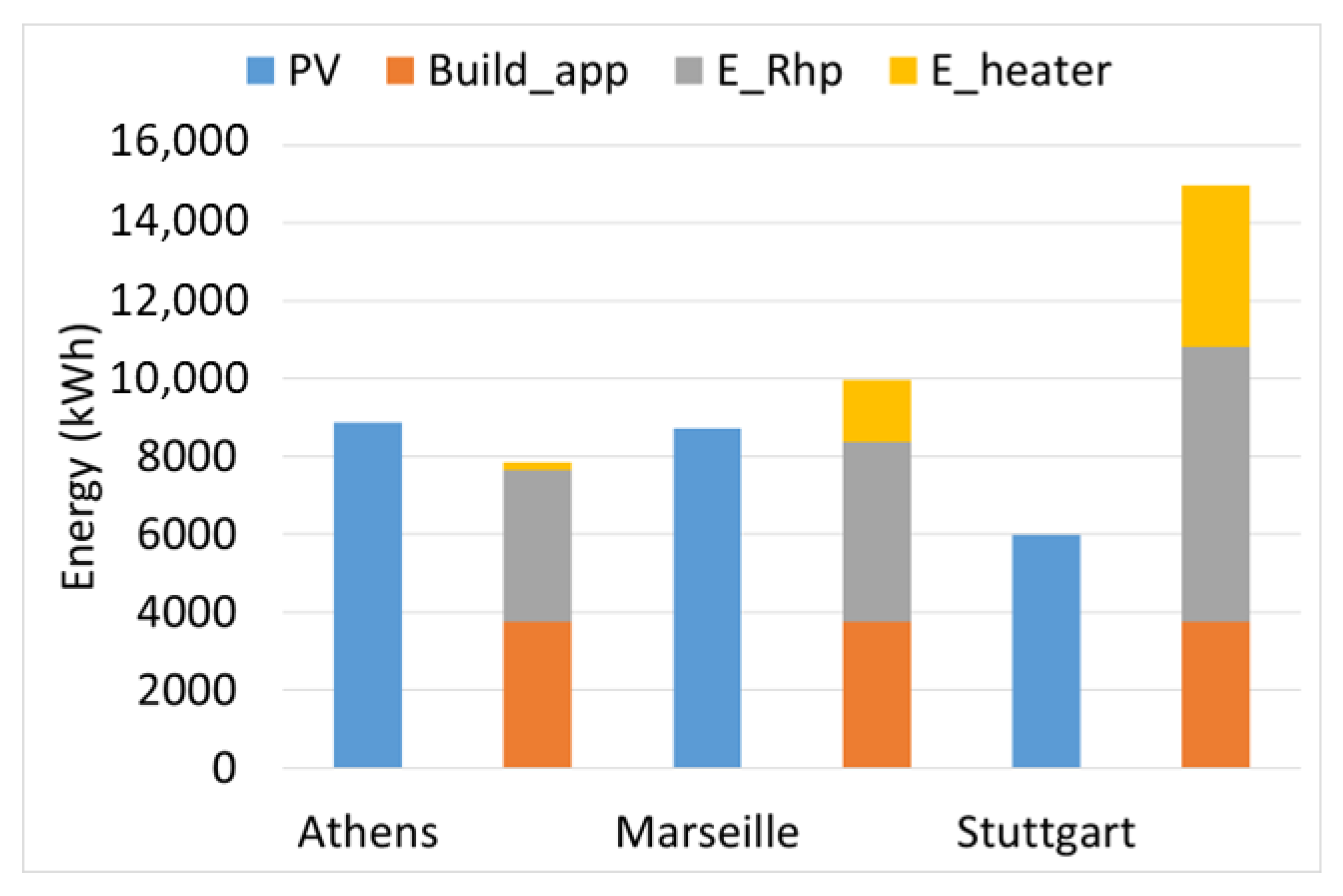
5.1. Results of Energy Analysis

5.1.1. Electricity Consumption

The system analyzed is only using electricity as the main energy carrier for covering the heating and cooling demand in Athens and Marseille; Stuttgart has a gas boiler as a backup source. The results in terms of energy consumption for the different components of the system throughout the year and for the three examined cities are presented in Figure 8, Figure 9 and Figure 10.
Figure 8 represents the energy that is produced and consumed in the case of Athens. In detail, it contains information about the energy produced by the PV (6 kWp) and energy consumed by the reversible HP compressor and building appliances. It also includes information about the electrical heater, which is used as a backup source. It can be seen that reversible HP consumption was high in January and July as these months demand the highest heating and cooling loads, respectively. Moreover, it can also be concluded that the reversible HP is adequate to meet both the heating and cooling demands and that a backup source is not required. As expected, during the winter, the electricity consumption is higher than the electricity production, whereas the opposite occurs during the summer. The average electricity consumption for the appliances is constant throughout the year and is about 300 kWh/month, whereas the consumption of the heat pump is extremely variable according to ambient conditions and varies from 200 kWh/month to 450 kWh/month.
Figure 9 represents a comparison of the energies produced by solar PV (6 kWp) and consumed by the building appliances and reversible HP for Marseille. It can be seen that the heat pump consumption is highest in the month of November, while the use of the backup source (an electric heater) is highest in January. For the summer season, the reversible HP has the highest operation in July. Moreover, it can be seen that the months of December and January are those in which greater use of the electrical heater is needed; this is due to the selected control logic, which shuts the HP down when the temperature drops below 0 °C. Increasing the HP size to also supply the energy needed for these two months would result in excessive costs and oversizing for the remaining months of the year. Possible future studies will consider the defrosting cycle of the HP as an alternative to the control logic selected. The consumption of the HP, if compared to the previous case, is lower during the summer (i.e., around 200 kWh/month, against 350 kWh/month) and much higher in the winter.
Figure 10 represents the histogram carrying information on the energy produced by solar PV (6 kWp) and the energy consumed by building appliances, the gas boiler, and the reversible HP in Stuttgart. Electricity and gas consumption are shown on different axes since gas is a primary energy source, while electricity is a secondary energy resource. Since the winter season is extreme in Stuttgart, the reversible HP has a higher share of the energy consumed in the winter months. Moreover, in sub-zero temperatures, the HP is turned off and energy is supplied through a gas boiler; therefore, the boiler’s consumption is high during the months of December, January, and February. In Athens, the energy produced by the PV exceeded that needed by the building for 8 months out of 12; in Marseille, this happened for 5 months out of 12, whereas in Stuttgart, the PV production only exceeded the building demand during the summer (May to August).
A yearly summary is presented in Figure 11 for all the examined cities. The energy values produced by solar PV (6 kWp) for Athens and Marseille are almost equal because of high solar irradiation, while this is low for Stuttgart. It can be seen that the use of reversible HP is high for Stuttgart, followed by Marseille and Athens, respectively. It is important to mention that the energy consumption shown for the heater in the case of Stuttgart is actually the consumption of a gas boiler. Energy consumption in terms of building area is 60.4 kWh/m2 for Athens, 76.6 kWh/m2 for Marseille, and 115 kWh/m2 for Stuttgart, respectively.

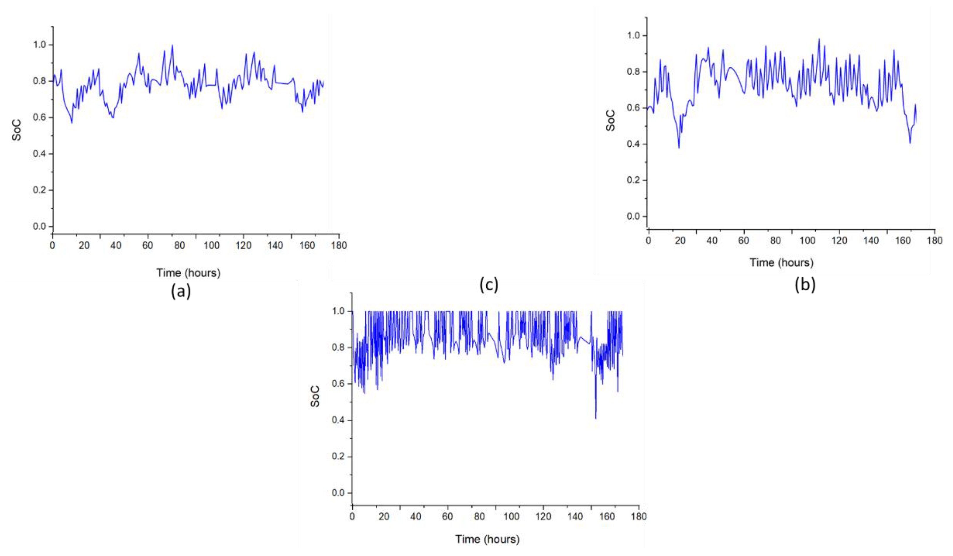
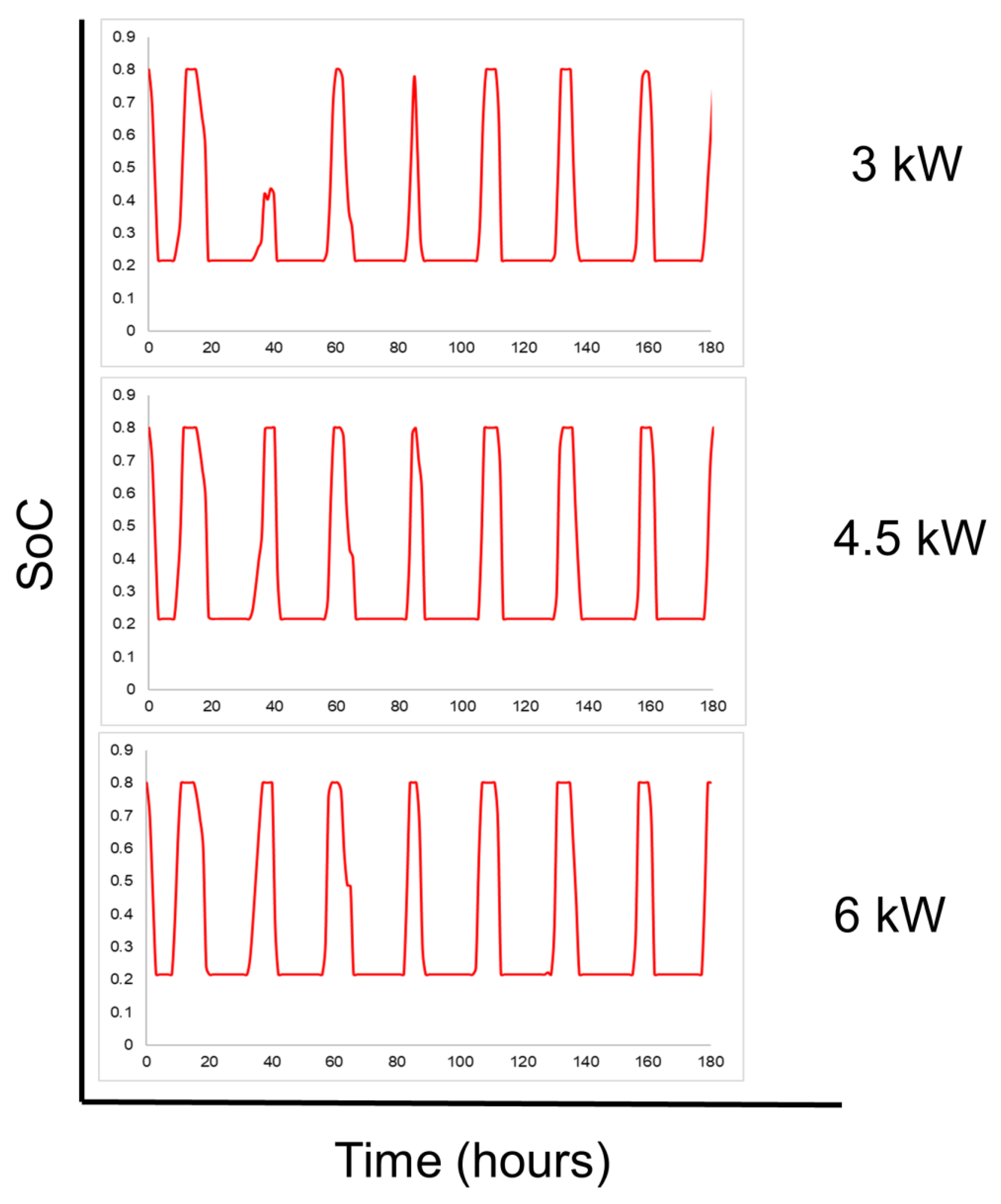
5.1.2. The Role of Energy Storage

One critical parameter when evaluating the overall energy yield of a renewable-based thermal system is the mismatch between energy production and energy request, which can only be mitigated by using energy storage systems [38]. In the present system, two storage types have been considered, thermal energy storage and electrical energy storage.
Figure 12 shows the state of charge (SoC) of the thermal energy storage tank for three cities for the second week of January, during the winter. The upper and lower limit of the SoC is actually the maximum and minimum temperatures in the tank during the winter season. The maximum temperature is given an SoC value of 1, while the lowest temperature receives an SoC value of 0. A linear equation is obtained using a two-point equation formula and SoC values for the rest of the temperatures in the storage tank are calculated. The SoC fluctuates between the maximum and minimum temperatures inside the storage tank. The temperature inside the storage tank varies because of the changing set-point temperature, which is a function of ambient temperature. The results for Stuttgart show that there is high heating demand throughout the week, which means that the HP and backup heater operate continuously. This, on the one hand, means that the SoC mostly remains between 0.8 and 1, which means that the set-point temperature is quite high because of the low ambient temperatures. On the other hand, a trend of rapid charge and discharge can be seen, which points toward high heating demand. Conversely, Athens is a cooling-dominated region; it can be seen that the ambient temperatures are not that low, as the SoC varies between 0.6 and 0.8. Moreover, the fluctuations are less frequent and smoother than in the case of Stuttgart. The results for Marseille show that heating demand is higher than in Athens and lower than in Stuttgart since the curve for the SoC presents more frequent fluctuations than in Athens but has a lower amplitude than in Marseille.
It is worth pointing out that the value of the SoC, especially for Athens and Marseille, which never drops below 0.5, indicates that the size of the storage is adequate for the system.
Figure 13 shows the SoC of the thermal energy storage tank for the summer in all three cities for the third week of July. It can be seen the curve of SoC for Athens is constricted, compared to Marseille and Stuttgart, which represents a constantly high cooling demand during the week. The rapid discharging and charging of the tanks also point to a high cooling demand. Conversely, the SoC for Stuttgart remains at 1 for most of the time in the week under consideration, which means that there is not a high cooling demand. The SoC curve for Marseille shows that the cooling demand is medium to high, as shown by the rapid charging and discharging of the tank. It is worth mentioning here that the set point for the summer season is 12 °C, while the reversible HP operates in a tolerance band of 2 °C. Therefore, the reversible HP is turned on when the temperature inside the tank reaches 14 °C (SoC value of 0) and is turned off when the temperature reaches 10 °C (SoC value of 1). Thus, the constant charging and discharging trend signals the high cooling demand.
Figure 14 contains the results for an SoC of 5 kWh battery size for Athens for the first week of January, using different PV sizes as the reference case. The maximum value for SoC is set as 0.8, while the lowest SoC value is 0.2. Therefore, at the maximum SOC, the battery will be considered fully charged, while at the SoC value of 0.2, the battery is considered to be in a dead state. The SoC of a battery can be defined as the ratio of available capacity to the maximum capacity of the battery. For the PV size of a 3-kW peak, it can be seen that the current produced results in a lower SoC in the batteries compared to other sizes. It is worth noting that the electric current that will charge the batteries results from the difference in the PV produced and the consumed power at building level. As the power produced by larger PV sizes will be high, this will result in higher currents being available to charge the batteries. The results for other battery and PV sizes are given in Figures S14–S16 in S2 (Supplementary Materials). In order to have more complete information on the behavior of electricity storage throughout the year, the effect on ambient conditions for the analyzed scenarios was evaluated.
Accordingly, Figure 15 contains the SoC as a function of ambient temperature for a 5-kWh battery size for the three cities. It can be seen that at lower temperatures, the SoC of the battery is close to the dead state because there is not enough solar irradiation during the winter season to charge the batteries. Conversely, the SoC for batteries is high in the summer season. Looking at the figures for Athens, the maximum SoC is reached when the ambient temperature is above 30 °C, as expected, since this corresponds to summer conditions. Interestingly, there is no significant difference between the 4.5 kW and 6 kW peaks. The differences between these PV sizes and the 3 kW cases are only evident during the summer and are in the order of 10%. In the case of Marseille, there is no significant difference between summer and winter conditions and the different PV sizes, which is mostly due to the limitations in solar intensity and the number of sun hours. In the case of Stuttgart, the average SoC is lower than for the other cities, due to geographical and climatic limitations. However, the benefit of the higher PV peak power during summer conditions is more evident than in the other cases. This is mostly due to the fact that the energy consumption from the heat pump in summer is lower; therefore, the energy accumulated for later use is higher. More details can be found in Figure S5 of S1 (Supplementary Materials).

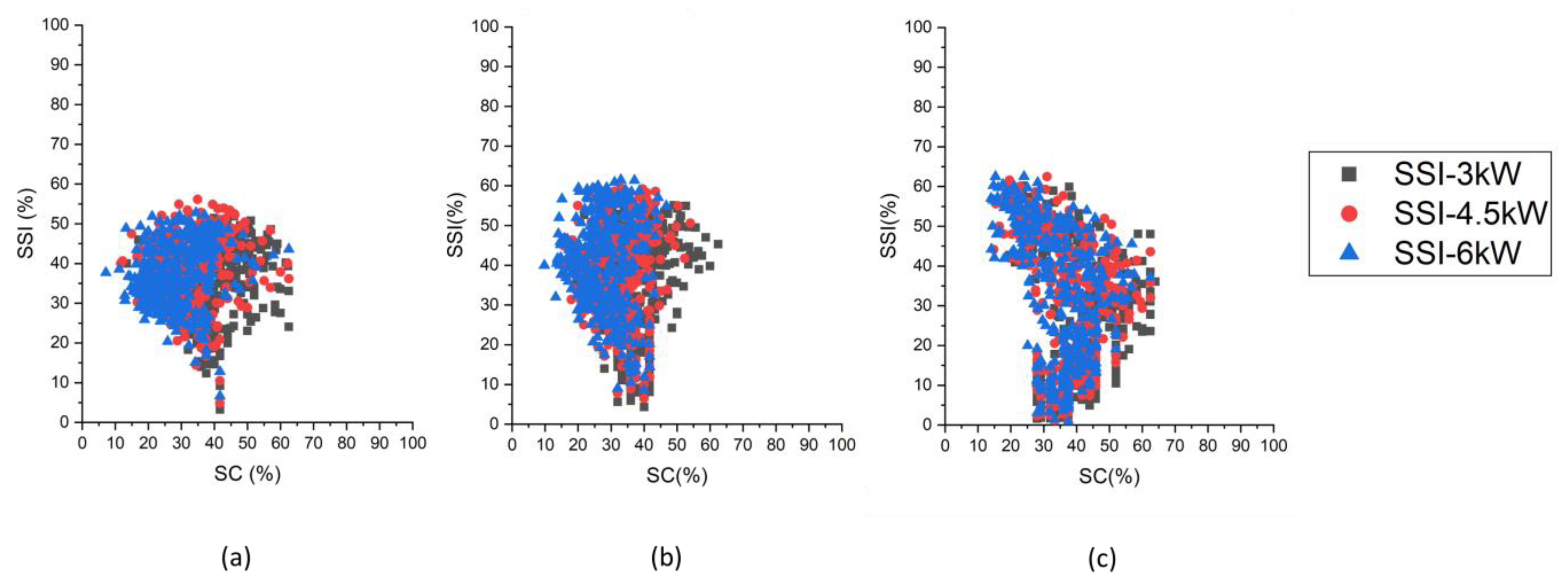
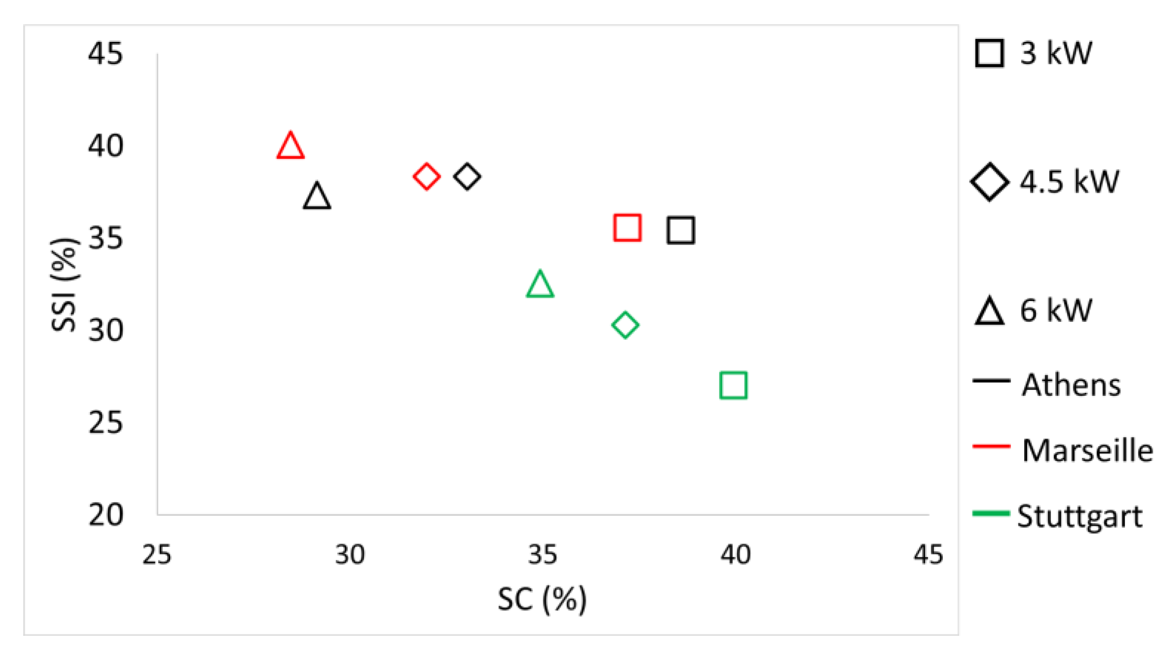
5.1.3. Self-Sufficiency and Energy Exchange with the Grid

One indicator that is often used to assess the techno-economic feasibility of an energy system is the self-sufficiency index (SSI). It is the ratio of locally produced energy via renewables for consumption to total energy consumption. A building with a high SSI index shows that the energy produced locally is being self-consumed and that there is little to no need for buying energy from the central grid. SSI is calculated using the following equation.
S S I = E P V E t o   g r i d E H P + E B u i l d i n g _ a p p l i a n c e s + E H e a t e r
Alongside SSI, another indicator used to assess techno-economic feasibility is self-consumption (SC). SC is the ratio of locally produced and consumed energy to total local generation. It is calculated using the following equation.
S C = E P V E t o   g r i d E P V
Both SSI and SC were calculated on an hourly basis. According to the calculations made for SSI, it was observed that increasing battery storage size has no effect on SSI value for the PV system sizes selected in the studies, which are those that are compatible with the surface area usually available in single-family houses. Therefore, it can be concluded that for all the households considered in the different cities in this study, a battery storage size of 5 kWh (the minimum size considered) is enough. In the upcoming graphs and calculations, a battery storage size of 5 kWh is assumed. Having a large-sized battery storage system is beneficial when the PV system is oversized, and excess energy can be stored for later use or sold to the grid. Moreover, having a large battery storage size is also beneficial when the sole purpose is to produce energy for selling to the grid. It is worth mentioning that according to the incentive policies of many European countries regarding PV installation, a customer receives more of an incentive when the aim is to increase self-consumption and not merely to sell energy back to the grid. Another important aspect to consider is the cost of batteries; it is not always cost-effective and economically feasible to have large battery sizes for households. These aspects will be further discussed in the following sections. For the upcoming economic calculations, a battery storage size of 5 kWh is used.
Figure 16 reports the monthly SSI values for Athens, Marseille, and Stuttgart for 6 kW solar PV panels. Increasing the PV power size and SSI index have a direct relationship as increasing the PV size results in higher values for the SSI index. Athens demonstrated the highest value of the SSI index since solar irradiance in the Mediterranean climate is high enough to cover a major portion of the energy demand of the energy system under observation. Using a PV size of 6 kW will help in achieving half of the energy demand in Marseille during the summer month of June. Stuttgart also reported a higher SSI index for the summer months, since electricity consumption is then lower. What is possible to see is that with the simulated system and a simple control strategy, in a strongly cooling-dominated climate such as Athens, the maximum SSI achieved was 0.9, while values ranging from 0.6 to 0.9 were reported for the entire year, indicating that, overall, less than 30% of the total energy demand from the building needed to be supplied by the external grid. In the case of Marseille, the average SSI was 0.5 for the entire year, indicating that half of the overall demand can still be met by internal production. In the case of Stuttgart, due to the high heating demand in winter and the lower solar irradiation, which reduced the available energy produced on the spot, it is still difficult to achieve independence from the main national energy grids with the selected layout. It is worth noting that in the case of Athens, there was overproduction from the PV in the summer, as highlighted in the previous sections, but the SSI was lower than 1. This is due to the fact that the times of energy production and requirement were also taken into account; therefore, on some occasions, the energy produced was higher than required and, thus, it was sold to the grid, which reduced the SSI value.
Figure 17 the SC vs SSI graph for Athens, Marseille, and Stuttgart. The data shown in this figure are for the whole year. It is possible to see that in the case of Athens, the different PV sizes were all grouped around the same SSI, whereas a spread in SC, which increased from 6 kW to 3 kW, was observed. In the cases of Marseille and Stuttgart, the SC was found within a narrower range, whereas a highly variable SSI was achieved.
To better analyze these results, Figure 18 shows the average values of SSI vs SC for three cities. It can be seen that self-consumption is higher for the 3-kW PV size since the maximum energy produced is utilized locally. As the PV size increases, the share of energy sold to the grid increases, which decreases the self-consumption value. SSI increases with increasing PV size as a larger share of the energy needs is fulfilled by locally produced energy with an increment in PV size. One exception is in the case of Athens, with a 6-kW PV size. In fact, for this PV size, the energy sold to the grid is higher than the energy purchased, as shown in Table 4, which reduces the available on-site energy to be consumed and reduces the SSI value. Stuttgart reported the highest SC values of around 40%, where the share of energy sent to the grid is quite low compared to that obtained from the grid. In addition, the energy requirement for Stuttgart is quite high because of extreme winter temperatures; thus, most of the energy produced on-site is consumed by building appliances. The lowest SC was reported by Marseille, which was around 28%, followed by Athens. The highest SSI was reported by Marseille, which was around 40%, followed by Athens (37%) and Stuttgart (32%).
Table 4 contains the details of the interaction of the energy system with the central grid. This entails the energy produced by each PV size and the energy bought and sold to the grid. The results show that increasing the PV size will result in selling more energy to the grid and buying less energy. In the case of Athens, the 6-kW PV size resulted in selling more energy to the grid than was purchased from it, which helps the system to achieve the payback time period relatively earlier. Among all three cities, Stuttgart has the lowest share of energy sold to the grid as most of the energy produced locally is consumed on-site. It is to be considered that an optimized PV size should be installed for a household since, at this level, the main aim of installing PV panels is to increase self-consumption rather than selling energy to the grid. Given the above considerations, it is important to mention that it is always important to quantify the cost savings that can be achieved when a new system is installed at a specific site. Moreover, this should also be considered if any economic incentives exist to encourage the establishment of new RES systems. Furthermore, an important aspect that needs to be taken into account is that the user must be able to quantify the cost savings and payback time since the investment costs may be high for HP [3,39]. Accordingly, in the next section, available subsidies in the analyzed countries are considered.

5.2. Economic Analysis

5.2.1. Main Assumptions

An economic analysis was carried out, taking into consideration the capital cost of the energy system and savings that can be possibly made by selling energy to the grid and using the saved energy in batteries. The cost of the energy system is given, component by component, in Table 5. The maintenance costs were considered to be EUR 400 per year for the energy system. Expenditures for pipes, pumps, the control system, and installation costs are taken to be 10% of the total capital cost. For all the components for which a reference from the literature is missing, the cost was considered by soliciting quotations from the different manufacturers.
The prices of electricity and gas used in calculations are given in Table 6. These prices include taxes and are for household consumers for the first half of the year 2022.
Capital expenditures (CAPEX) constitute the costs of all the components of the energy system. Equations for operating expenditures (OPEX), energy savings, and the discounted payback time period are given as follows in Equations (10)–(13).
O P E X = Energy _ fromGrid   ×   Electricity   price Energy _ toGrid   ×   Net _ metering   cos t + Energy _ from   Gas   ×   Gas   price +   Maintenance   cos t
A n n u a l   e n e r g y   s a v i n g s = ( Annual   energy   demand × E l e c t r i c i t y   p r i c e A c t u a l   a m o u n t   p a i d   a f t e r   n e t   m e t e r i n g ) +   O P E X   r e f e r e n c e   s y s t e m O P E X   u n d e r _ c o n s i d e r a t i o n   e n e r g y   s y s t e m
D i s c o u n t e d   p a y b a c k   t i m e   p e r i o d = A n n u a l   e n e r g y   s a v i n g s 1 + i n t e r e s t   r a t e n
In Equation (12), n stands for the compounding period in years. The interest rate for the discounted payback period is taken as 2.5% [49]. Consequently, the levelized cost of energy (LCOE) is calculated as per Equation (13). N stands for the lifetime period of the system, which is taken as 25 years.
L C O E = n = 0 N C A P E X 1 + i n t e r e s t   r a t e n + n = 1 N O P E X 1 + i n t e r e s t   r a t e n n 1 N T o t a l   e n e r g y   d e m a n d 1 + i n t e r e s t   r a t e n

5.2.2. Energy Policies and Subsidies for HP

A short description of the subsidies and energy policies of Greece, Germany, and France related to HP usage and the prices for net-metering for solar PV are given below. Over the last few decades, the prices of solar PV panels have dropped drastically, which makes it economically feasible to install them for households. This installation also comes with certain advantages, such as net-metering and feed-in tariff mechanisms, etc. Along with solar PV, wind turbines are also being installed locally to make a building self-sufficient in terms of meeting energy demand. There are three ways to use an RES integrated with the building [50]:
  • Working under a “feed-in-tariff” model, where all generated electricity, such as that from a PV system, is supplied to the grid.
  • Installing an autonomous off-grid system with storage batteries (e.g., utilizing PVs, wind turbines, etc.) that is independent of the grid, where all the energy from the RES is consumed.
  • Installing a renewable energy system that consumes as much energy as it produces, while remaining connected to the grid. When the energy demand is higher than the produced amount, energy is drawn from the grid. This is the concept of net metering.
The data from these policies are used for economic analysis.

Greece

The program “Energy saving at home II” aims at providing loans and tax-relief measures for energy-saving measures. The total budget of the program stands at EUR 292.43 million. The percentage funded by a subsidy or loan depends on the personal or family income of the applicant. There are seven brackets for income and the subsidy percentage can go as high as 70% [51].
Regarding the subsidies, there is an ongoing incentive program funded by the Greek state, called “EΞOIKONOMΩ 2021” (translated as “TO SAVE ENERGY 2021” in English), which, for an air/water heat pump of up to 8 kW nominal capacity, can fund up to EUR 4912.5 (75% × EUR 6550) and down to EUR 2620 (40% × EUR 6550), where EUR 6550 is the maximum threshold for an air/water heat pump of such a capacity (<8 kW—EUR 6550; <14 kW—EUR 8150; <20 kW—EUR 10,800). For geothermal heat pumps, the maximum threshold, based on the capacity, is: <8 kW—EUR 5650; <14 kW—EUR 7350; <20 kW—EUR 10,450 [52].
Regarding net metering, the policy says that the net consumption from the grid is calculated as the power absorbed minus the power produced. However, there is a clearance of net consumption every 3 years. This means that if the consumer has negative net consumption (i.e., power production) at the end of the three-year period, the “buffered” energy produced is lost and the consumer is not paid for it. This also means that at the beginning of the next 3-year period, the consumer does not have any stored energy in the grid. This measure was included in the legislation in order to avoid oversizing generation systems (e.g., PV), meaning that priority is given to the maximization of self-consumption of the produced power [53].

Germany

The Federal Office for Economic Affairs and Export Control (BAFA) offers financial support for heat energy produced in existing buildings using RES under the Market Incentive Program (MAP). Efficient aerothermal heat pumps with nominal heat outputs, up to and including 40 kW, will garner a minimum support payment of EUR 1500 for performance-controlled monovalent heat pumps and EUR 1300 for other aerothermal heat pumps (Guidelines for the Support of RES-H, Art. IV.3.2.1.1.). Air and air-heating pumps that transmit heat directly into the air are not supported (Guidelines for the Support of RES-H, Art. V.3.1.) [54]. More specific technical criteria and standards are outlined in Art. IV.3.1 and Art. IV.3.4 of the Guidelines for RES-H Support [54].
A bonus support payment of EUR 500 is given under the load-management scheme if the following two additional conditions are met: the concomitant construction of a buffer tank and compliance with the “Smart Grid-Ready” accreditation requirements. After complying with these conditions, a certificate is issued, which makes a consumer eligible to claim this discount.
The price of net metering for PV systems up to 10 kW is EUR 0.0860/kWh [55].

France

In an effort to reduce its reliance on gas, France has stopped providing subsidies for gas boilers and plan to increase the use of HP instead [56]. As a part of the government’s “resilience plan”, support will be provided for renewable energy heating and subsidies will be given to help households. The subsidy scheme, called “MaPrimeRenov”, is aimed at accelerating the installation of HP and biomass heaters. Another national program launched for the thermal renovation of buildings is called “habiter mieux”, which supports households with low incomes. Moreover, other funding schemes, such as the heat fund, “Fonds Chaleur”, and tax incentives also exist for installing HP and other renewable heating options such as biomass boilers [57].
According to the “MaPrimeRenov” scheme, there are four brackets that are defined based on each household’s income. More grants can be obtained via the use of CEE (certificats d’économies d’énergie) [58], which are not widely available except through Électricité de France (EDF). The grant for a Blue household, in the bracket with the least income, is set at EUR 4000.
The price of net metering in France for PV systems up to 10 kW is EUR 0.1/kWh [59].

5.2.3. Main Results

Table 7 contains the details related to capital costs, the subsidies provided under any governmental scheme, annual energy savings, and discounted payback periods for energy systems for the three cities studied. Economic analysis has been performed for three different PV sizes and for a single battery-storage size, i.e., 5 kWh. The payback time periods for Athens for all three PV sizes are quite close to each other. The results indicate that for the 6 kW PV size, despite a higher capital cost, the system will reach the break-even point in 3.9 years, which is comparable with the other two PV sizes, as energy sold to the grid is charged at a higher price than that purchased from the grid. Therefore, the consumer will end up saving money that needs to be paid to the electricity distribution companies in the absence of PV and a battery energy-storage system. Generally, at the household level, current European policies encourage households to have systems with high self-consumption and self-sufficiency, rather than systems designed with oversized PV and battery storage sizes in order to sell energy to the grid. The results for Marseille indicate that an energy system with a 3 kW PV size can reach the break-even point in 5.8 years, followed by 6.1 and 6.6 years, respectively, for the 4.5- and 6-kW PV sizes. The reported annual energy savings increase as the PV size increases, while the trend is the opposite in the case of Stuttgart. While simulating the system for a house in Stuttgart, the backup heater operates on gas. Since, during the winter, the HP cannot operate because of the extremely low and sub-zero temperatures, a major portion of the required energy is supplied by gas heaters. Therefore, the annual energy bills contain the contribution of both electricity and gas, while for the other two cities, only the electricity bill constitutes the annual energy bills. Moreover, the payback period is high for Stuttgart because of the high capital costs, low subsidies, and high energy prices. The discounted payback time period increases with the increase in PV size, as capital and maintenance costs become higher. Moreover, a rough estimate is made to check the importance of the subsidies offered by governments for energy system installation; it can be seen that the payback period increases by 1–2 years in all cases for all three cities. The configuration that shows the minimum payback time is for Athens, with a 3-kW PV size, while Stuttgart, with a 6-kW PV size configuration, has the maximum payback time period.
Table 8 contains details of all the associated costs for the reference system. The reference system for the winter period is a 24-kW gas boiler with 95% efficiency, while for the summer period, split air conditioners with a combined capacity of 10 kW, with a COP value of 2.5, are considered. Solar PV panels of three sizes, i.e., 3, 4.5, and 6 kW, are used to perform the economic analysis. Batteries are not considered for the reference system. For the reference system, a break-even time was calculated which is mainly due to the savings that can be achieved by selling the energy to the grid under the subsidy conditions described above. The discounted payback time period is higher, mainly because of the high operating costs. The results indicate that in the case of Athens, with a 3-kW system, the reference energy system will take almost twice the time to achieve the break-even point, compared to the energy system under observation. In the case of Marseille and a 3-kW system, the reference system will take almost 3 more years to achieve it than the studied system. Marseille reported relatively high payback periods compared to other cities because of the high annual energy bills as the climate is extreme in both summer and winter.

5.2.4. Levelized Cost of Electricity

The levelized cost of electricity (LCOE) is a metric used to evaluate and compare alternative energy production methods. It is considered as the average total cost of the energy-generating asset and its operating cost per unit of total electricity generated over its lifetime. The LCOE becomes important when a comparison is needed of the different energy-producing techniques, which have different span sizes, project sizes, and unequal capital costs and capacities. Figure 19 contains the results of the LCOE analysis for three cities with different PV sizes and 5-kWh battery size. Athens reported the lowest LCOE of EUR 0.18/kWh for a PV size of 6 kW, while Stuttgart reported the highest LCOE value of EUR 0.32/kWh for a 3-kW PV size. It can be seen that LCOE carries a decreasing trend as the PV size increases. With increasing PV size, the OPEX reduces as annual energy savings increase; thus, the LCOE is reduced as a result, despite an increase in capital cost. Athens reports lower LCOE values compared to other cities because of the lower capital and maintenance costs. As the associated costs increase in the case of Marseille and Stuttgart, the LCOE also increases.

6. Conclusions and Future Perspectives

This study focused on an analysis of the potentially widespread deployment of low-GWP heat pumps for heating and cooling provision, supported by onsite installed renewables and properly selected electric and thermal storage solutions.
An innovative heat pump was developed and tested, and the validated heat pump model was implemented along with other components in Modelica/Dymola to simulate the proposed energy system.
The analysis was performed for a single-family house in three reference cities, namely, Athens, Marseille, and Stuttgart, which were selected as representative cases for Mediterranean, hot semi-arid, and humid continental climates, respectively, according to the Köppen climate classification map. Simulations were performed to model the situation all year round and the results for the summer and winter seasons were presented and discussed, taking various on-site PV sizes and electric storage values.
The investigation tried to determine the interaction between the heat pump and thermal/electric storage, in order to maximize the self-sufficiency and the self-consumption of the system.
It turned out that for PV sizes typical of those in residential buildings, a battery size larger than 5 kWh does not provide any benefit in terms of the self-sufficiency index (SSI), while the SSI is strongly affected by the size of the PV system and the climatic conditions. In fact, a 6-kW PV system can reach quite high SSI values in summer in Athens (above 0.9), while it is limited to around 0.5 in Marseille and Stuttgart. Moreover, the proposed system was compared against a reference heating and cooling system, based on gas boilers and split air conditioners, showing a performance that was even more attractive than the reference system.
Furthermore, a techno-economic analysis was performed, analyzing the discounted payback time and the levelized cost of electricity (LCOE), also considering the energy policies and subsidies that are in place in several EU countries.
The achieved results demonstrated the possibility of achieving reasonable payback in Athens after around 3.8 years, which was much longer in Stuttgart, up to around 8 years. Similarly, the LCOE is much lower in Athens (i.e., down to EUR 0.18/kWh) compared to Stuttgart (i.e., EUR 0.32/kWh); this can be attributed to the capability of the system to be operated throughout the year, thanks to the greater level of electricity produced by the onsite PV, which is, of course, more limited in northern EU countries.
With the present study, the benefits of using an innovative HP with an unconventional low-GWP refrigerant under realistic operating conditions in a wide span of European climates were proven. In further studies, improvements to the HP layouts will be considered, including the possibility of DHW production, which is one of the main limitations in the current study, as well as the possibility of adding defrost cycles, which could extend further the operational conditions for the HP. This is especially necessary in view of the massive electrification foreseen in the next few years. Finally, the energy-selling mechanism could be modified, evaluating the possibility of further demand-response strategies.

Supplementary Materials

The following supporting information can be downloaded at: https://www.mdpi.com/article/10.3390/su15064973/s1, Figures S1–S5 are in Supplementary Materials S1 part; Figures S6–S16 are in Supplementary Materials S2 part.

Author Contributions

Conceptualization, O.A.R., V.P. and A.F.; methodology, O.A.R., V.P. and A.F.; software, O.A.R.; validation, O.A.R., V.P. and A.F.; formal analysis, O.A.R. and V.P.; investigation, O.A.R.; resources, A.F. and L.F.C.; data curation, A.F.; writing—original draft preparation, O.A.R.; writing—review and editing, V.P., A.F., L.F.C., A.C. and S.K.; visualization, O.A.R.; supervision, V.P., A.F. and L.F.C.; project administration, A.F., L.F.C., A.C. and S.K.; funding acquisition, A.F., A.C. and L.F.C. All authors have read and agreed to the published version of the manuscript.

Funding

This project has received funding from the European Union’s Horizon 2020 research and innovation program under grant agreement No 814945 (SolBio-Rev). This work was partially funded by the Ministerio de Ciencia e Innovación de España (PID2021-123511OB-C31-MCIN/AEI/10.13039/501100011033/FEDER, UE).

Institutional Review Board Statement

Not applicable.

Informed Consent Statement

Not applicable.

Data Availability Statement

Data will be made available on request to the corresponding author.

Acknowledgments

The authors at UdL would like to thank the Catalan Government for the quality accreditation given to their research group, GREiA (2017 SGR 1537). GREiA is a certified agent TECNIO in the category of technology developers, from the Government of Catalonia. This work is partially supported by ICREA under the ICREA Academia program.

Conflicts of Interest

The authors declare no conflict of interest.

Acronyms

European UnionEU
heating, ventilation, and air-conditioningHVAC
global warming potentialGWP
nearly zero-energy buildingsnZEB
renewable energy sources RES
seasonal coefficient of performance SCOP
self-sufficiency indexSSI
heat pumpHP
levelized cost of energyLCOE
high temperatureHT
low temperatureLT
medium temperatureMT
heat transfer fluidHTF
logarithmic mean temperature differenceLMTD
energy efficiency ratioEER
functional mock-up interfaceFMI
maximum power point tracker MPPT
open circuit voltageOCV
state of chargeSoC

Appendix A

Appendix A.1. Thermal Sub-System Model Components

A brief detail of all the thermal components used for modeling is given below. The overall Dymola layout for the thermal sub-system is shown in Figure A1.
Figure A1. HP model: 1—Data input files; 2—Condenser; 3—Heater control; 4—Evaporator; 5—Storage tank; 6—Compressor control; 7—Compressor; 8—Expansion valve; 9—Calculation blocks; 10—Separator; 11—Filling station; 12—Applying heating/cooling load.
Sustainability 15 04973 g0a1

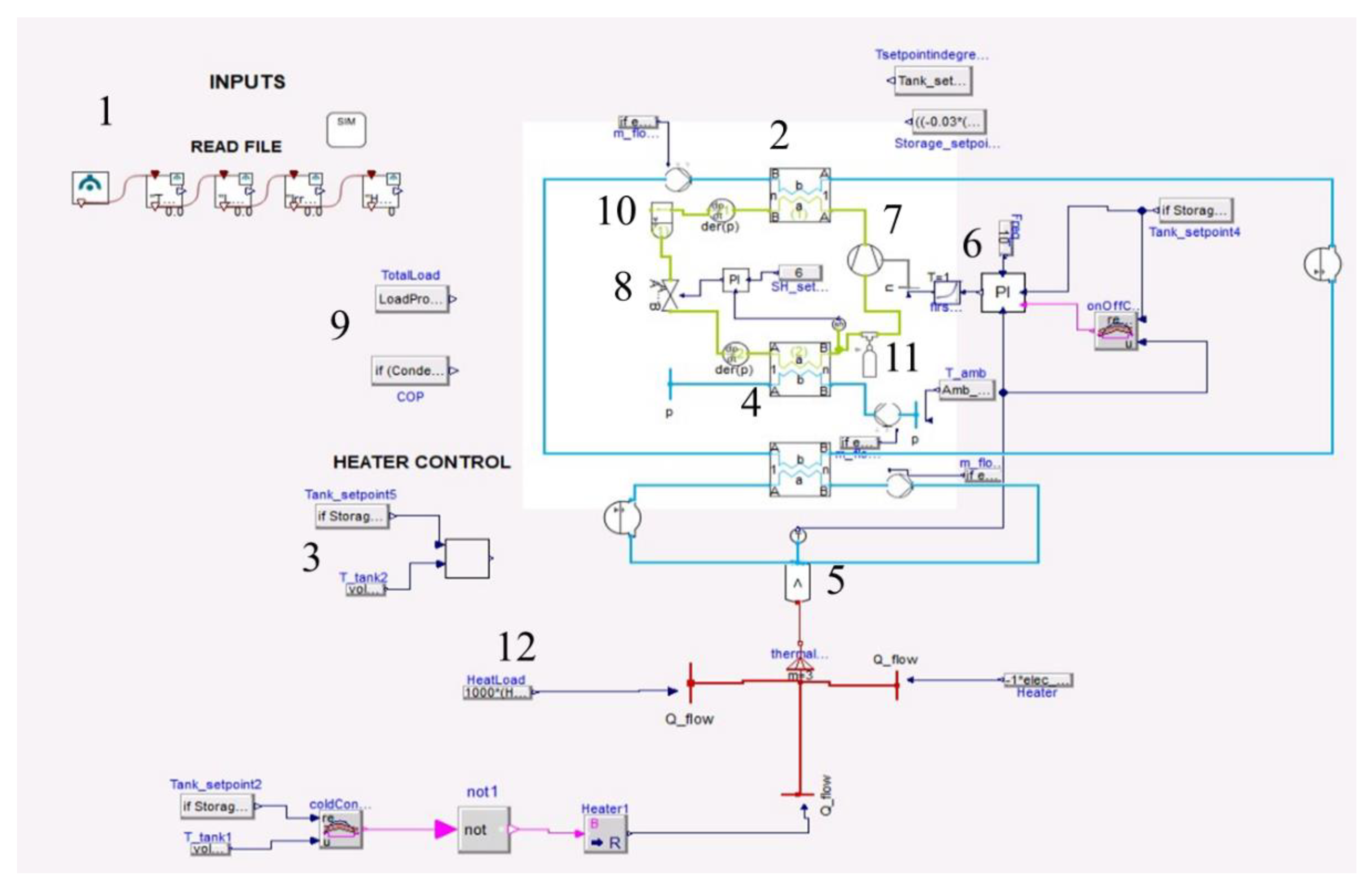
Appendix A.1.1. Condenser and Evaporator

The parallel flow plate heat exchanger models from TIL libraries are used for the condenser and evaporator. The wall material is stainless steel, and a geometry-based conduction model is used for the heat conduction model. A zero-pressure-drop model is used for both the refrigerant and liquid. General details of heat exchangers are given in Table A1, below. A condenser has 36 plates, while an evaporator has 40 plates.
Table A1. Heat exchanger details for the model of the evaporator and condenser.
Heat Exchangers (HX)
TypePlate Heat Exchanger
UA Condenser (W/K)7132
UA Evaporator (W/K)11,379
Condenser heat transfer area (m2)1.06
Evaporator heat transfer area (m2)1.18
RefrigerantR1234ze(E)
Heat transfer fluidWater

Appendix A.1.2. Compressor

An efficiency-based compressor is used for HP modeling, which operates based on three efficiencies, namely, volumetric, isentropic, and effective isentropic efficiency. Volumetric efficiency is the ratio of the actual mass flow rate to the theoretically possible mass flow rate. Isentropic efficiency can be defined as the ratio of enthalpy increase during an isentropic compression to the actual enthalpy increase during the compression. Similarly, the ratio of isentropic enthalpy, transported to the refrigerant, to the supplied mechanical power represents effective isentropic efficiency. The values for the volumetric efficiency, isentropic efficiency, and effective isentropic efficiency were determined as the fitting parameters from the experimental results and were considered equal to 1, 0.55, and 0.88, respectively.

Appendix A.1.3. Expansion Valve

An orifice valve is used with an effective area input that is controlled by a PI controller, which regulates the opening of the valve based on input signals from the superheating sensor and superheating set point. The set point for superheating is set as 6 K. The size of the expansion valve selected is compatible with the one that was actually installed on the prototype.

Appendix A.1.4. Liquid Separator

A separator is used to segregate the refrigerant into its vapor and liquid forms. The model requires the volume and filling levels as inputs. The ideal separation characteristic is selected by default; it behaves as follows. If the filling level is between 10% and 90%, the gas and liquid ports provide pure gaseous and liquid conditions, respectively. If the filling level is lower than 10%, the liquid port provides a mixture of gaseous and liquid conditions. If the filling level is higher than 90%, the gas port provides a mixture of gaseous and liquid conditions, depending on the filling level.

Appendix A.1.5. Thermal Energy Storage Tank

A liquid volume model is used as a thermal energy storage tank, which is a stirred vessel with one mixed temperature inside it. The tank also has a heat port, which can be used as the electrical heater input or when applying it for cooling and heating loads.

Appendix A.2. Thermal Sub-System Control and Management

Appendix A.2.1. Heater Control

The auxiliary heater comes into play when the HP is already working at its full capacity but is unable to meet the demand. The HP operation is confined within the tolerance band of 2 °C above and below the set point. If the temperature drops 4 degrees below the set point, the electric heater comes into action and turns off once the temperature reaches 2 degrees above the set point. In the case of Athens, an auxiliary heater of 3 kW was used, whereas for Marseille, a heater of 5 kW was used, while for Stuttgart, a gas boiler of 15 kW was used since the required heating load is quite high during the winter.

Appendix A.2.2. Expansion Valve Control

Valve opening is controlled by a PI controller, which takes its input from a superheating (SH) sensor. The value for SH is set at 6 K. Based on this set value, the controller adjusts the valve opening to make sure that the SH taking place is at 6 K.

Appendix A.2.3. HTF Mass Flow Control

Pumps have been used to regulate the HTF flow in the circuits on the condenser and evaporator sides. These pumps are controlled through the mass flow rate input, which varies linearly with the part load of the heat pump, with a maximum of 0.62 kg/s for a full load. If the storage temperature drops below the given threshold (in summer), the compressor will be turned on (or the frequency will be increased if it has already been working) and the expansion valve will function in order to keep the refrigerant temperature at 6 K at the evaporator outlet. The pumps will also then be turned on at full capacity.

Appendix A.3. Electric Sub-System Model Components

PV and Auxiliaries

The Dymola diagram for the electric subsystem is shown in Figure A2. Standard models from the PhotoVoltaics library were used. The data for the PV systems are taken from LG monocrystalline 300 W cells [60], arranged in strings of 5 modules. The azimuth is zero, while the tilt angle is at 45 degrees. The number of strings depends on the peak power selected for the PV plant. An ideal converter was considered for the DC to AC signal conversion. The main features of the PV cells are given in Table A2.
Table A2. Electrical properties of the PV panel (standard test conditions; irradiance 1000 W/m2, module temperature 25 °C, air mass (AM) 1.5).
Electrical Properties (STC)
Power Output (W)300
Cells6 × 10
Cell vendorLG
Cell typeMonocrystalline/N-type
MPP voltage (Vmpp) (V)32.2
MPP current (Impp) (A)9.34
Open circuit voltage (V)39.8
Short circuit current (A)9.9
Module efficiency (%)18.3
Figure A2. Battery storage and management system: 1—Input data; 2—PV panel; 3—MPPT tracker; 4—Battery storage; 5—Blocks for energy calculations.
Sustainability 15 04973 g0a2

References

  1. Archive: Consumption of Energy-Statistics Explained. Available online: https://ec.europa.eu/eurostat/statistics-explained/index.php?title=Archive:Consumption_of_energy (accessed on 16 November 2022).
  2. Economidou, M.; Atanasiu, B.; Despret, C.; Maio, J.; Nolte, I.; Rapf, O.; Laustsen, J.; Ruyssevelt, P.; Staniaszek, D.; Strong, D.; et al. Europe’s Buildings under the Microscope. A Country-by-Country Review of the Energy Performance of Buildings. Buildings Performance Institute Europe (BPIE). 2011. Available online: https://bpie.eu/wp-content/uploads/2015/10/HR_EU_B_under_microscope_study.pdf (accessed on 16 November 2022).
  3. Di Perna, C.; Magri, G.; Giuliani, G.; Serenelli, G. Experimental Assessment and Dynamic Analysis of a Hybrid Generator Composed of an Air Source Heat Pump Coupled with a Condensing Gas Boiler in a Residential Building. Appl. Therm. Eng. 2015, 76, 86–97. [Google Scholar] [CrossRef]
  4. Rehman, O.A.; Palomba, V.; Frazzica, A.; Cabeza, L.F. Enabling Technologies for Sector Coupling: A Review on the Role of Heat Pumps and Thermal Energy Storage. Energies 2021, 14, 8195. [Google Scholar] [CrossRef]
  5. Kolokotsa, D.; Rovas, D.; Kosmatopoulos, E.; Kalaitzakis, K. A Roadmap towards Intelligent Net Zero- and Positive-Energy Buildings. Sol. Energy 2011, 85, 3067–3084. [Google Scholar] [CrossRef]
  6. Kapsalaki, M.; Leal, V.; Santamouris, M. A Methodology for Economic Efficient Design of Net Zero Energy Buildings. Energy Build. 2012, 55, 765–778. [Google Scholar] [CrossRef]
  7. Apache, P. EN Horizon 2020 Work Programme 2018–2020 10. Secure, Clean and Efficient Energy. 2020. Available online: https://policycommons.net/artifacts/2024173/en-horizon-2020-work-programme-2018-2020-10/2776616/ (accessed on 16 November 2022).
  8. D’Agostino, D.; Zangheri, P.; Castellazzi, L. Towards Nearly Zero Energy Buildings in Europe: A Focus on Retrofit in Non-Residential Buildings. Energies 2017, 10, 117. [Google Scholar] [CrossRef]
  9. Zanetti, E.; Aprile, M.; Kum, D.; Scoccia, R.; Motta, M. Energy Saving Potentials of a Photovoltaic Assisted Heat Pump for Hybrid Building Heating System via Optimal Control. J. Build. Eng. 2020, 27, 100854. [Google Scholar] [CrossRef]
  10. Li, G. Parallel Loop Configuration for Hybrid Heat Pump–Gas Fired Water Heater System with Smart Control Strategy. Appl. Therm. Eng. 2018, 138, 807–818. [Google Scholar] [CrossRef]
  11. Thieblemont, H.; Haghighat, F.; Ooka, R.; Moreau, A. Predictive Control Strategies Based on Weather Forecast in Buildings with Energy Storage System: A Review of the State-of-the Art. Energy Build. 2017, 153, 485–500. [Google Scholar] [CrossRef] [Green Version]
  12. Bagarella, G.; Lazzarin, R.; Noro, M. Annual Simulation, Energy and Economic Analysis of Hybrid Heat Pump Systems for Residential Buildings. Appl. Therm. Eng. 2016, 99, 485–494. [Google Scholar] [CrossRef]
  13. Chen, Y.; Chen, Z.; Chen, Z.; Yuan, X. Dynamic Modeling of Solar-Assisted Ground Source Heat Pump Using Modelica. Appl. Therm. Eng. 2021, 196, 117324. [Google Scholar] [CrossRef]
  14. Beccali, M.; Finocchiaro, P.; Ippolito, M.G.; Leone, G.; Panno, D.; Zizzo, G. Analysis of Some Renewable Energy Uses and Demand Side Measures for Hotels on Small Mediterranean Islands: A Case Study. Energy 2018, 157, 106–114. [Google Scholar] [CrossRef]
  15. Eslami, S.; Gholami, A.; Bakhtiari, A.; Zandi, M.; Noorollahi, Y. Experimental Investigation of a Multi-Generation Energy System for a Nearly Zero-Energy Park: A Solution toward Sustainable Future. Energy Convers. Manag. 2019, 200, 112107. [Google Scholar] [CrossRef]
  16. Ciriminna, R.; Pagliaro, M.; Meneguzzo, F.; Pecoraino, M. Solar Energy for Sicily’s Remote Islands: On the Route from Fossil to Renewable Energy. Int. J. Sustain. Built Environ. 2016, 5, 132–140. [Google Scholar] [CrossRef] [Green Version]
  17. Calise, F.; Dentice d’Accadia, M.; Figaj, R.D.; Vanoli, L. Thermoeconomic Optimization of a Solar-Assisted Heat Pump Based on Transient Simulations and Computer Design of Experiments. Energy Convers. Manag. 2016, 125, 166–184. [Google Scholar] [CrossRef]
  18. Calise, F.; Cappiello, F.L.; Dentice d’Accadia, M.; Vicidomini, M. Dynamic Modelling and Thermoeconomic Analysis of Micro Wind Turbines and Building Integrated Photovoltaic Panels. Renew. Energy 2020, 160, 633–652. [Google Scholar] [CrossRef]
  19. Roselli, C.; Tariello, F.; Sasso, M. Integration of a Photovoltaic System with an Electric Heat Pump and Electrical Energy Storage Serving an Office Building. J. Sustain. Dev. Energy Water Environ. Syst. 2019, 7, 213–228. [Google Scholar] [CrossRef] [Green Version]
  20. Ma, R.; Qiao, H.; Yu, X.; Yang, B.; Yang, H. Thermo-Economic Analysis and Multi-Objective Optimization of a Reversible Heat Pump-Organic Rankine Cycle Power System for Energy Storage. Appl. Therm. Eng. 2023, 220, 119658. [Google Scholar] [CrossRef]
  21. Cirone, D.; Bruno, R.; Bevilacqua, P.; Perrella, S.; Arcuri, N. Techno-Economic Analysis of an Energy Community Based on PV and Electric Storage Systems in a Small Mountain Locality of South Italy: A Case Study. Sustainability 2022, 14, 13877. [Google Scholar] [CrossRef]
  22. Global Warming Potential Values of Hydrofluorocarbon Refrigerants-DCCEEW. Available online: https://www.dcceew.gov.au/environment/protection/ozone/rac/global-warming-potential-values-hfc-refrigerants (accessed on 17 December 2022).
  23. Alabdulkarem, A.; Eldeeb, R.; Hwang, Y.; Aute, V.; Radermacher, R. Testing, Simulation and Soft-Optimization of R410A Low-GWP Alternatives in Heat Pump System. Int. J. Refrig. 2015, 60, 106–117. [Google Scholar] [CrossRef]
  24. Palomba, V.; Dino, G.E.; Frazzica, A. Coupling Sorption and Compression Chillers in Hybrid Cascade Layout for Efficient Exploitation of Renewables: Sizing, Design and Optimization. Renew. Energy 2020, 154, 11–28. [Google Scholar] [CrossRef]
  25. Dino, G.E.; Palomba, V.; Nowak, E.; Frazzica, A. Experimental Characterization of an Innovative Hybrid Thermal-Electric Chiller for Industrial Cooling and Refrigeration Application. Appl. Energy 2021, 281, 116098. [Google Scholar] [CrossRef]
  26. Application Note Thermal Energy Storage Strategies for Commercial HVAC Systems. 1997. Available online: https://www.pge.com/includes/docs/pdfs/about/edusafety/training/pec/inforesource/thrmstor.pdf (accessed on 17 December 2022).
  27. Residential Geothermal Water Source Chiller and Heat Pump of 10 kw-Buy Residential Heat Pump, Domestic Heat Pump, Ground Source Heat Pump Product on Alibaba.Com. Available online: https://www.alibaba.com/product-detail/Residential-Geothermal-Water-Source-Chiller-And_1600744659947.html?s=p (accessed on 17 December 2022).
  28. Daikin Applied EWAQ010ACV3P Air Cooled Mini Inverter Water Chiller 10 Kw/34000Btu 240 V 50 Hz. Available online: https://www.orionairsales.co.uk/daikin-applied-ewaq010acv3p-air-cooled-mini-inverter-water-chiller-10kw34000btu-240v50hz-10472-p.asp (accessed on 17 December 2022).
  29. Daikin Scroll Chiller EWWQ-KC-Daikin Applied Europe. Available online: https://www.daikinapplied.eu/products/daikin-scroll-chiller-ewwq-kc/ (accessed on 17 December 2022).
  30. Dymola-Dassault Systèmes®. Available online: https://www.3ds.com/products-services/catia/products/dymola/ (accessed on 25 November 2022).
  31. TIL Suite. Available online: https://www.tlk-thermo.com/index.php/en/software/38-til-suite (accessed on 17 December 2022).
  32. Brkic, J.; Ceran, M.; Elmoghazy, M.; Kavlak, R.; Kral, C. PhotoVoltaics Library. Available online: https://build.openmodelica.org/Documentation/PhotoVoltaics.html (accessed on 17 December 2022).
  33. Vasta, S.; Palomba, V.; Frazzica, A.; Di Bella, G.; Freni, A. Techno-Economic Analysis of Solar Cooling Systems for Residential Buildings in Italy. J. Sol. Energy Eng. Trans. ASME 2016, 138, 031005. [Google Scholar] [CrossRef]
  34. Longo, S.; Palomba, V.; Beccali, M.; Cellura, M.; Vasta, S. Energy Balance and Life Cycle Assessment of Small Size Residential Solar Heating and Cooling Systems Equipped with Adsorption Chillers. Sol. Energy 2017, 158, 543–558. [Google Scholar] [CrossRef]
  35. Richardson, I.; Thomson, M. Accredited PV Measurement and Calibration Lab|CREST|Loughborough University. Available online: https://www.lboro.ac.uk/research/crest/working-with-us/lab/ (accessed on 21 April 2021).
  36. Interactive Europe Koppen-Geiger Climate Classification Map. Available online: https://www.plantmaps.com/koppen-climate-classification-map-europe.php (accessed on 11 December 2022).
  37. Palomba, V.; Bonanno, A.; Brunaccini, G.; Aloisio, D.; Sergi, F.; Dino, G.E.; Varvaggiannis, E.; Karellas, S.; Nitsch, B.; Strehlow, A.; et al. Hybrid Cascade Heat Pump and Thermal-Electric Energy Storage System for Residential Buildings: Experimental Testing and Performance Analysis. Energies 2021, 14, 2580. [Google Scholar] [CrossRef]
  38. Cabeza, L.F.; Palomba, V. The Role of Thermal Energy Storage in the Energy System. In Reference Module in Earth Systems and Environmental Sciences; Elsevier: Amsterdam, The Netherlands, 2020. [Google Scholar]
  39. Keinath, C.M.; Garimella, S. An Energy and Cost Comparison of Residential Water Heating Technologies. Energy 2017, 128, 626–633. [Google Scholar] [CrossRef]
  40. Ferreira, A.C.; Silva, A.; Teixeira, J.C.; Teixeira, S. Multi-Objective Optimization of Solar Thermal Systems Applied to Portuguese Dwellings. Energies 2020, 13, 6739. [Google Scholar] [CrossRef]
  41. 220 v 500 w 800 w 1500 w 2 kw 3 kw 4000 w 4 kw 6 kw 9 kw 12 kw 15 kw 20 kw 30 kw Electric Resistance Flange Immersion Water Heater Element-Buy 110 v Immersion Heater, 240 v Immersion Heater, 6 kw Stainless Steel Immersion Heater Product on Alibaba.Com. Available online: https://www.alibaba.com/product-detail/Water-Immersion-Flange-Heater-220v-500w_1881524500.html?s=p (accessed on 10 December 2022).
  42. LG300N1C-G4 NeON2. Available online: https://www.europe-solarstore.com/lg300n1c-g4-neon2-174.html (accessed on 10 December 2022).
  43. Innovative Compact HYbrid Electrical/Thermal Energy Storage Systems for Low Energy BUILDings Life Cycle Cost Assessment Studies. Available online: http://www.hybuild.eu/wp-content/uploads/2022/12/HYBUILD-D5.3.pdf (accessed on 10 December 2022).
  44. Baxi 615 Gas System Condensing Boiler|Boilers|Screwfix.Com. Available online: https://www.screwfix.com/p/baxi-615-gas-system-condensing-boiler/563hg (accessed on 15 December 2022).
  45. Worcester Greenstar Ri 24 kW Heat Only Gas Boiler ERP 7733600311|Travis Perkins. Available online: https://www.travisperkins.co.uk/regular-gas-boilers/worcester-greenstar-ri-24kw-heat-only-gas-boiler-erp-7733600311/p/263628 (accessed on 10 December 2022).
  46. 5 kW LG Standard Wall Mounted Unit. Available online: https://cooleasy.co.uk/lg-standard-3-5kw-air-con-heat-pump-system.html (accessed on 16 December 2022).
  47. Natural Gas Price Statistics-Statistics Explained. Available online: https://ec.europa.eu/eurostat/statistics-explained/index.php?title=Natural_gas_price_statistics (accessed on 12 December 2022).
  48. Electricity Price Statistics-Statistics Explained. Available online: https://ec.europa.eu/eurostat/statistics-explained/index.php?title=Electricity_price_statistics (accessed on 12 December 2022).
  49. Key ECB Interest Rates. Available online: https://www.ecb.europa.eu/stats/policy_and_exchange_rates/key_ecb_interest_rates/html/index.en.html (accessed on 17 December 2022).
  50. Net Metering. Available online: https://www.c2h.gr/en/renewable-energy/net-metering (accessed on 11 December 2022).
  51. Renewable Energy Policy Database and Support: Single. Available online: http://www.res-legal.eu/en/search-by-country/greece/single/s/res-hc/t/promotion/aid/subsidy-ii-combined-with-loan-energy-saving-at-home-ii/lastp/139/ (accessed on 12 December 2022).
  52. Ministry of Environment and Energy, Greece. Oδηγός Eφαρμογής Προγράμματος «EΞOIKONOMΩ 2021» [Application Guide of “TO SAVE ENERGY 2021” Program]. 2021. Available online: https://exoikonomo2021.gov.gr/odegos (accessed on 16 December 2022).
  53. Government Gazette Greece 3971/Β/30-08-2021, Amendment of the Ministry of Environment and Energy/15084/382/19.02.2019 Ministerial Decision Installation of Power Plants by Self-Producers with the Application of Net-Metering or Virtual Net-Metering Accordi. 2021. Available online: https://exoikonomo2021.gov.gr/opheloumenoi (accessed on 17 December 2022).
  54. Renewable Energy Policy Database and Support: Single. Available online: http://www.res-legal.eu/en/search-by-country/germany/single/s/res-hc/t/promotion/aid/subsidy-investment-support/lastp/135/ (accessed on 10 December 2022).
  55. Marian Willhun Germany Raises Feed-In Tariffs for Solar up to 750 KW–Pv Magazine International. Available online: https://www.pv-magazine.com/2022/07/07/germany-raises-feed-in-tariffs-for-solar-up-to-750-kw/ (accessed on 10 December 2022).
  56. Geert de Clerq France Ends Gas Heaters Subsidies, Boosts Heat Pumps in Bid to Cut Russia Reliance|Reuters. Available online: https://www.reuters.com/world/europe/france-ends-gas-heaters-subsidies-boosts-heat-pumps-bid-cut-russia-reliance-2022-03-16/ (accessed on 10 December 2022).
  57. Renewable Energy Policy Database and Support: Tools List. Available online: http://www.res-legal.eu/en/search-by-country/france/tools-list/c/france/s/res-hc/t/promotion/sum/132/lpid/131/ (accessed on 12 December 2022).
  58. Home Energy Conservation Tax Credits in France (Crédit d’impot Développement Durable). Available online: https://www.french-property.com/guides/france/building/renovation/energy-conservation (accessed on 10 December 2022).
  59. Does the Installation of Solar Panels in France Make Sense?|French-Property.Com. Available online: https://www.french-property.com/news/money_france/installation_solar_panels (accessed on 10 December 2022).
  60. LG LG300N1K-G4: High Efficiency LG NeON® 2 Black Module Cells: 6 × 10 Module Efficiency 18.3% Connector Type: MC4, MC4 Compatible, IP67|LG USA Business. Available online: https://www.lg.com/us/business/solar-panels/lg-LG300N1K-G4 (accessed on 29 November 2022).
Figure 1. Methodology of the current study.
Sustainability 15 04973 g001
Figure 2. Detailed view of the heat pump (HP). (a,b) refers to the main components of reversible HP through different angles.
Sustainability 15 04973 g002
Figure 3. Schematic diagram of the reversible HP.
Sustainability 15 04973 g003
Figure 4. The results obtained from HP testing: (a) a comparison of the cooling power at different rpms; (b) a comparison of the EER at different rpms; (c) a comparison of the pressure ratio at different rpms; (d) a comparison of valve opening percentages at different rpms.
Sustainability 15 04973 g004
Figure 5. Schematic of the system simulated.
Sustainability 15 04973 g005
Figure 6. Control strategy for battery management and energy exchange with the grid.
Sustainability 15 04973 g006
Figure 7. Experimental and simulation results for evaporator power for model validation.
Sustainability 15 04973 g007
Figure 8. Histogram of energy for PV, HP, the electric heater, and building appliances for Athens.
Sustainability 15 04973 g008
Figure 9. Histogram of energy for the PV, electric heater, HP, and building appliances for Marseille.
Sustainability 15 04973 g009
Figure 10. Histogram of energy for PV, HP, gas heater, and building appliances for Stuttgart.
Sustainability 15 04973 g010
Figure 11. Yearly summary for energy consumption in Athens, Marseille, and Stuttgart.
Sustainability 15 04973 g011
Figure 12. SoC of the thermal energy storage tank in the winter for (a) Athens, (b) Marseille, and (c) Stuttgart.
Sustainability 15 04973 g012
Figure 13. SoC of the thermal energy storage tank in summer for (a) Athens, (b) Marseille, and (c) Stuttgart.
Sustainability 15 04973 g013
Figure 14. SoC of a 5 kWh battery with 3-, 4.5-, and 6-kW PV sizes for Athens.
Sustainability 15 04973 g014
Figure 15. Electrical SoC of a 5-kWh battery capacity for all cities as a function of the ambient temperature in (a) Athens, (b) Marseille, and (c) Stuttgart.
Sustainability 15 04973 g015
Figure 16. Monthly SSI values for (a) Athens, (b) Marseille, and (c) Stuttgart.
Sustainability 15 04973 g016
Figure 17. SC (%) vs. SSI (%) in (a) Athens, (b) Marseille, and (c) Stuttgart.
Sustainability 15 04973 g017
Figure 18. Average values for SC (%) vs. SSI (%) for the three cities.
Sustainability 15 04973 g018
Figure 19. LCOE for the three cities, with different PV sizes and a 5 kWh battery capacity.
Sustainability 15 04973 g019
Table 1. Specifications of reversible HP components.
ComponentModelSpecifications
CompressorCopeland ZB29KCE-TFD3-phase, 400 VAC, 2.2 kW, 16 A circuit breaker
2940 rpm @ 50 Hz
Expansion valveCarel E2V24ZWFKv = 0.20 m3/h
Expansion valve controllerCarel EVD evolution Universal-ModbusModbus communication for superheating, pressure, and temperature measurements
Automatic or manual (with 4–20 mA signal) control
Regulation start/stop capability
Manually full opening capability
Alarm signal
Compressor driveABB ACS355 4 kWRemote start/stop
4–20 mA signal for speed modulation
CondenserAlfa Laval AC30EQBrazed plate heat exchanger
36 plates
EvaporatorAlfa Laval AC30EQBrazed plate heat exchanger
40 plates
Table 2. RPMs and operating temperatures for the experimentation setup.
Experimental Conditions
Compressor speed (RPM)1500210024002800
Condenser inlet
temperature (°C)
2629323540262932354026293235402629323540
Table 3. Details of the battery.
Module Electrical Characteristics
Nominal voltage (V)27.6
Rated capacity (Ah)45
Rated energy (kWh)1.2
Upper cut-off voltage (V)32.4
Lower cut-off voltage (V)18
Nominal current (A)45
Table 4. The energy produced by PV and energy exchange with the grid for all cities (* values to the grid and from the grid are in kWh).
CitiesPV Power (kW)
34.56
AthensPV production (kWh)
443566538870
To grid *From gridTo gridFrom gridTo gridFrom grid
153247533379440354084176
MarseillePV production (kWh)
435262588704
To gridFrom gridTo gridFrom gridTo gridFrom grid
175167833587644355496235
StuttgartPV production (kWh)
299644945992
To gridFrom gridTo gridFrom gridTo gridFrom grid
125190642362867735778394
Table 5. Capital expenditures for the energy system.
ComponentsSpecificationsPrice per ItemTotal Cost (EUR)
Reversible HP10 kW---7000
15 kW---8000
Storage tank700 L---1454 [40]
900 L---1570 [40]
Electric heater3 kW---7 [41]
5 kW---10 [41]
Solar PV panels3 kW268 [42]2680
4.5 kW4020
6 kW5360
Batteries5 kWh1400/kWh [43]7000
10 kWh14,000
15 kWh21,000
Dry cooler15 kW---1500
Gas boiler15 kW---1219 [44]
24 kW---1433 [45]
Split AC3 kW657 [46]1970
Table 6. Electricity and gas prices [47,48].
CitiesElectricity Prices (EUR/kWh)Gas Prices (EUR/kWh)
Athens0.23050.0888
Marseille0.20860.085
Stuttgart0.32790.0806
Table 7. Details related to all associated costs, subsidies, and break-even time.
CitiesPV Power (kW)
34.56
AthensCapital cost (EUR)21,60523,07924,553
Subsidy (EUR)6112
Discounted payback time (y)3.83.83.9
MarseilleCapital cost (EUR)21,60823,08224,556
Subsidy (EUR)4000
Discounted payback time (y) 5.86.16.6
StuttgartCapital cost (EUR)24,16625,64027,114
Subsidy (EUR)2800
Discounted payback time (y)8.18.99.9
Table 8. Details related to all associated costs, subsidies, and break-even times for the reference system.
CitiesPV Power (kW)
34.56
AthensCapital cost608474248764
Discounted payback time (years)7.58.79.9
MarseilleCapital cost608474248764
Discounted payback time (years)8.710.311.8
StuttgartCapital cost608474248764
Discounted payback time (years)7.99.210.5
Disclaimer/Publisher’s Note: The statements, opinions and data contained in all publications are solely those of the individual author(s) and contributor(s) and not of MDPI and/or the editor(s). MDPI and/or the editor(s) disclaim responsibility for any injury to people or property resulting from any ideas, methods, instructions or products referred to in the content.

