
Composite Demand-Based Energy Storage Sizing for an Isolated Microgrid System


Department of Electrical Engineering, Faculty of Engineering, Islamic University of Madinah, Madinah 42351, Saudi Arabia
*
Author to whom correspondence should be addressed.
Sustainability 2023, 15(2), 1517; https://doi.org/10.3390/su15021517
Submission received: 14 December 2022
/
Revised: 7 January 2023
/
Accepted: 9 January 2023
/
Published: 12 January 2023
(This article belongs to the Special Issue Sustainable Development and Optimisation of Energy Systems)
Abstract
:This paper presents a comprehensive model for optimal energy storage system (ESS) design for an isolated microgrid. The model presented is a mixed integer linear program (MILP) that considers seasonal varying generation (VG) demand, more specifically seasonal solar cell generator (SCG) demand, SCG maintenance (failure and restoration) rates, and practical operation of conventional generation (CG) while satisfying the required demand and reserve. The model is based on unit commitment (UC) to simulate real operations and physical constraints of CG units, the power balance, and reserve requirements. The objective function aims at minimizing the associated cost of CG, namely, production (fuel), costs of startup and shutdown procedures, and the investment cost of power and energy. The proposed model is assessed on a case study system consisting of multiple SCGs in addition to CG to meet a specific demand. The proposed model showed that the ESS sizing when considering Li-Ion technology and a SCG penetration of 25% was on average approximately 3 MWh and 1.70 MW. Meeting the demand and reserve requirements were the two major constraints when determining the optimal ESS sizing. Moreover, introducing the ESS substantially reduced the operating cost of the system.
1. Introduction
A microgrid is defined as “a group of interconnected demands and distributed energy resources with defined electrical boundaries forming a local electric power system at distribution voltage levels, that acts as a single controllable entity and is able to operate in either grid-connected or island mode” [1]. Accordingly, the microgrid can be categorized as either grid-connected or isolated/islanded. Both types can play essential roles in (a) enhancing the stability of power networks, (b) reducing power flow losses in transmission and distribution networks, (c) reducing harmful emissions when integrating renewable energy (RE), (d) providing independent, fully or partially, electric power supply, (e) enhancing the power system reliability and energy quality, and (f) providing back-up supply during outages of the main grid [2]. Microgrid services may be delivered when there are adequate generation resources. These resources may be conventional and/or, more preferably, renewable. RE includes photovoltaic systems (PVs) or solar cell generators (SCGs), wind turbine systems (WTSs), etc. Even though RE resources bring several benefits to power systems, including microgrids, they are characterized by intermittency, which may affect the reliability and economic operation of the power system. Hence, RE is referred to as having variable generation (VG). When planning for an increase in the penetration of VG, it is vital to integrate energy storage systems (ESSs). In recent years, several energy storage technologies have been developed, including electrochemical batteries, compressed air, flywheels, etc. Depending on the technique employed, the ESSs are put forward in different forms and specifications [3,4,5]. Most importantly, ESSs have different capital power and energy costs, which are important factors in determining the required size for use in microgrids. There has been a plethora of research work to determine the optimal sizing of microgrid ESSs depending on whether the microgrid is operating as grid-connected or islanded. Although this work focuses on ESS optimal sizing for islanded microgrids with VG, ESS optimal sizing for large power systems and microgrids (both islanded and grid-connected) involves similar model structures, so those are investigated. The optimal sizing of ESSs is a complex problem as it encompasses several factors and constraints. The authors in [6] proposed a technique for sizing ESSs in the context of WTS generation based on probability theory. A Markov-chain-based stochastic model was used to detect the mismatch between demand and generation. In [7], the authors proposed the optimal sizing of the ESS in a hybrid microgrid with VG using a Monte Carlo simulation (MCS) and considered reliability as a constraint while searching for a pattern optimization model. In [8], the mixed integer linear programming (MILP) approach was used to design a hybrid power system. The method was based on the average time of repair and failure rates of the WTSs/SCGs and relied principally on the MCS to produce their chronological state samples. The non-utilized VG models were highly penalized to avoid possible curtailment, whereas the VG models that either charged the ESSs or directly met the demand were maximized. This model used the deterministic demand forecast. The authors of [9] presented an optimal sizing model for the ESS in the context of WTS and SCG generation and considered the correlation between demand and VG output. All these works proposed general techniques for optimal ESS sizing, rather than specifically for microgrid applications, although they could be used for microgrid applications.
There have been a few research works focused on the optimal sizing of ESSs for islanded microgrids. For example, in [10], the authors presented a long-term methodology for the optimal sizing and planning of the life cycle of the ESS in islanded microgrids, consisting of hybrid SCG-WTS-diesel generators implemented through a multi-scaled decision-making process to meet the demand, while considering capacity fading of ESS modules. Meanwhile, the authors in [11] presented a method to determine the optimal sizing of ESSs in an islanded microgrid based on a two-step cost. The first step involved a unit commitment (UC) to obtain the operation of the microgrid, while the second step used the convex optimization principle, considering different physical and operational constraints, to determine the optimal size of the ESS. Using the incremental cost method based on economic dispatch, the authors of [12] concluded that there was a near-linear relationship between the optimal ESS sizing and ESS efficiency, and the integration of ESS led to a significant reduction in the operation cost. Elsewhere, the authors of [13] proposed an optimization strategy to determine the optimal size of the ESS. A two-layer optimal sizing method combining an iterative method with dynamic programming (DP) was used. Taking a different approach, the authors in [14] used the mixed integer programming (MIP) technique for optimal ESS sizing and considered the reliability of the system as a constraint. The study concluded that a larger size of ESS may have greater costs than benefits for microgrids. Meanwhile, the authors of [15] proposed a size-optimization method based on multi-objective grey wolf (IMOGWO) for a hybrid energy system. The proposed method was aimed at determining the optimal sizes of the different components of systems, including ESSs, while minimizing the annual cost and loss of power supply. In [16], a two-archive many-objective evolutionary algorithm (TA-MaEA) was proposed for the optimal sizing of hybrid microgrids. The aim of this study was to minimize costs, loss of power supply, and emissions, and to maintain the power balance. Elsewhere, the authors in [17] developed a multi-objective optimization model to solve the system-sizing problem for a microgrid while considering the rate of battery degradation, monetary incentives, and PV system azimuth angle. A methodology for optimal sizing of islanded microgrids, including SCGs and ESSs, was then presented in [18] based on a deterministic cost model and incorporating local tax benefits, technical constraints of ESS, and reliability. All aforementioned works proposed different techniques for the optimal sizing of ESSs for microgrid applications. However, the seasonal correlation between demand and VG was only considered by [17], and the failure rate of SCG units was only addressed in [7,8,9,10,12,14]. Furthermore, reserve requirement was used in some of the proposed models, namely [8,9,10,11].
The present research is aims to fill the gaps and address all shortcomings of the previous works related to ESS sizing for microgrid applications. The proposed ESS optimal-sizing model considers: (a) SCGs’ unavailability based on their forced outage rates (FORs), (b) the correlation of seasonal solar radiation with demand, (c) the operational constraints of the CG units, and (d) demand and requirements. Since the demand and SCGs are the main factors for the sizing of the ESS, the seasonal variations SCG and demand will represent the required ESS size accurately in the long term for an isolated microgrid. The approach considers the optimized sizing of the ESS as a MILP model.
For a specific region, the historical solar radiation data are divided into four ranges, one for each yearly season. Then, the expected SCG generation is computed on (a) the generation model, and (b) the availability model, i.e., the collective SCG availability PDFs based on their FORs. Subsequently, an important step is to compute the correlation between each demand and expected output pair for the SGSs. The main aim of optimizing the size of the ESS is to reduce the associated costs with the CG units, namely production (fuel), start-up and shut-down costs, and capital investment costs in the energy and power for the ESS. Figure 1 depicts a flowchart of the proposed model.
2. Research Methodology and Modeling
2.1. Problem Statement
Assuming that the following information is given:
- Some number (G) of CG units with known specifications.
- Energy and power capital cost of the ESS, and charging and discharging efficiencies.
- Historical solar radiation data (Gh) divided into four groups: summer (GSu), fall (GFa), winter (GWi), and spring (GSp).
- Historical demand data (Dh) for the specific region and season.
- A solar farm (SF) consists of NSCG SCGs, for which the specifications and FORs are given.
The expected SF power (pSF) values are obtained by interrelating the power with the availability of the SF’s probabilistic model. Usually, at each instant in time, composite demand (CD) is taken as the difference between demand and VG. After computing the CD values for the whole year, these are then used to determine the optimal size of the ESS based on the proposed sizing model, the solution of which gives the desired ESS charging and discharging profile.
2.2. Computation of the Expected Output Power of the SF and Composite Demand
2.2.1. Computation of the Expected Output Power of the SF
Once the historical solar radiation, Gh, is partitioned according to seasons, it may be regenerated as power using the generation model of the SCG [19], as in (1):
where Gt is the solar radiation at time t (W/m2), PSCG.rated is the SCG unit rated power (MW), Gstd is the solar radiation in the standard environment (W/m2), and Rc is a certain radiation point set usually at 150 W/m2.
The SCG is represented as a space–time Markov model that is equal to either the SCG rated power, pSCG.rated, or to zero, as depicted in Figure 2. The chance of the ith SCG being unavailable is referred to as the forced outage rate (qSCGi) and is calculated as in Equation (2) [20]:
where MTTRSCG/MTTFSCG is the mean time value to maintain the SCG. Both MTTRSCG and MTTFSCG are assumed to follow an exponential distribution. For simplicity, qSCG is taken as identical for all SCGs.
The total law of probability is used and is mathematically represented by Equation (3) and illustrated in Figure 3:
where ρSG(pSCG) is the PDF of the SCG power output.
Finally, the probability mass function (PMF) of the SF (ρSFA (cSF)) being available can be obtained by the binomial distribution, as given by Equation (4) and shown in Figure 4:
where r is an index for the available SCG units in the SF and NSCG is the number of SCGs in the SF. Thus, after convolving the seasonal partitioned Gh and ρSFA(cSF), the expected SF output (PSF) is as follows:
where * represents the convolution operator.
2.2.2. Composite Demand PDF Computation
The composite demand, CD, is the demand seen by the CG. In other words, CD is the remaining demand after deploying pSF. Hence, seasonal pSF and demand are known, and CD is:
CD = D − pSF
Then, the seasonal PDF/CDF (ρCD (cd)/FCD (cd)) of CD is computed and samples will be inputted to the energy sizing model. Note that CD could be negative when there is higher pSF than demand, e.g., when the demand is low during off-peak hours.
2.3. Formulation of the Optimized Sizing of the Energy Storage
The model for optimally sizing the ESS is based on the models proposed in [9] and [21,22,23]. A detailed description is given in the following section. First, it is important to introduce the variables and parameters that appear in the constraints, as listed in Table 1, for both CG and ESS, where T is the simulation time (h), and Δt is the time step (h).
The constraints that relate to the operation of the CG are as follows. The first constraint in (7) determines the CG unit’s on/off status’ variations between time steps. This constraint is important for the determination of the minimum up and down times in addition to the committed CG units. The variables sg,t and zg,t determine the start-up shutdown status and are obtained from determining the binary variables xg,t and xg,t−1. The second constraint in (8) is to determine the limit of the minimum CG. The constraint in (9) sets the maximum limit of the power and reserve provision. The constraint in (10) is the minimum up time, UTg, and (11) is the minimum down time constraint, DTg. The CG unit must be in the on/off state for a time equal to UTg/DTg once it is on/off. The other constraints in (12) and (13) for CG define the limits of the power ramp up/down of a CG unit. These constraints are listed below:
where .
In this model, the CG units are responsible for providing the reserve, and the ESS is responsible for the reserve (rESS_DN,t\rESS_UP,t). Both the ESS and CG are in the microgrid to satisfy the demand and reserve requirements at each instant of time t. The required reserve for the system, R, is derived as a percentage of the annual or system peak demand, e.g., 10% of the system peak. The ESS reserve provision will be discussed when introducing the ESS constraints. The constraint in (14) ensures that the CG units and the ESS can satisfy both the demand and reserve requirements:
The constraint in (15), related to the power balance, ensures that the available generation (CG and discharging ESS power) meets the demand (CD and charging ESS power) at any given time t.
CDt sampling depends on the season and is calculated by producing random numbers (~unif(0,1)), at any instant of time, t. Then, the inverse transform method (ITM) is applied using the ρCD(cd)/FCD (cd) corresponding to the season in which t falls, as shown in (16):
This process will be repeated for all seasons.
The ESS set of constraints describes the dynamics of the ESS in addition to accounting for reserve provision capability. These operating constraints are the main factors for obtaining the optimal size of the ESS. They determine the ESS charge/discharge schedule and set the power and energy limits. The constraint given in (17) determines the ESS state of charge (SOC) while the constraint in (18) sets the maximum and minimum limits of ESS energy. Then, the constraints in (19) and (20) are the charging and the down reserve and discharging and up reserve power limits, respectively. The constraints in (21) and (22), meanwhile, ensure that no charging and discharging of the ESS take place simultaneously and that there is no simultaneous up and down reserve provision. Finally, the constraints (23) and (24) make sure that the SOC is not exceeded at time t when the ESS provides power and a reserve.
where
The linear objective function will minimize the CG production and the capital costs for power and energy for the ESS. It is given by:
where yg,t is the gth CG linearized production cost ($), and SUcost/SDcost are the linearized startup/shutdown costs, as introduced earlier. The production cost of a CG is nonlinear and has the following form:
where the parameters ag, bg, and cg are taken as the coefficients cost of the gth CG. For simplicity, a linear model is used in this work; however, when using the quadratic cost function, it can be linearized using piecewise segments, as shown in [20] and explained in [9]. In the same manner, the startup cost will be linearized by an approximate staircase function [9,24,25,26].
3. Results
The hourly solar radiation data used in this study were collected in the City of Madinah in Saudi Arabia [27]. Meanwhile, the load demand data consisting of different building types, e.g., a school and apartment building, were taken from [28]. The demand is fully described below, and was chosen to represent different residential, commercial, health, and education services. A full description of the test system is as follows:
Incidentally, the VG penetration level is taken as 25% of the total installed capacity (10 MW). NSCG depends on the penetration level of the VG (for 25% penetration level, NSCG = 50 SCGs). The ESS technology used in the system is a grid-scale Li-Ion battery. The parameters for the simulation in this research are a time of 8760 h, an Δt of 1 h, and an ESS life expectancy of 20 years. e is the energy capital cost, and d is the cost of the power over a period T with a 5% reduction rate.
3.1. Power Outputs of the Expected SF and Composite Demand PDF Results
Samples of the seasonally partitioned historical solar radiation data are depicted in Figure 5. By using the SCG generation models introduced earlier and the historical solar radiation data, the expected seasonal power output of the SF was computed and then convolved with ρSFA(cSF), as described in Equation (5) and shown in Figure 6. Figure 7 shows the seasonal CD calculated using Equation (6). The seasonal CD was then converted to PDF as illustrated in Figure 8. Hourly annual samples were taken from these PDFs, with a total of 8760 samples for each season, which are represented by 2190 samples. The seasonal PDFs highlight the seasonal demand and the expected output variabilities of SFs. Sampling each season’s PDFs detects these variabilities and thus might give an accurate definition of the sizing problem of the ESS. Figure 8 shows each season ρCD (cd). More fluctuations are observed during winter, spring, and fall, whereas there are fewer fluctuations in summer. This may be explained by examining Figure 8 again, in which the summer CD PDF has the highest demand values and resembles a normal distribution, whereas in other seasons, there is a smaller probability of high demand.
3.2. ESS Sizing and CG Operational Cost Results
The ESS sizing model was run multiple times, and Table 6 shows the average ESS sizing and CG operational costs results, with the average ± standard deviation. The average EESS was found to be approximately 3 ± 0.30 MWh, whereas the PESS was 1.70 ± 0.40 MW. These resulted in an ESS capital of $320,514 ± $34,950, which represents about of 40% of the total cost, i.e., $815,4645 ± $22,259. The cost for CG and PV (no ESS) was $718,638 ± $1042. This cost represents the CG cost only. Comparing the CG costs for this case and after the addition of ESS clearly shows that adding the ESS decreased the CG cost (by 31%, to $494,951 ± $20,857). Figure 9 shows the seasonal variation of the ESS SOC.
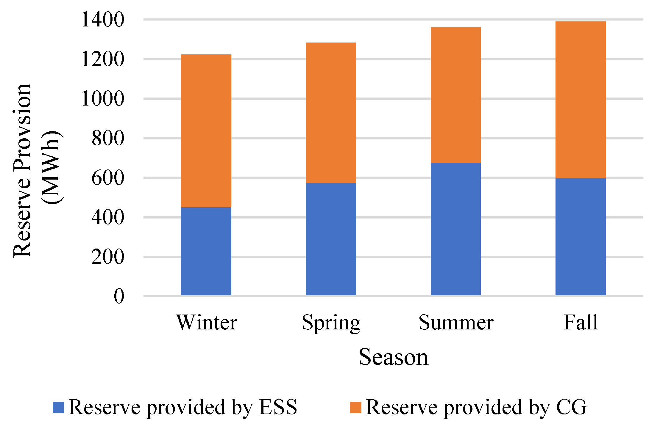
It is worth noting that the ESS, in addition to CG, could result in a higher ESS sizing and hence a higher investment cost by providing the reserve to meet the reserve requirement. Figure 10 shows the seasonal reserve provided by the ESS and CG. It can be noted that the ESS provided a substantial percentage of the reserve.
4. Conclusions
A mixed integer linear programming (MILP) model for optimal sizing of energy storage for islanded microgrids was presented. The model is a unit commitment model and considers the following: unavailability of solar cell generators, seasonal correlation of solar radiation with demand, operational constraints of CG, and demand and reserve requirements. When running the proposed model, we showed that the ESS sizing, when considering Li-Ion technology and an SCG penetration of 25%, was on average approximately 3 MWh and 1.7 MW. The case study also showed that the CG cost was significantly reduced in the presence of ESS when compared to a scenario without ESS. This reduction could be attributed to a change in the operation of CG when an ESS was present, resulting in lower costs.
While this model considers several aspects, it has some limitations that could be addressed in future work. These include ESS degradation over time, in addition to factors that affect SCG efficiency. In future work, we intend to use the proposed approach for more accurate modeling of long-term ESS operation. The effect of SCG derating factors, such as soiling, conversion, temperature-related factors, and others affecting ESS sizing, are also important and will be considered in future work.
Author Contributions
Conceptualization, A.A. (Abdullah Alamri); methodology, A.A. (Abdullah Alamri); software, A.A. (Abdullah Alamri); validation, A.A. (Abdullah Alamri) and A.A. (Abdulrahman AlKassem); formal analysis, A.A. (Abdullah Alamri); investigation, A.A. (Abdullah Alamri) and A.D.; resources, A.A. (Abdullah Alamri) and A.D.; data curation, A.A. (Abdulrahman AlKassem); writing—original draft preparation, A.A. (Abdullah Alamri); writing—review and editing, A.A. (Abdullah Alamri), A.D. and A.A. (Abdulrahman AlKassem); visualization, A.A. (Abdullah Alamri) and A.A. (Abdulrahman AlKassem); supervision, A.A. (Abdullah Alamri) and A.D.; project administration, A.A. (Abdullah Alamri) and A.A. (Abdulrahman AlKassem); funding acquisition, A.D. All authors have read and agreed to the published version of the manuscript.
Funding
The research was funded by the Islamic University of Madinah (IUM) in Saudi Arabia through the Deanship of Scientific Research (DSR) under grant no. 656 in November 2020 through the “Tamayyuz 2” Financial Program.
Institutional Review Board Statement
Not applicable.
Informed Consent Statement
Not applicable.
Data Availability Statement
Not applicable.
Conflicts of Interest
The authors declare no conflict of interest.
References
- IEEE Std 2030.7-2017; IEEE Standard for the Specification of Microgrid Controllers. IEEE: New York, NY, USA, 2018; pp. 1–43.
- Choudhury, S. A comprehensive review on issues, investigations, control and protection trends, technical challenges and future directions for Microgrid technology. Int. Trans. Electr. Energy Syst. 2020, 30, e12446. [Google Scholar] [CrossRef]
- The, U.S. Energy Information Administration (EIA). U.S. Battery Storage Market Trends; The U.S. Energy Information Administration (EIA): Washington, DC, USA, 2018. [Google Scholar]
- Parhizi, S.; Lotfi, H.; Khodaei, A.; Bahramirad, S. State of the Art in Research on Microgrids: A Review. IEEE Access 2015, 3, 890–925. [Google Scholar] [CrossRef]
- Ghiassi-Farrokhfal, Y.; Rosenberg, C.; Keshav, S.; Adjaho, M.-B. Joint Optimal Design and Operation of Hybrid Energy Storage Systems. IEEE J. Sel. Areas Commun. 2016, 34, 639–650. [Google Scholar] [CrossRef] [Green Version]
- Dong, J.; Gao, F.; Guan, X.; Zhai, Q.; Wu, J. Storage Sizing with Peak-Shaving Policy for Wind Farm Based on Cyclic Markov Chain Model. IEEE Trans. Sustain. Energy 2016, 8, 978–989. [Google Scholar] [CrossRef]
- Arabali, A.; Ghofrani, M.; Etezadi-Amoli, M.; Fadali, M.S. Stochastic Performance Assessment and Sizing for a Hybrid Power System of Solar/Wind/Energy Storage. IEEE Trans. Sustain. Energy 2013, 5, 363–371. [Google Scholar] [CrossRef]
- Alamri, A.; AlOwaifeer, M.; Meliopoulos, A.S.; Cokkinides, G.J. Energy Storage Sizing and Reliability Assessment for Power Systems with Variable Generation. In Proceedings of the 2019 IEEE Milan PowerTech, Milano, Italy, 23–27 June 2019; pp. 1–6. [Google Scholar] [CrossRef]
- Alamri, A.; Alowaifeer, M.; Meliopoulos, A.P.S. Energy Storage Sizing and Probabilistic Reliability Assessment for Power Systems Based on Composite Demand. IEEE Trans. Power Syst. 2021, 37, 106–117. [Google Scholar] [CrossRef]
- Zhang, Y.; Wang, J.; Berizzi, A.; Cao, X. Life cycle planning of battery energy storage system in off-grid wind_solar_diesel microgrid. IET Gener. Transmiss. Distrib. 2018, 12, 4451–4461. [Google Scholar] [CrossRef]
- Zolfaghari, M.; Ghaffarzadeh, N.; Ardakani, A.J. Optimal sizing of battery energy storage systems in off-grid micro grids using convex optimization. J. Energy Storage 2019, 23, 44–56. [Google Scholar] [CrossRef]
- Hesaroor, K.; Das, D. Optimal sizing of energy storage system in islanded microgrid using incremental cost approach. J. Energy Storage 2019, 24, 100768. [Google Scholar] [CrossRef]
- Pham, C.M.; Tran, Q.T.; Bacha, S.; Hably, A.; Nugoc, A.L. Optimal sizing of battery energy storage system for an island microgrid. In Proceedings of the IECON 2018—44th Annual Conference of the IEEE Industrial Electronics Society, Washington, DC, USA, 21–23 October 2018. [Google Scholar]
- Bahramirad, S.; Reder, W.; Khodaei, A. Reliability-Constrained Optimal Sizing of Energy Storage System in a Microgrid. IEEE Trans. Smart Grid 2012, 3, 2056–2062. [Google Scholar] [CrossRef]
- Zhu, W.; Guo, J.; Zhao, G.; Zeng, B. Optimal Sizing of an Island Hybrid Microgrid Based on Improved Multi-Objective Grey Wolf Optimizer. Processes 2020, 8, 1581. [Google Scholar] [CrossRef]
- Cao, B.; Dong, W.; Lv, Z.; Gu, Y.; Singh, S.; Kumar, P. Hybrid Microgrid Many-Objective Sizing Optimization With Fuzzy Decision. IEEE Trans. Fuzzy Syst. 2020, 28, 2702–2710. [Google Scholar] [CrossRef]
- Bandyopadhyay, S.; Mouli, G.R.C.; Qin, Z.; Elizondo, L.R.; Bauer, P. Techno-Economical Model Based Optimal Sizing of PV-Battery Systems for Microgrids. IEEE Trans. Sustain. Energy 2019, 11, 1657–1668. [Google Scholar] [CrossRef]
- Ropero-Castaño, W.; Muñoz-Galeano, N.; Caicedo-Bravo, E.F.; Maya-Duque, P.; López-Lezama, J.M. Sizing Assessment of Islanded Microgrids Considering Total Investment Cost and Tax Benefits in Colombia. Energies 2022, 15, 5161. [Google Scholar] [CrossRef]
- Park, J.; Liang, W.; Choi, J.; El-Keib, A.A.; Shahidehpour, M.; Billinton, R. A probabilistic reliability evaluation of a power system including Solar/Photovoltaic cell generator. In Proceedings of the 2009 IEEE Power & Energy Society General Meeting, Calgary, AB, Canada, 26–30 July 2009; pp. 1–6. [Google Scholar] [CrossRef]
- Allan, R.; Billinton, R. Reliability Evaluation of Power Systems, 1st ed.; Plenum: New York, NY, USA, 1996. [Google Scholar]
- Ostrowski, J.; Anjos, M.F.; Vannelli, A. Tight Mixed Integer Linear Programming Formulations for the Unit Commitment Problem. IEEE Trans. Power Syst. 2011, 27, 39–46. [Google Scholar] [CrossRef]
- Atakan, S.; Lulli, G.; Sen, S. A State Transition MIP Formulation for the Unit Commitment Problem. IEEE Trans. Power Syst. 2017, 33, 736–748. [Google Scholar] [CrossRef] [Green Version]
- Baker, K.; Hug, G.; Li, X. Energy Storage Sizing Taking into Account Forecast Uncertainties and Receding Horizon Operation. IEEE Trans. Sustain. Energy 2016, 8, 331–340. [Google Scholar] [CrossRef]
- Zimmerman, R.D.; Murillo-Sanchez, C.; Thomas, R.J. MATPOWER’s extensible optimal power flow architecture. In Proceedings of the 2009 IEEE Power & Energy Society General Meeting, Calgary, AB, Canada, 26–30 July 2009; pp. 1–7. [Google Scholar]
- Wood, A.J.; Wollenberg, B.F. Power Generation, Operation, and Control, 2nd ed.; Wiley: New York, NY, USA, 1996. [Google Scholar]
- Carrion, M.; Arroyo, J. A Computationally Efficient Mixed-Integer Linear Formulation for the Thermal Unit Commitment Problem. IEEE Trans. Power Syst. 2006, 21, 1371–1378. [Google Scholar] [CrossRef]
- Renewable Resource Atlas, King Abdullah City for Atomic and Renewable Energy (K.A.CARE). Available online: https://www.energy.gov.sa/en/projects/Pages/atlas.aspx (accessed on 23 August 2022).
- Open Energy Data Initiative (OEDI). The U.S. Department of Energy (DOE). Available online: https://data.openei.org (accessed on 20 September 2022).
- Bahramirad, S.; Camm, E. Practical modeling of Smart Grid SMS storage management system in a microgrid. In Proceedings of the PES T&D 2012, Orlando, FL, USA, 7–10 May 2012; pp. 1–7. [Google Scholar] [CrossRef]
- NREL System Advisor Model (SAM). Available online: https://sam.nrel.gov (accessed on 12 June 2022).
- Spertino, F.; Chiodo, E.; Ciocia, A.; Malgaroli, G.; Ratclif, A. Maintenance Activity, Reliability, Availability, and Related Energy Losses in Ten Operating Photovoltaic Systems up to 1.8 MW. IEEE Trans. Ind. Appl. 2020, 57, 83–93. [Google Scholar] [CrossRef]
- Schoenung, S. Energy Storage Systems Cost Update: A Study for the DOE Energy Storage Systems Program; Department of Energy: USA, 2011. [Google Scholar] [CrossRef]
Figure 1.
Flowchart of the proposed model.
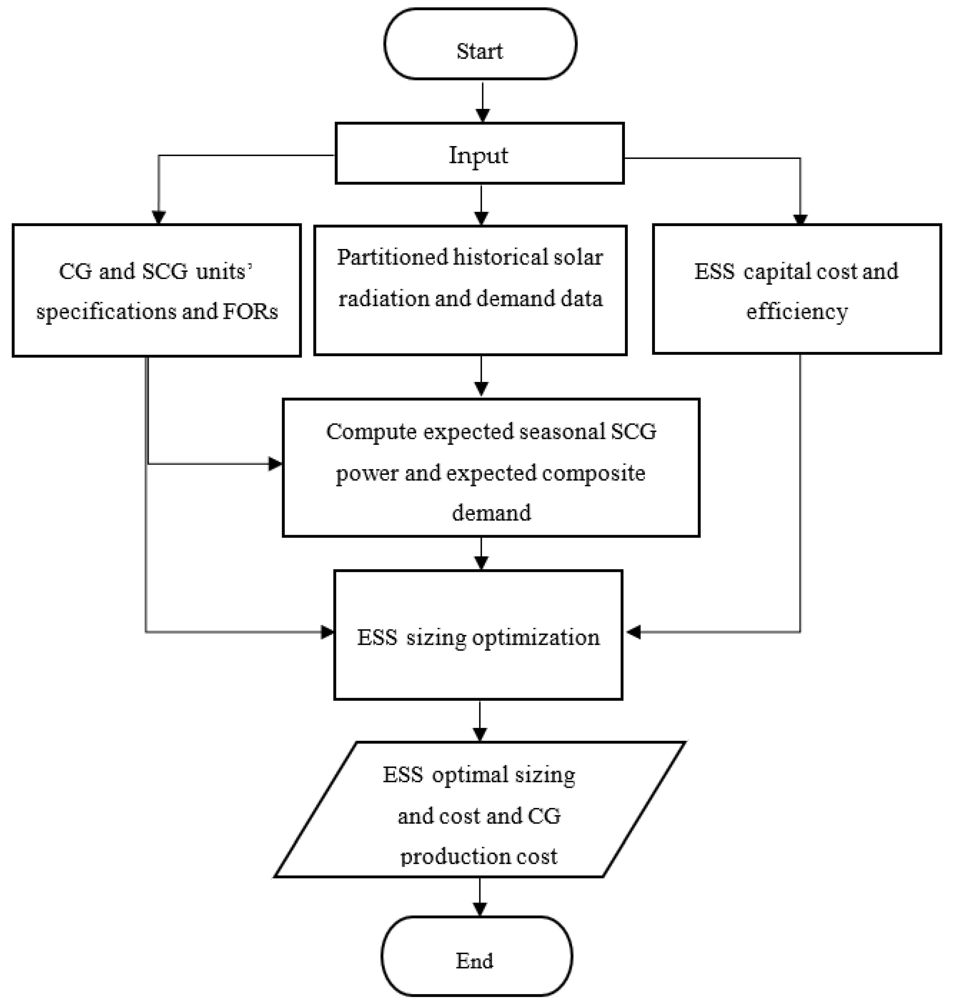
Figure 2.
SCG availability model.
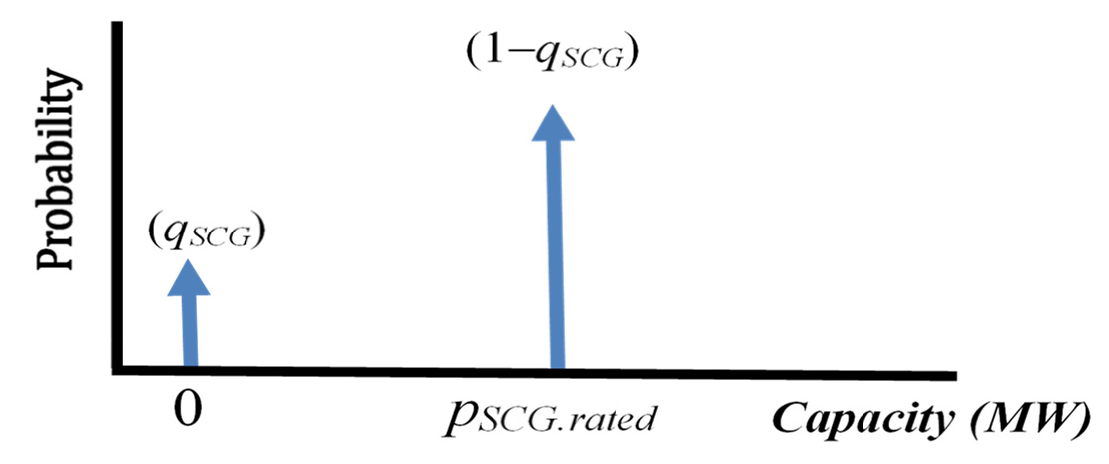
Figure 3.
SCG output probability tree.

Figure 4.
SF availability PMF (ρSFA(cSF)).
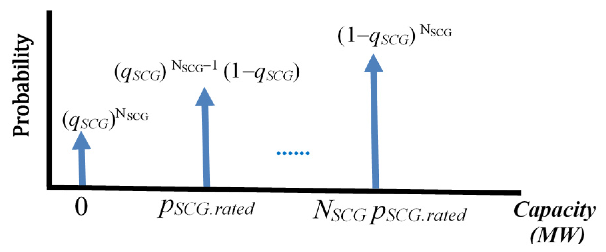
Figure 5.
Solar radiation seasonal samples.
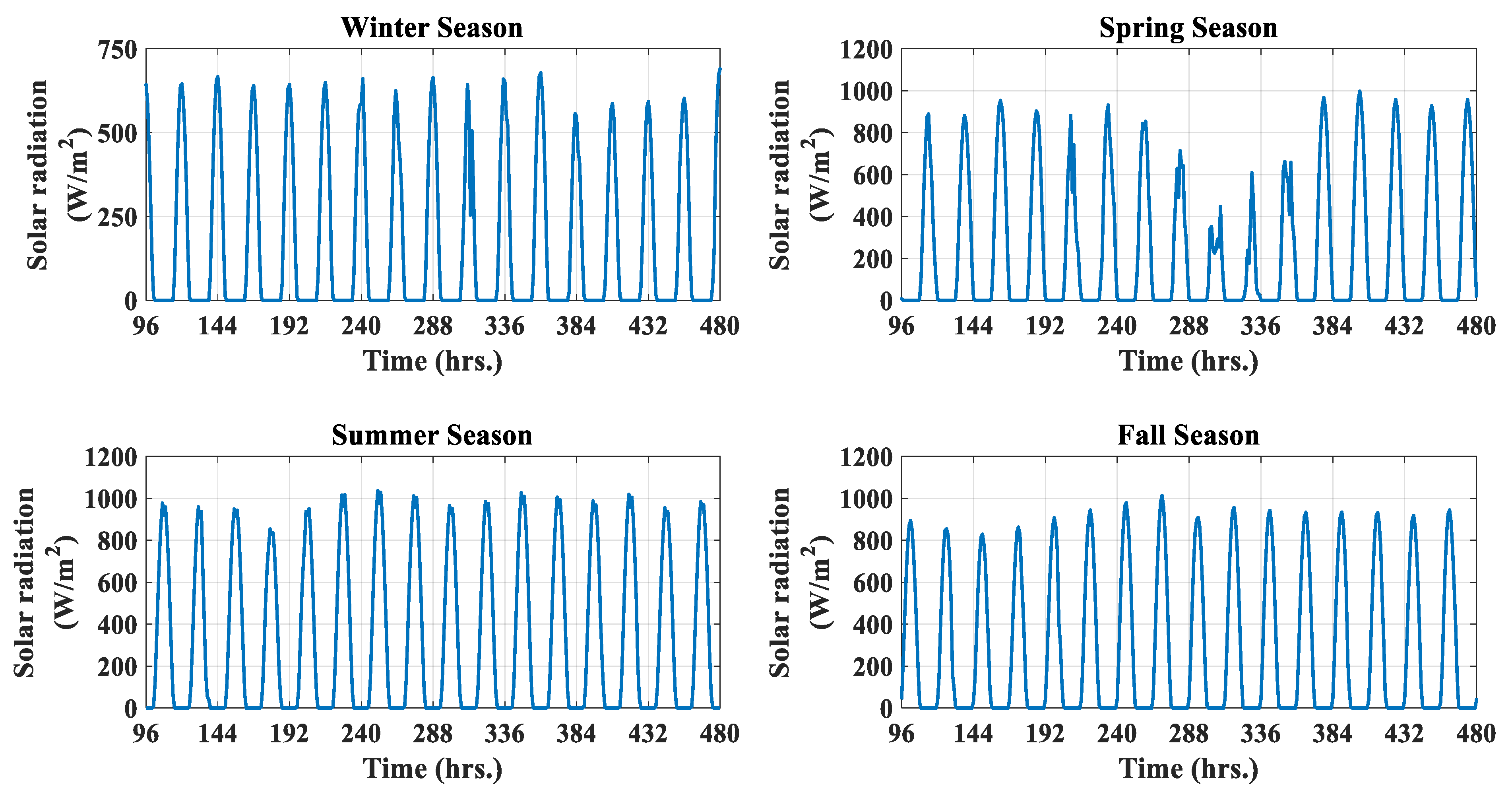
Figure 6.
Expected seasonal power output of SF.
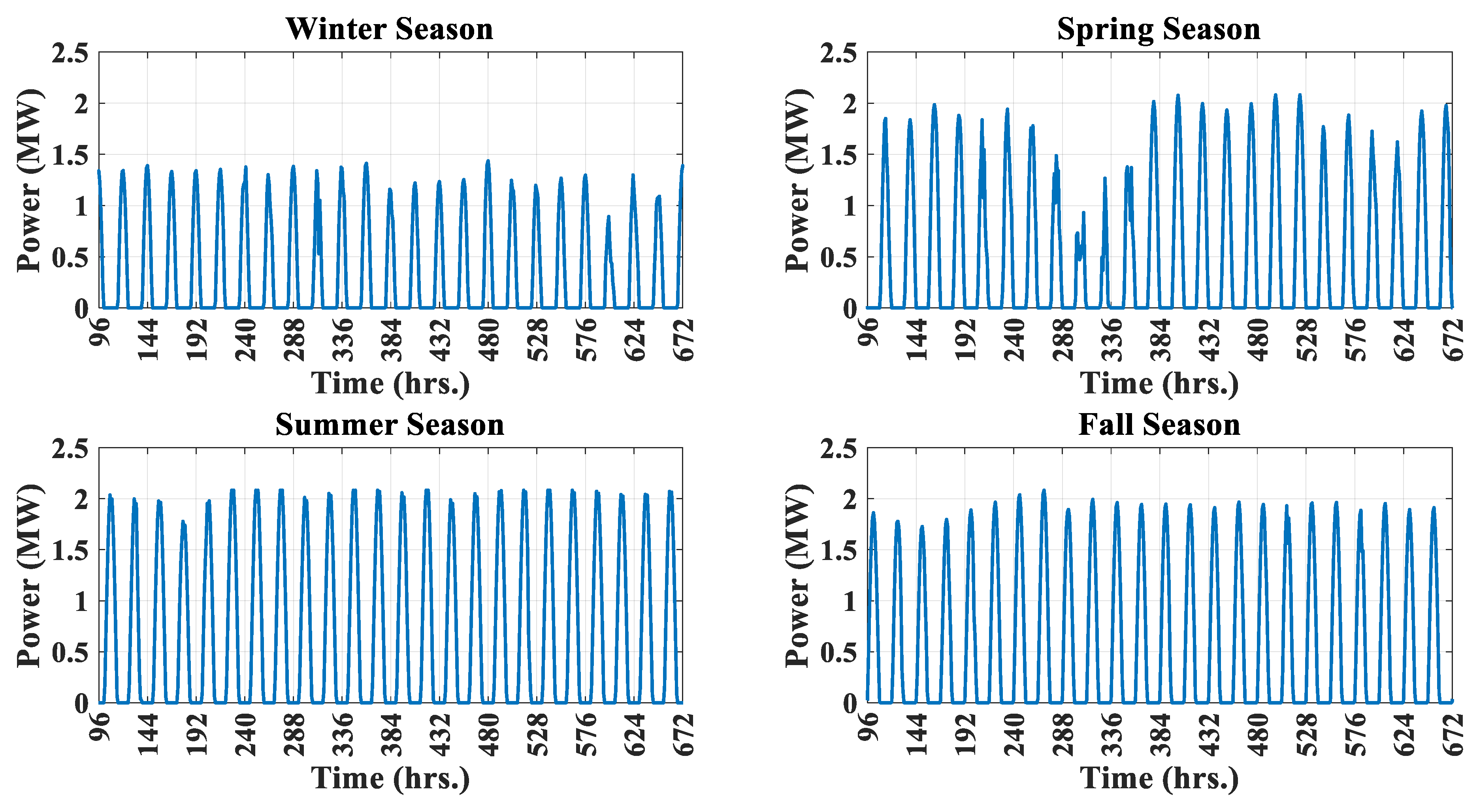
Figure 7.
Seasonal expected composite demand.

Figure 8.
Seasonal variations of ρCD (cd).
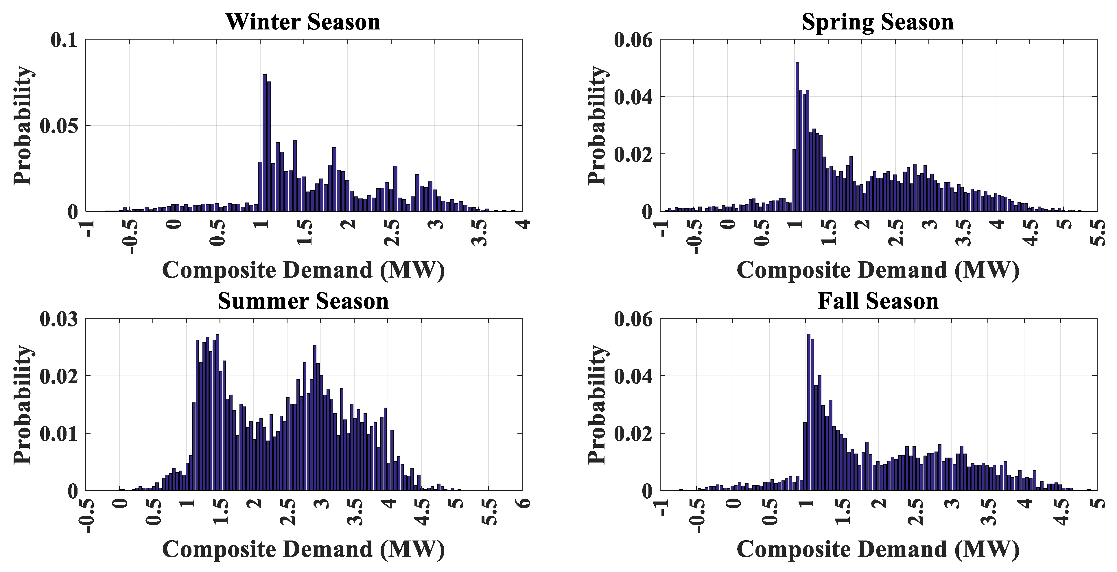
Figure 9.
Seasonal variation of the ESS SOC.
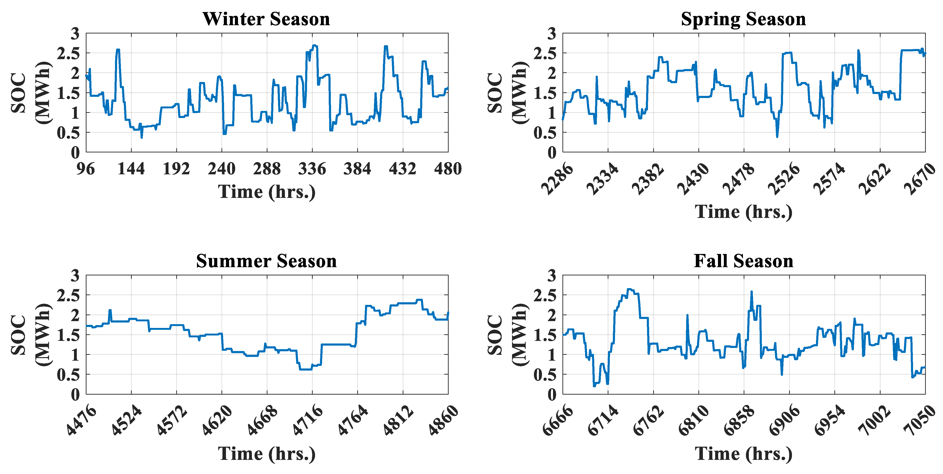
Figure 10.
Seasonal reserve provision by the ESS and CG.

Table 1.
Variables and parameters used in the model.
| Parameter/Variable | Description (unit) |
|---|---|
| Parameters and variables for CG units: | |
| CTg | Cold start time (h) |
| DTg/UTg | Minimum down/up times of a CG (h) |
| SUg/SDg | Startup/shutdown limit of a CG (MWh−1) |
| SUcost/SDcost | gth CG linearized startup/shutdown costs |
| sg,t | Binary variable of the gth CG startup status (1: turned on, 0: shut down) |
| rg,t | gth CG reserve provision (MW) |
| RUg/RDg | Ramp-up/down rates of a CG (MW) |
| Maximum/minimum generation limits of a CG (MW) | |
| pg,t is | gth CG produced power (MW) |
| gth CG provided power and reserve (MW) | |
| xg,t | Binary variable of the gth CG status (0: off, 1: on) |
| yg,t | gth CG linearized production cost |
| zg,t | Binary variable of the gth CG shutdown status (1: turned off, 0: otherwise) |
| Parameters and variables for ESS: | |
| αt | Binary variable to prevent ESS’s simultaneous charging and discharging |
| d | ESS energy capacity capital cost ($/MWh) |
| e | ESS power capacity capital cost ($/MW) |
| EESS | Energy capacity of ESS (MWh) |
| Et | ESS energy level or state of charge at time t |
| ηch/ηdis | Charging/discharging efficiency |
| rESS_DN,t | Down reserve provided by the ESS (MW) |
| rESS_UP,t | Up reserve provided by the ESS (MW) |
| R | Reserve requirement (MW) |
| pch,t | Power charging of ESS (MW) |
| pdis,t | Power discharging from ESS (MW) |
| PESS | Maximum discharge/charge rate of ESS (MW) |
| ESS charging power and down reserve (MW) | |
| ESS discharging power and up reserve (MW) | |
Table 2.
CG units’ characteristics [29].
Table 2.
CG units’ characteristics [29].
| Unit | Cost Coeff. ($/MWh) | Min. Capacity (MW) | Max. Capacity (MW) | Startup Cost ($) |
| 1 | 27.7 | 1 | 5 | 40 |
| 2 | 39.1 | 1 | 5 | 40 |
| Unit | Shutdown Cost ($) | Min. Up Time (h) | Min. Down Time (MW) | Ramp Up/Down Rate (MW/h) |
| 1 | 0 | 3 | 3 | 2.5 |
| 2 | 0 | 3 | 3 | 2.5 |
| Specification | Description |
|---|---|
| pSCG.rated | 0.05 MW |
| NSCG | 50 |
| Gstd | 1000 W/m2 |
| RC | 150 W/m2 |
| qSCG | 0.1667 |
| MTTFSCG | 1500 h. |
| MTTRSCG | 150 h. |
Table 4.
CG units’ characteristics [32].
Table 4.
CG units’ characteristics [32].
| Specification | Description |
|---|---|
| ESS technology | Li-Ion |
| ηch/ηdis | 85% |
| Energy capital cost | 600k $/MWh |
| Power capital cost | 400k $/MW |
| Lifetime | 20 years |
| Discount rate | 5% |
| e | 51,814 $/MW |
| d | 77,720 $/MWh |
Table 5.
Demand data [28].
Table 5.
Demand data [28].
| Demand Type | Average (KWh/Day) | Average (KW) | Peak (KW) | Demand Factor | #Units |
|---|---|---|---|---|---|
| Secondary school | 10,086 | 420.25 | 1212.2 | 0.35 | 1 |
| Primary school | 2656 | 110.67 | 371.78 | 0.3 | 1 |
| Midrise apartment building | 749.81 | 31.24 | 73.64 | 0.42 | 20 |
| Medium office | 2022.5 | 84.27 | 254.42 | 0.33 | 1 |
| Outpatient clinic | 3956.2 | 164.84 | 360.77 | 0.46 | 1 |
| Fast food restaurant | 560.48 | 23.35 | 41.78 | 0.56 | 5 |
| Large office | 17,831 | 742.99 | 1531 | 0.49 | 1 |
| Independent retailer | 923.9 | 38.5 | 104.83 | 0.37 | 5 |
Table 6.
ESS sizing and CG operational cost results.
| Case | EESS (MWh) | PESS (MW) | Total Cost ($) | ESS Cost ($) | CG Cost ($) |
|---|---|---|---|---|---|
| CG and PV (no ESS) | NA | NA | 718,638 ± 1042 | NA | 718,638 ± 1042 |
| CG and PV+ESS | 3.0 ± 0.30 | 1.70 ± 0.40 | 815,465 ± 22,259 | 320,514 ± 34,950 | 494,951 ± 20,857 |
Disclaimer/Publisher’s Note: The statements, opinions and data contained in all publications are solely those of the individual author(s) and contributor(s) and not of MDPI and/or the editor(s). MDPI and/or the editor(s) disclaim responsibility for any injury to people or property resulting from any ideas, methods, instructions or products referred to in the content. |
© 2023 by the authors. Licensee MDPI, Basel, Switzerland. This article is an open access article distributed under the terms and conditions of the Creative Commons Attribution (CC BY) license (https://creativecommons.org/licenses/by/4.0/).
Share and Cite
MDPI and ACS Style
Alamri, A.; AlKassem, A.; Draou, A. Composite Demand-Based Energy Storage Sizing for an Isolated Microgrid System. Sustainability 2023, 15, 1517. https://doi.org/10.3390/su15021517
AMA Style
Alamri A, AlKassem A, Draou A. Composite Demand-Based Energy Storage Sizing for an Isolated Microgrid System. Sustainability. 2023; 15(2):1517. https://doi.org/10.3390/su15021517
Chicago/Turabian StyleAlamri, Abdullah, Abdulrahman AlKassem, and Azeddine Draou. 2023. "Composite Demand-Based Energy Storage Sizing for an Isolated Microgrid System" Sustainability 15, no. 2: 1517. https://doi.org/10.3390/su15021517
Note that from the first issue of 2016, this journal uses article numbers instead of page numbers. See further details here.