Predicting the Compressive Strength of Green Concrete at Various Temperature Ranges Using Different Soft Computing Techniques

Abstract

To overcome the environmental impact of cement production in concrete, the construction industry is adopting eco-friendly approaches, such as incorporating alternative and recycled materials and minimizing carbon emissions in concrete production. One such material that has gained prominence is ground granulated blast furnace slag (GGBFS). This study focuses on investigating the compressive strength of concrete at 28 days of age by examining the influences of several factors, such as temperature, water-to-binder ratio (w/b), GGBFS-to-binder ratio (GGBFS/b), fine aggregate, coarse aggregate, and superplasticizer. A statistical modeling approach was employed to comprehensively analyze these parameters and assess their impact on compressive strength. To accomplish this, the study collected and analyzed data from the literature, resulting in a dataset of 210 observations. The dataset was divided into training and testing groups, and statistical analyses were performed to assess the relationships between the input parameters and compressive strength. The correlation analysis revealed insignificant relationships between the input parameters and compressive strength, indicating that multiple factors affect strength. Different models were employed to predict compressive strength, such as linear regression, nonlinear regression, quadratic, full quadratic models, and artificial neural networks (ANN). The findings of this study contribute to a better understanding of the factors that influence the compressive strength of concrete containing GGBFS. The results underscore the importance of considering multiple parameters to predict strength accurately.

1. Introduction

In the construction sector, sustainability has emerged as a crucial concern, and concrete, one of the most commonly used building materials, has a substantial environmental impact. In addition to other environmental effects, including increased waste creation, concrete production is a major contributor to the world’s greenhouse gas emissions. In order to solve these problems, the concrete industry is placing an increasing amount of emphasis on environmentally friendly methods of production and advancements in concrete constructions’ long-term durability. This entails the utilization of alternative and recycled materials, creating concrete mixtures with minimal carbon emissions, and applying sustainable design concepts to concrete construction.

The construction industry has placed greater emphasis on sustainability as engineering firms and government agencies aim to reduce the environmental impact of building projects. A variety of factors drive the usage of mineral admixtures in construction. These include economic considerations, such as the desire to reduce cement requirements, minimizing energy usage and environmental concerns [1]. Additionally, incorporating mineral admixtures is motivated by improving concrete’s engineering and performance properties [1]. Reducing the amount of cement required in concrete also decreases the carbon dioxide emissions produced during cement production [2,3,4,5]. Ground granulated blast furnace slag (GGBFS) has emerged as a crucial material in promoting sustainability in concrete construction. Utilizing industrial byproducts such as GGBFS has been shown to enhance concrete’s mechanical characteristics and longevity. This practice also contributes to reducing CO₂ emissions, conserving energy, and alleviating the negative environmental impacts associated with concrete production [6].

The qualities of concrete, such as its workability, strength, and durability, are improved when GGBFS, a byproduct of the iron industry, is added. This substance is produced when iron ore, limestone, and coke are heated to roughly 1500 degrees Celsius [7]. GGBFS does not directly come into being. Both molten slag and molten iron are byproducts of the production of iron. Ca(O), SiO₂, AL₂ O, and MgO are the primary ingredients in blast furnace slag. In the majority of cementitious materials, these minerals are present. Ground granulated blast furnace slag cement is further dried, and the particles are ground in a spinning ball mill to create a fine powder [7]. Blast furnace slag is a byproduct generated during the iron production process in a blast furnace. By rapidly cooling and finely grinding molten slag into a cement-like form, it becomes known as GGBFS (ground granulated blast furnace slag). The use of ground granulated blast furnace slag (GGBFS) can contribute to environmental sustainability in several ways. GGBFS is a byproduct of the iron and steel industry, obtained by quenching molten slag from a blast furnace with water or steam. The following are some ways GGBFS promotes environmental sustainability. Reduced carbon emissions: GGBFS can replace a portion of cement in concrete production. Cement production is a significant source of carbon dioxide (CO₂) emissions due to the calcination process and the use of fossil fuels. By substituting cement with GGBFS, the overall carbon footprint of concrete can be reduced. GGBFS has a lower embodied carbon than cement, helping mitigate greenhouse gas emissions. Energy conservation: The production of GGBFS requires less energy than does cement production. Blast furnace slag is a byproduct that would otherwise be discarded, so using it as a cementitious material reduces the need for energy-intensive processes associated with cement production, such as limestone quarrying and clinker grinding. This form of energy conservation contributes to environmental sustainability by reducing energy consumption and the associated greenhouse gas emissions. Waste reduction: GGBFS utilizes waste material that would otherwise be disposed of in landfills. Incorporating blast furnace slag into concrete prevents the accumulation of this waste material and reduces the need for landfills, promoting sustainable waste management practices. Improved durability: Concrete containing GGBFS generally exhibits enhanced durability compared to that of conventional concrete. GGBFS contributes to reducing the permeability of concrete, making it more resistant to chloride penetration, sulfate attack, and alkali–aggregate reactions. This increased durability leads to a longer service life for concrete structures, reducing the need for frequent repairs and replacements. Consequently, using GGBFS helps conserve resources and minimize the environmental impact associated with construction and demolition activities. Reduced water consumption: GGBFS concrete typically has a slower hydration process than traditional cement does. This slower hydration allows for better workability and extended setting times, reducing the need for excessive water use during concrete placement. GGBFS contributes to water conservation and sustainable water management practices by minimizing water requirements. Overall, GGBFS offers various environmental benefits, including reduced carbon emissions, energy conservation, waste reduction, improved durability, and reduced water consumption. By incorporating GGBFS into construction materials, we can contribute to a more sustainable and environmentally friendly built environment [8].

GGBFS, functioning as a latent hydraulic material, reacts with calcium hydroxide (Ca (OH)₂) and water, resulting in the formation of calcium silicate hydrate (C-S-H). This C-S-H compound plays a crucial role in determining the strength of cement-based materials [8,9]. Through a pozzolanic reaction, incorporating GGBFS as a supplementary cementitious material can decrease early strength while enhancing ultimate strength. Moreover, it substantially positively impacts the microstructure and durability of hardened concrete [10,11]. The ASTM C989 slag activity index serves as a crucial benchmark for comparatively evaluating the cementitious capacity of slag cement [12,13,14]. The categorization of slag into three grades (80, 100, and 120) is determined based on the strength of mortars produced by blending the slag with Portland cement in equal proportions, in accordance with the provisions of ASTM C989 [15,16,17]. The slag consists of lime, silica, and alumina. The same oxides are found in Portland cement, although they are not present in the same proportions [18,19]. This paper explores the impact of GGBFS with varying replacement levels, supplemented with superplasticizer, on the mechanical properties of concrete under different curing temperature conditions ranging from 5 °C to 75 °C. The study also investigates the mechanical properties of GGBFS, specifically within the range of 0.25 to 0.889 of the water-to-binder ratio and within the range of 0 to 2.9% of superplasticizer content. Furthermore, this study examines the effect of various factors, including fine aggregate content, coarse aggregate content, superplasticizer dosage, and curing time at 28 days, on the compressive strength of concrete enhanced with a superplasticizer.

Multiple model techniques were employed to predict the compressive strength of concrete, namely linear, nonlinear, quadratic, full quadratic, and artificial neural networks. These models were trained using a comprehensive dataset comprising 210 records from relevant literature sources [8,9,20,21,22,23,24,25,26,27,28,29,30]. Compressive strength is a significant indicator of the mechanical properties of GGBFS as a cement substitute. The performance of the models was evaluated using statistical criteria such as R² (coefficient of determination), RMSE (root mean squared error), and MAE (mean absolute error). Numerical techniques were employed to develop a model capable of estimating the compressive strength of concrete incorporating a superplasticizer. The models considered six parameters as input data: temperature, water-to-binder ratio, GGBFS-to-binder ratio, fine aggregate content, coarse aggregate content, and curing time at 28 days, along with the superplasticizer dosage. A comprehensive database comprising 210 records from various literature sources was compiled to train and test each of the five models.

2. Research Objective

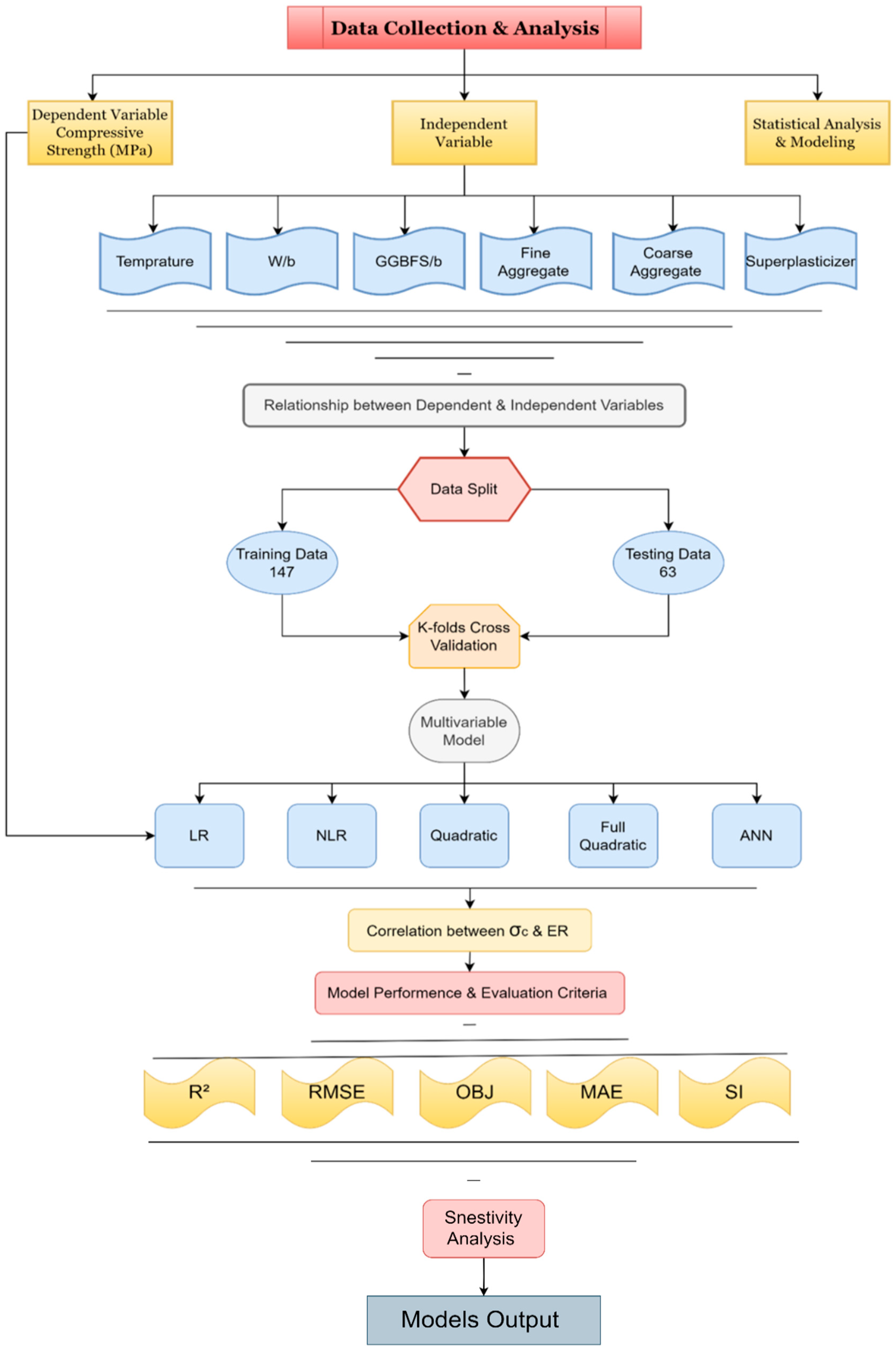
The main objective of this study is to investigate the compressive strength of concrete at 28 days of age by adjusting several variables, such as temperature, water-to-binder ratio, GGBFS-to-binder ratio, fine aggregate, coarse aggregate, and superplasticizer content. Several multiscale models were used to analyze data from previous research investigations to achieve this goal. Furthermore, the influence of ground granulated blast furnace slag (GGBFS) on the compressive strength of concrete was investigated and the optimal model with the lowest RMSE to measure the compressive strength of concrete containing GGBFS was identified.

3. Methodology

The data set used in this study was acquired from several research papers consisting of 210 observations. The data were subjected to statistical analysis to better understand the data set. The dataset was then divided into two groups; the first group consisted of 147 observations, representing 70% of the total dataset. This set was used as training data to develop a predictive model. The second group contained 63 observations, representing 30% of the data set, and was used as testing data to evaluate the performance and accuracy of the developed prediction models.

Table 1. The Summary of the database utilized during the modeling procedure.

Reference	No. of Data	Temperature °C	w/b (%)	GGBFS/b (%)	FA (kg/m3)	CA (kg/m3)	Time (Days)	SP (%)	CS (MPa)
[8]	25	20	0.442–0.889	0–0.61	526–748	799–1135	28	0	18.1–47.5
[26]	7	20	0.27–0.42	0–0.5	608–780	965–981	28	0.413–1.52	44.6–71.4
[27]	11	20	0.27–0.445	0–0.5	608–783	923–981	28	0.15–1.52	44.6–71.4
[28]	2	20	0.56	0.55, 0.58	750	1080	28	0	33.5,42,5
[29]	4	20	0.41	0–0.5	697	1035	28	2.9	46.4–48.3
[30]	161	5–75	0.25–0.756	0–0.7	395–947	863–1080	28	0–2.04	17.2–72.4
Remarks	210	Ranged between 5–75	Ranged between	Ranged between	Ranged between	Ranged between	Ranged between	Ranged between	Ranged between
			0.25–0.889	0–0.7	395–947	799–1135	28	0–2.9	17.2–72.4

provides an overview of the data used in both the training and testing datasets. The research study methodology and the steps taken in data collection, analysis, and model development are shown in Figure 1, which illustrates the research flow chart. Various mathematical and statistical techniques were used to show the correlation of fundamental characteristics between the input and output parameters. By observing the interaction between these variables, a comprehensive understanding of the underlying processes was achieved, and a more accurate model was developed. The parameters evaluated were temperature, w/b, GGBFS/b, and fine aggregate, coarse aggregate, and superplasticizer content. A marginal plot was generated for each parameter to investigate the relationship between each parameter and compressive strength, as shown in Figure 2. Furthermore, compressive strength (σc) and each parameter were analyzed using standard deviation (SD), variance (Var), skewness (Skew), and kurtosis (Kur).

4. Statistical Analysis

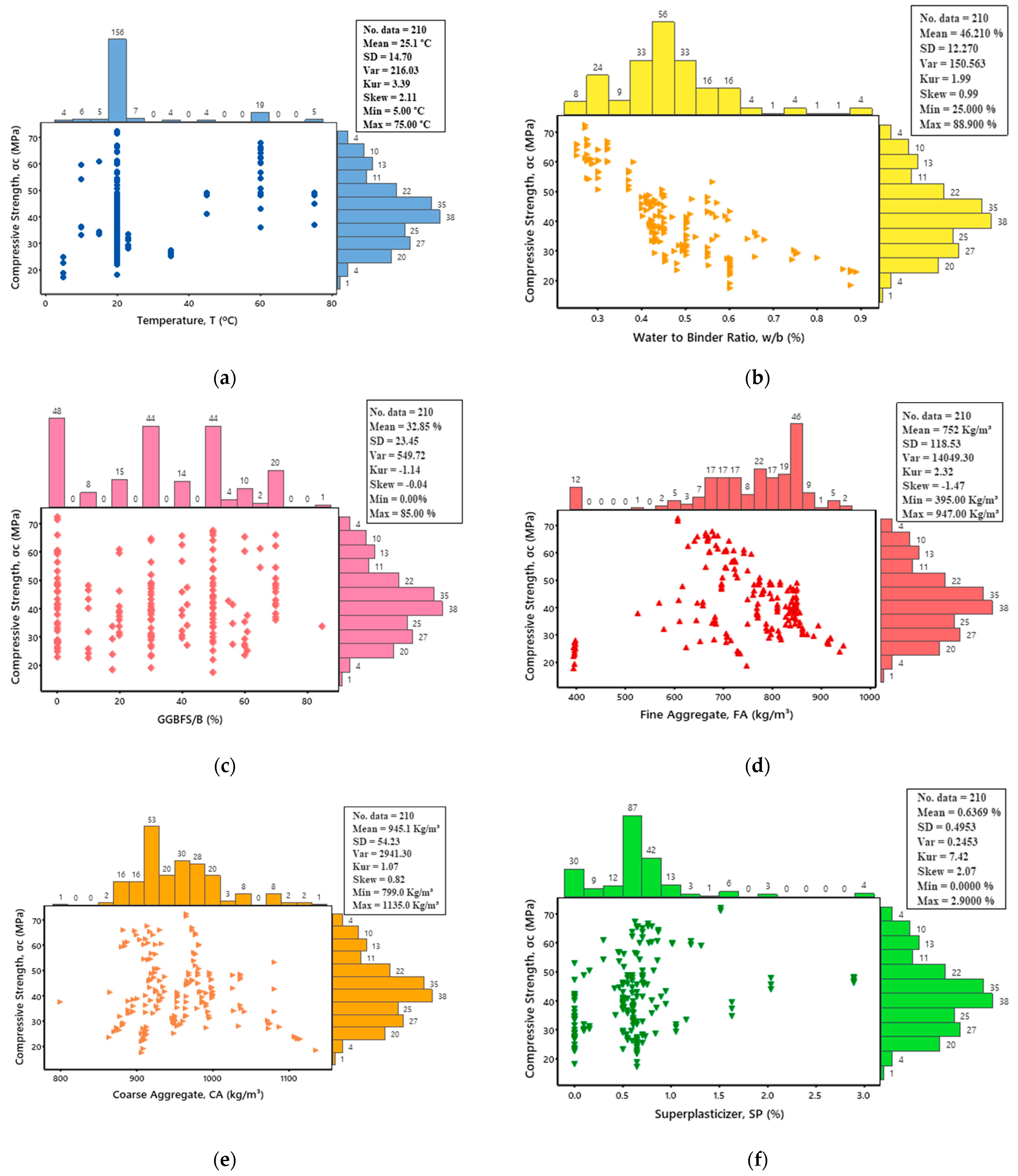
4.1. Temperature

In Figure 2a, a comprehensive analysis is provided regarding the correlation between compressive strength and temperature (T). The temperature range varied between 5.00 and 75.00 °C, with a clear representation of minimum and maximum values. Additionally, the statistical measures of mean and standard deviation were determined to be 25.1 °C and 14.70, respectively, while the variance was 216.03. These values were further complemented with the kurtosis and skewness values of 3.39 and 2.11, respectively, providing a more in-depth understanding of the relationship between compressive strength and temperature.

4.2. Water-to-Binder Ratio (w/b)

Figure 2b examines the connection between compressive strength and water-to-binder ratio (w/b). The w/b values were measured, ranging from 25 to 88.90%, highlighting the minimum and maximum values. Moreover, the statistical analysis revealed the mean and standard deviation to be 46.210% and 12.27, respectively, while the variance was calculated to be 150.56. These findings were further reinforced by the kurtosis and skewness values of 1.99 and 0.99, respectively, providing an in-depth comprehension of the relationship between compressive strength and w/b.

4.3. GGBFS to the Binder Ratio

Figure 2c investigates the correlation between compressive strength and the GGBFS-to-binder ratio (GGBFS/b), with variations in GGBFS/b values ranging from 0.00 to 85.00%. The range encompasses the minimum and maximum values. A statistical analysis of the data revealed that the mean and standard deviation were 32.85% and 23.45%, respectively, while the variance was calculated to be 549.72. These results were further strengthened by the kurtosis and skewness values of −1.14 and −0.04, respectively, which provide an in-depth understanding of the relationship between compressive strength and GGBFS/b.

4.4. Fine Aggregate

Figure 2e presents a comprehensive analysis that examines the correlation between fine aggregate (FA) and compressive strength. The FA range used in the analysis was between 395.00 and 947.00 kg/m³ for the minimum and maximum values. The analysis further determined statistical measures such as mean and standard deviation, which were 752.00 kg/m³ and 118.53, respectively. The variance was 14,049.30. Moreover, kurtosis and skewness values of 2.32 and −1.47 were obtained, providing a more detailed understanding of the relationship between compressive strength and FA.

4.5. Coarse Aggregate

A detailed analysis of the correlation between coarse aggregate (CA) and compressive strength is depicted in Figure 2f. The analysis employed a CA range of 799.00 to 1135.00 kg/m³, effectively showcasing minimum and maximum values. The statistical mean and standard deviation measures were also established, with 945.10 kg/m³ and 54.23, respectively. Additionally, the variance was found to be 2941.30. Further insight into the relationship between compressive strength and CA was obtained through the kurtosis and skewness values, which were determined to be 1.07 and 0.82, respectively.

4.6. Superplasticizer

Figure 2 evaluates the correlation between superplasticizer (SP) content and compressive strength. The analysis incorporated a SP range from 0 to 2.9%, showcasing the minimum and maximum values. The statistical mean and standard deviation measures were also determined, corresponding values of 0.6369% and 0.4953. Additionally, the variance was ascertained to be 0.2453. Moreover, the kurtosis and skewness values were computed to be 7.42 and 2.07, respectively, providing a deeper insight into the relationship between compressive strength and SP.

5. Correlation Matrix between Independent and Dependent Variables

When dealing with datasets with numerous qualities, the creation of a correlation matrix that displays the correlation coefficients between attribute pairs is common. Various methods are used to calculate these correlation values, with the Pearson correlation coefficient being the most popular. However, it is important to note that this coefficient only assesses linear relationships between two variables and cannot detect nonlinear connections. Pearson correlation coefficients range from −1 to +1, where −1 indicates a negative correlation, +1 indicates a positive correlation, and 0 indicates no association. Figure 3 depicts the correlation analysis between input variables and compressive strength, where the correlation coefficient values indicate insignificant relationships between the input parameters and the output parameter of compressive strength. This suggests that multiple attributes influence the compressive strength of concrete and cannot be determined by a single attribute alone [18,19].

6. Models

6.1. Linear Regression Model (LR)

The linear regression model is widely used and is an uncomplicated technique employed to identify linear relationships among variables within a dataset. However, the model’s effectiveness is limited when no linear correlation exists between the variables. This study uses the linear regression model, Equation (1), to predict compressive strength utilizing GGBFS, accounting for multiple parameters, including T, w/b, GGBFS/b, FA, CA, and SP. The model expresses each parameter in terms of a constant and linear relationship, as summarized in Table 1. The dataset is split into training and testing data and assessed using different R² and RMSE values [20,21].

$$\mathsf{\sigma }\mathrm{c}={\beta }_1\left(T\right)+{\beta }_2(\frac{w}{b})+{\beta }_3\left(\frac{GGBFS}{b}\right)+{\beta }_4\left(FA\right)+{\beta }_5\left(CA\right)+{\beta }_6\left(SP\right)+{\beta }_7$$

(1)

where ${\beta }_1$–${\beta }_7$ are model parameters.

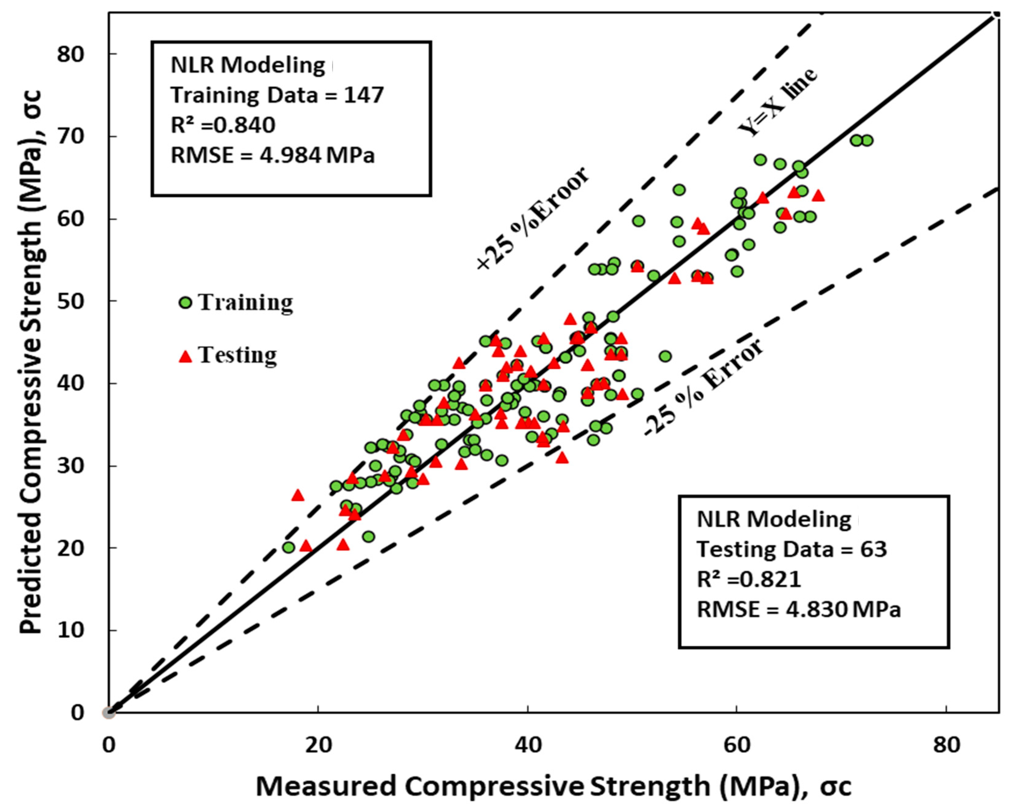
6.2. Nonlinear Regression Model (NLR)

The development of models is essential in predicting the behavior of a system, and nonlinear regression models are often utilized when linear regression models cannot capture the complexity of the system. In this context, a nonlinear regression model (Equation (2)) was developed to predict the compressive strength of concrete using GGBFS while considering factors such as T, w/b, GGBFS/b, w, FA, CA, and SP. This model was used to overcome the limitations of linear regression models, which are unsuitable when the variables are not linearly related. The nonlinear regression model is beneficial in predicting the compressive strength of concrete using GGBFS more accurately [21,22].

$$\begin{gathered} \sigma c={{\beta }_1\left(T\right)}^{{\beta }_2}+{{\beta }_3\left(\frac{w}{b}\right)}^{{\beta }_4}+{{\beta }_5\left(\frac{GGBFS}{b}\right)}^{{\beta }_6}+{{\beta }_7\left(FA\right)}^{{\beta }_8}+{{\beta }_9\left(CA\right)}^{{\beta }_{10}} \\ +{{\beta }_{11}\left(SP\right)}^{{\beta }_{12}}+{\beta }_{13} \end{gathered}$$

(2)

where $\beta$₁–$\beta$₁₃ are model parameters.

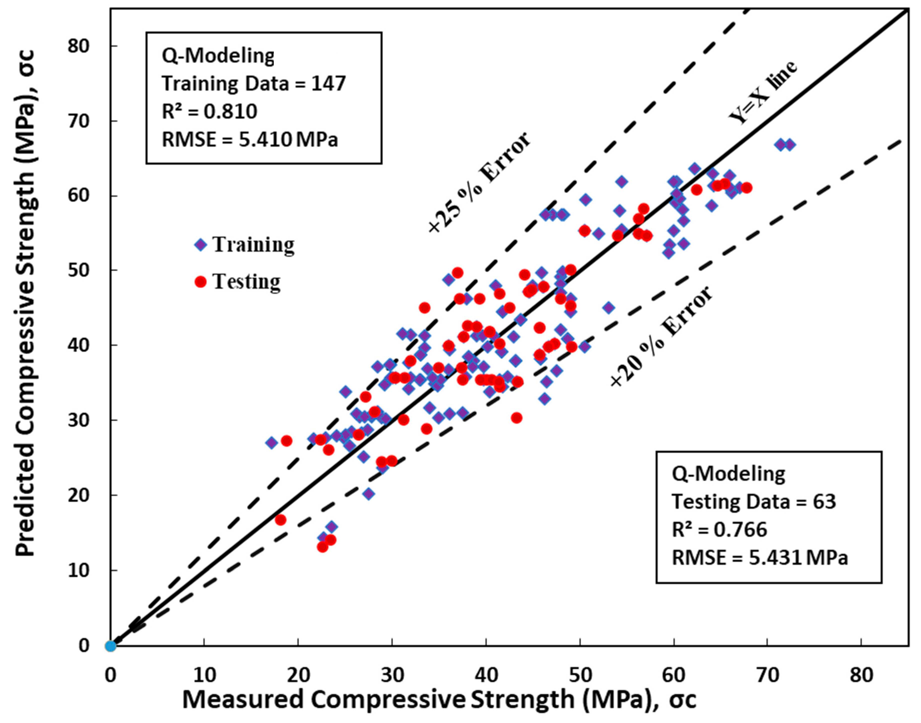
6.3. Quadratic Regression Model (Q)

The quadratic regression model presented in this study represents each parameter through a combination of constant, linear, and squared terms. This formulation enables a more comprehensive and accurate representation of the relationship between the variables being considered. The specific details of the quadratic regression model can be found in Equation (3), which clearly illustrates the model structure and the specific terms used to express each parameter. By utilizing this model, a greater understanding of the underlying factors impacting the compressive strength of the cement paste being investigated was achieved in this study.

$$\begin{array}{ll}\mathsf{\sigma }\mathrm{c}={\beta }_1\left(T\right)+{\beta }_2& \left(\frac{w}{b}\right)+{\beta }_3\left(\frac{GGBFS}{b}\right)+{\beta }_4\left(FA\right)+{\beta }_5\left(CA\right)+{\beta }_6\left(SP\right)+{\beta }_7{\left(T\right)}^2\\ & +{\beta }_8{\left(\frac{w}{b}\right)}^2+{\beta }_9{\left(\frac{GGBFS}{b}\right)}^2+{\beta }_{10}{\left(FA\right)}^2+{\beta }_{11}{\left(CA\right)}^2+{\beta }_{12}{\left(SP\right)}^2\\ & +{\beta }_{13}\end{array}$$

(3)

where $\beta$₁–$\beta$₁₃ are model parameters.

6.4. Full Quadratic Regression Model (FQ)

This study explored the effectiveness of utilizing a full quadratic regression model to predict the compressive strength of cement paste, considering both chemical and mineral compositions. The results of this investigation proved to be quite promising. The full quadratic regression model was evaluated to assess the model’s accuracy in predicting the compressive strength of concrete incorporating GGBFS (ground granulated blast furnace slag). The model consists of squared, linear, interaction (product), and constant terms, all of which are used to express each parameter. The complete formulation of the model is provided in Equation (4).

$$\begin{array}{ll}\mathsf{\sigma }\mathrm{c}={\beta }_1\left(T\right)+{\beta }_2& \left(\frac{w}{b}\right)+{\beta }_3\left(\frac{GGBFS}{b}\right)+{\beta }_4\left(FA\right)+{\beta }_5\left(CA\right)+{\beta }_6\left(SP\right)+{\beta }_7\left(T\right)\left(\frac{w}{b}\right)\\ & +{\beta }_8\left(T\right)\left(\frac{GGBFS}{b}\right){+\beta }_9\left(T\right)\left(FA\right)\\ & +{\beta }_{10}\left(T\right)\left(CA\right){+\beta }_{11}\left(T\right)\left(SP\right){+\beta }_{12}\left(\frac{w}{b}\right)\left(\frac{GGBFS}{b}\right){+\beta }_{13}\left(\frac{w}{b}\right)\left(FA\right){+\beta }_{14}\left(\frac{w}{b}\right)\left(CA\right)\\ & +{\beta }_{15}\left(\frac{w}{b}\right)\left(SP\right){+\beta }_{16}\left(\frac{GGBFS}{b}\right)\left(FA\right){+\beta }_{17}\left(\frac{GGBFS}{b}\right)\left(CA\right)\\ & {+\beta }_{18}\left(\frac{GGBFS}{b}\right)\left(SP\right){+\beta }_{19}\left(FA\right)\left(CA\right){+\beta }_{20}\left(FA\right)\left(SP\right){+\beta }_{21}\left(CA\right)\left(SP\right){+\beta }_{22}{\left(T\right)}^2\\ & {+\beta }_{23}{\left(\frac{w}{b}\right)}^2{+\beta }_{24}{\left(\frac{GGBFS}{b}\right)}^2{+\beta }_{25}{\left(FA\right)}^2{+\beta }_{26}{\left(CA\right)}^2{+\beta }_{27}{\left(SP\right)}^2{+\beta }_{28}\end{array}$$

(4)

where $\beta$₁–$\beta$₈ are model parameters.

6.5. Artificial Neural Network (ANN)

The term artificial neural network (ANN) is derived from biological neural networks that form the structure of a human brain. Like the human brain, which has neurons connected, artificial neural networks also contain interconnected neurons in various layers called nodes [20,21]. These nodes help process data to make predictions or classifications based on the input data. The ANN comprises three layer types: input, output, and hidden layers. The input layer receives the data for analysis, and the output layer produces a result based on the input data and the patterns learned by the network [22]. Computational ANN engines can have unlimited hidden layers, enabling complex data processing [22,23]. To optimize the performance of an ANN, researchers conduct trial iterations to determine the optimal number of hidden layers [23]. In this study, two hidden layers composed of neural networks were chosen for the mode. Statistical parameters such as RMSE, MAE, and R² were used to evaluate the model’s performance, and

Table 2. Statistical measures for assessing the performance of the models.

Datasets	Models	R2	RMSE (MPa)	MAE (MPa)	OBJ (MPa)	Scatter Index
Training	LR	0.834	5.056	4.196	5.251	0.119
	NLR	0.774	4.984	4.052	5.081	0.118
	Quadratic	0.810	5.410	4.498	5.589	0.128
	Full Quadratic	0.810	5.405	4.468	5.576	0.127
	ANN	0.951	4.674	3.786	4.173	0.110
Testing	LR	0.772	5.362	4.480	1.688	0.132
	NLR	0.821	4.830	4.011	1.470	0.118
	Quadratic	0.766	5.431	4.547	1.717	0.134
	Full Quadratic	0.765	6.156	5.437	1.130	0.134
	ANN	0.945	4.080	3.192	1.130	0.100

displays the analysis results. A lower RMSE and MAE, as well as a higher R² value, signify good model performance.

7. Assessment Criteria for Model

The efficiency and quality of the proposed models have been thoroughly examined in this study by utilizing various key parameters. These parameters include the coefficient of determination (R²), root mean square error (RMSE), mean absolute error (MAE), scatter index (SI), and objective functions (OBJs), which are essential tools for determining the overall suitability and performance of the proposed models. Specifically, R² measures the correlation between the predicted and actual values, with values closer to 1 indicating a stronger correlation [24]. RMSE and MAE, on the other hand, measure the accuracy of the predictions, with lower values indicating higher accuracy [25]. In addition, the SI is utilized to assess the degree of scatter or variability in the data, with lower values indicating less scatter. Finally, the OBJ refers to the function being optimized by the model.

$$R^2={\left(\frac{\sum _i(xi-\overline{x})\times (yi-\overline{y})}{\sqrt{\sum _i{(xi-\overline{x})}^2}\times \sqrt{\sum _i{(yi-\overline{y})}^2}}\right)}^2$$

(5)

$$RMSE=\sqrt{\frac{\sum _{i=1}^n{(yi-xi)}^2}{n}}$$

(6)

$$MAE=\frac{\sum _{i=1}^n{\left(yi-xi\right)}^2}{n}$$

(7)

$$SI=\frac{RMSE}{yi}$$

(8)

$$OBJ=\left(\frac{n_{tr}}{n_{all}}\times \frac{{{RMSE}_{tr}+MAE}_{tr}}{R_{tr}^2+1}\right)+\left(\frac{n_{tst}}{n_{all}}\times \frac{{{RMSE}_{tst}+MAE}_{tst}}{R_{tst}^2+1}\right)$$

(9)

In the above equations, the following variables are used: $yi$, which represents the experimental value; xi, which represents the predicted value according to the proposed model; $\overline{y}$, which represents the average value of all experimental values; $\overline{x}$, which represents the average of all predicted values; and n, which represents the total number of data points.

The scatter index (SI) is a measure used in optimization algorithms to evaluate the diversity or dispersion of a set of solutions in a multi-objective optimization problem. In multi-objective optimization, the goal is to find solutions representing a trade-off between multiple conflicting objectives. The scatter index quantifies the distribution of solutions across the objective space. A lower scatter index indicates a more uniform distribution of solutions, implying a diverse set that covers different regions of the objective space. On the other hand, a higher scatter index suggests that the solutions are concentrated in specific regions of the objective space, potentially indicating a lack of diversity. In optimization, an objective function (OBJ) is a mathematical representation of the goal or objective to be optimized. In multi-objective optimization, multiple objective functions must be simultaneously optimized. Each objective function represents a different aspect or criterion to be considered. In summary, the scatter index measures the dispersion of solutions in the objective space, indicating the diversity of the solutions. Objective functions represent the different criteria or goals for optimization in a multi-objective optimization problem.

8. Results and Discussions

8.1. Linear Regression Model (LR)

Figure 4 presents a graphical representation of the relationship between concrete’s predicted and actual compressive strength using GGBFS/b enhanced with a superplasticizer. The model employed in this study expresses each input function linearly, as shown in Equation (10):

$$\begin{gathered} \begin{array}{ll}\mathsf{\sigma }\mathrm{c}=0.05\left(T\right)-& 114.5\left(\frac{w}{b}\right)-3.8\left(\frac{GGBFS}{b}\right)-0.02\left(FA\right)+0.12\left(CA\right)-364\left(SP\right) \\ \\ & -3.53\end{array} \end{gathered}$$

(10)

LR modeling shows that SP and w/b have the most significant impact on the compressive strength of concrete, while GGBFS/b also has an apparent effect among all other model parameters. This result suggests that using GGBFS/b in concrete mix design can substantially enhance its strength. The statistical analysis presented in

Table 3. Assessing Model Performance in Predicting Compressive Strength Across Various Ranges.

Models	Compressive Strength Ranges (MPa)	No. of Data	R2	RMSE (MPa)	MAE (MPa)	Scatter Index	Model Performance
LR	15–25	13	0.931	5.198	4.699	0.237	Excellent
	25–40	83	0.730	5.254	4.312	0.160	good
	40–60	91	0.522	5.129	4.218	0.109	poor
	60–75	23	0.956	4.813	4.182	0.074	Excellent
NLR	15–25	13	0.962	3.998	3.406	0.182	Excellent
	25–40	83	0.813	4.494	3.799	0.137	Very good
	40–60	91	0.353	5.734	4.706	0.122	Poor
	60–75	23	0.979	3.250	2.632	0.050	Excellent
Pure Quadratic	15–25	13	0.883	6.742	6.142	0.307	Very good
	25–40	83	0.742	5.137	4.254	0.156	good
	40–60	91	0.410	5.708	4.715	0.121	poor
	60–75	23	0.965	4.244	3.725	0.066	Excellent
Full Quadratic	15–25	13	0.884	6.721	6.104	0.305	Very good
	25–40	83	0.750	5.082	4.167	0.155	good
	40–60	91	0.400	5.751	4.746	0.122	poor
	60–75	23	0.964	4.258	3.740	0.065	Excellent
ANN	15–25	13	0.956	4.200	3.144	0.191	Excellent
	25–40	83	0.680	5.667	4.875	0.173	poor
	40–60	91	0.760	3.635	2.888	0.077	good
	60–75	23	0.987	2.662	2.147	0.041	Excellent

confirms the accuracy of the model, as evidenced by the low RMSE values of 5.06 MPa and 5.36 MPa for training and testing datasets, respectively. Moreover, the coefficient of determination R² values of 0.83 and 0.77 for training and testing, respectively, indicate that the model can predict the compressive strength of concrete with a high degree of accuracy.

Overall, these results demonstrate that using GGBFS/b in concrete mix design, enhanced with a superplasticizer, can significantly improve the strength of concrete and that the developed model performs exceptionally well in predicting the compressive strength of concrete.

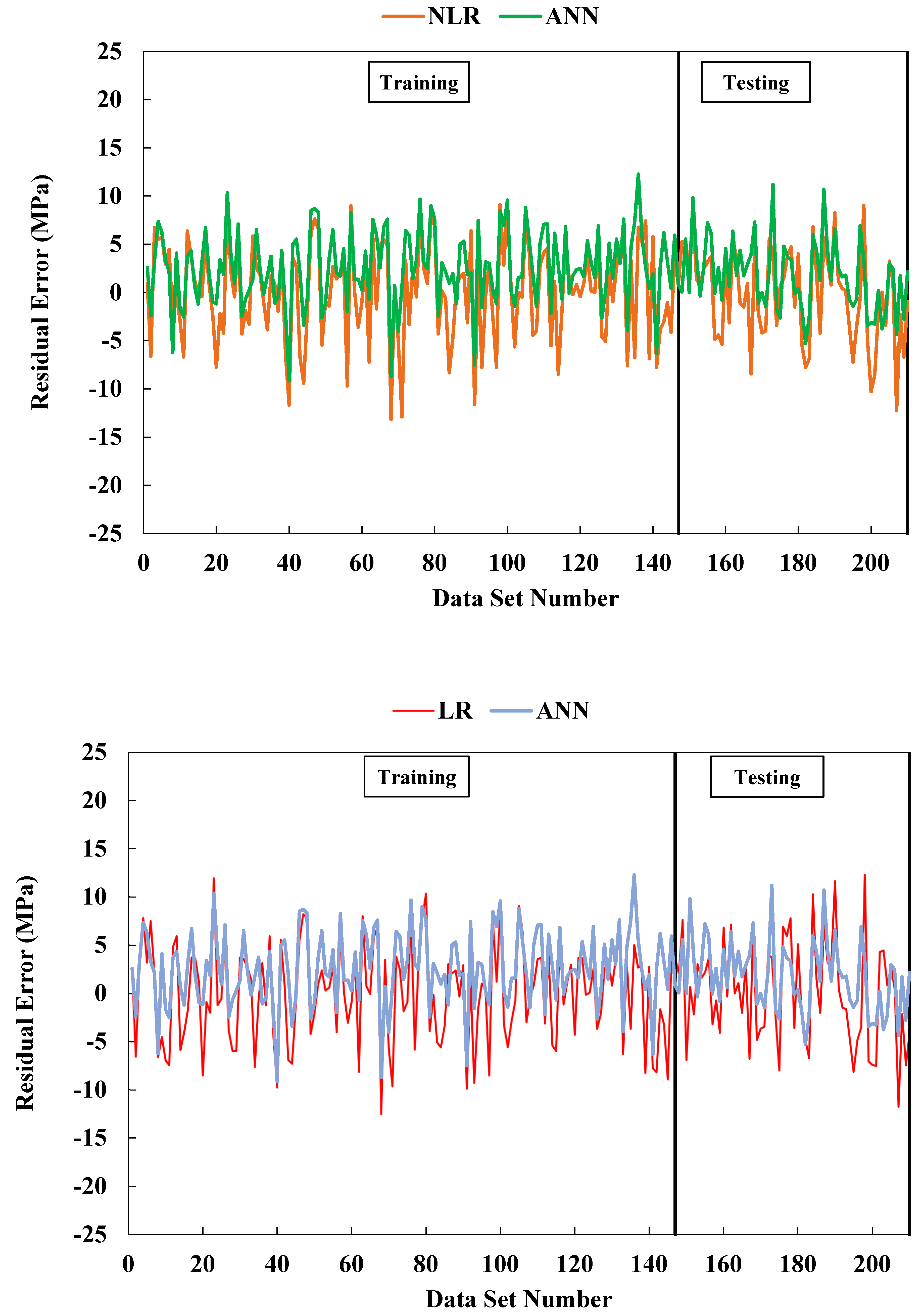
8.2. Nonlinear Regression Model (NLR)

The exposed model was evaluated to predict the compressive strength of GGBFS/b concrete and superplasticizer using a nonlinear model, as shown in Equation (11).

$$\begin{gathered} \sigma c={-123.6\left(T\right)}^{-1.7}+{1590.1\left(\frac{w}{b}\right)}^{-0.03}+{0.06\left(\frac{GGBFS}{b}\right)}^{-0.2}+{182.3\left(FA\right)}^{-0.05} \\ +{0.01\left(CA\right)}^{1.26}{-0.01\left(SP\right)}^{6.4}-1784.1 \end{gathered}$$

(11)

The performance of this model was evaluated based on the root mean square error (RMSE) and coefficient of determination. The RMSE values for the training and test data sets were 4.98 MPa and 4.83 MPa, respectively. The coefficient of determination of the data sets was 0.77 and 0.82, respectively, as displayed in Table 3 and Figure 5. Based on these results, it can be concluded that the nonlinear model can accurately predict the compressive strength of concretes using GGBFS/b and the superplasticizer, as indicated by the R² values high and low RMSE values.

8.3. Quadratic Regression Model (Q)

The quadratic model developed in this study involves each parameter expressed in constant, linear, and squared terms. The resulting model is depicted in Equation (12).

$$\begin{gathered} \mathsf{\sigma }\mathrm{c}=0.02\left(T\right)-110\left(\frac{w}{b}\right)-+0.1\left(CA\right)-2.3\left(SP\right)+0.3{\left(\frac{w}{b}\right)}^2 \\ +6.3{\left(\frac{GGBFS}{b}\right)}^2{-6.4\left(FA\right)}^2+3.3{\left(CA\right)}^2+0.01{\left(SP\right)}^2+0.5 \end{gathered}$$

(12)

The performance of this model was evaluated using the root mean square error (RMSE) and coefficient of determination (R²). The RMSE values for the training and testing datasets were 5.41 MPa and 5.43 MPa, respectively. Furthermore, the R² values for the training and testing datasets of the quadratic model were 0.81 and 0.77, respectively, as presented in Table 3. The relationship between the predicted compressive strength and measured compressive strength for the quadratic model is illustrated in Figure 6. These results demonstrate that the quadratic model accurately predicts the compressive strength of concrete, as evidenced by the high R² values and relatively low RMSE values.

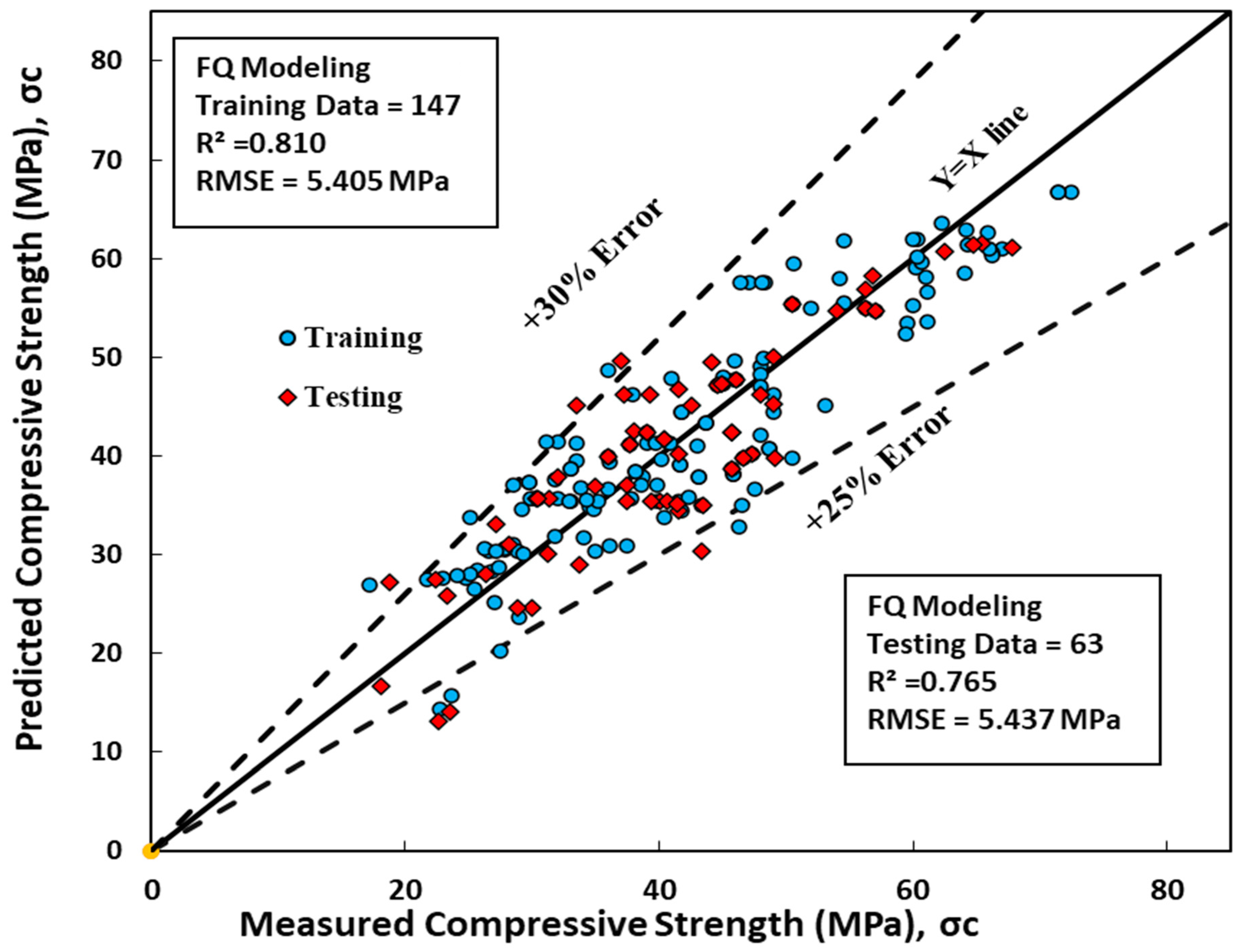
8.4. Full Quadratic Regression Model (FQ)

The full quadratic model was developed and evaluated to predict the compressive strength of concrete with GGBFS/b enhanced with a superplasticizer. This model expressed each parameter in constant, linear, interaction (product), and squared terms. The resulting model is presented in Equation (13):

$$\begin{gathered} \begin{array}{ll}\mathsf{\sigma }\mathrm{c}=110.1\left(\frac{w}{b}\right)& -0.03\left(\frac{GGBFS}{b}\right)-0.01\left(FA\right)+0.1\left(CA\right)-2.3\left(SP\right)\\ & \\ +0.3\left(T\right)\left(\frac{GGBFS}{b}\right)-6.5\left(T\right)\left(CA\right)+0.1\left(\frac{w}{b}\right)\left(\frac{GGBFS}{b}\right)\\ & +0.5\left(\frac{w}{b}\right)\left(FA\right)-0.5\left(\frac{w}{b}\right)\left(CA\right)+0.4\left(\frac{w}{b}\right)\left(SP\right)\\ & +0.3\left(\frac{GGBFS}{b}\right)\left(FA\right)-0.7\left(\frac{GGBFS}{b}\right)\left(CA\right)\\ & -48.5\left(\frac{GGBFS}{b}\right)\left(SP\right)-0.04{\left(T\right)}^2-0.03{\left(\frac{GGBFS}{b}\right)}^2\\ & +0.06{\left(SP\right)}^2\end{array} \end{gathered}$$

(13)

The performance of the full quadratic model was assessed using the root mean square error (RMSE) and coefficient of determination (R²). The RMSE values for the training and testing datasets were 5.41 MPa and 6.156 MPa, respectively, as shown in Table 3. Moreover, the R² values for the training and testing datasets of the full quadratic model were 0.81 and 0.77, respectively, as depicted in Figure 7. The results indicate that the full quadratic model parameters are comparable to those of the previous models (linear, nonlinear, and quadratic models) in predicting the compressive strength of concrete with GGBFS/b enhanced with a superplasticizer, as evidenced by the relatively high R² values.

8.5. Artificial Neural Network (ANN)

Selecting appropriate input variables is crucial in system modeling since the selected variables should contain all the relevant information to achieve the desired output values. In this study, six distinct parameters were considered to predict the compressive strength of normal concrete, including temperature, w/b ratio, and GGBFS/b, fine aggregate, coarse aggregate, and superplasticizer. Two hidden layers, including two neural networks, were used with a learning rate of 0.2, momentum of 0.1, and a training length of 2000. The number of epochs is a hyperparameter that determines the learning algorithm processes of the training dataset. A higher number of epochs lead to a higher R² and lower RMSE and MAE values, as the model minimizes error (Figure 8). The anticipated compressive strength vs. the actual value is depicted in Figure 9, showcasing the fundamental idea of data generated using an ANN model. According to statistical variables, the ANN model predicts the compressive strength of conventional concrete more accurately than do other models such as LR, NLR, quadratic, and full quadratic models. The training dataset’s R², RMSE, and MAE values are 0.95, 4.67 MPa, and 3.79 MPa, respectively. Moreover, the SI value and objective for the current model are 0.11 and 4.17 MPa, respectively, as shown in Table 3. The testing dataset results show an R² value of 0.95 and RMSE and MAE values of 4.08 MPa and 3.19 MPa, respectively, along with a SI of 0.10 and an objective of 1.1 MPa (Figure 9).

9. Model Comparison

The study aimed to assess the performance of different models in predicting the compressive strength of recycled aggregate concrete containing GGBFS/b. Four statistical measures, namely RMSE, R2, OBJ, MAE, and SI, were employed to evaluate the effectiveness of these models. Based on the results, the artificial neural network (ANN) model outperformed the other models significantly regarding the R2, RMSE, and MAE values, as demonstrated in Figure 10. This indicates that the ANN model predicted the concrete’s compressive strength more accurately than the alternative models did. All models demonstrated SI values within the excellent performance range of 0.10 to 0.13, implying their overall effectiveness, as depicted in Table 3. However, it is worth noting that the ANN model exhibited smaller SI values than the other models did, as illustrated in Figure 11. This suggests that the predictions made by the ANN model were more consistent and closer to the actual values.

Furthermore, this study analyzed the scatter index value for each model. The ANN model exhibited a smaller scatter index value compared to that of the other models, with a difference of 7.50% from the linear regression model, 6.80% from the nonlinear regression model, 14.06% from the quadratic regression model, and 13.39% from the full quadratic regression model for the training dataset. This finding indicates that the ANN model had a lower level of dispersion in its predictions, making it more reliable. Additionally, the OBJ function values for the ANN model were significantly lower than those of the other models, both for the training and testing datasets. Specifically, the ANN model achieved OBJ values that were 20.5% less than those of the linear regression model, 15.53% less than those of the nonlinear regression model, 25.33% less than those of the quadratic regression model, and 25.16% less than those of the full quadratic regression model for the training dataset, as presented in Figure 12. This suggests that the ANN model better fits the data and minimizes the objective function more effectively. To visually illustrate the performance of the models, we plotted the residual errors for the training and testing datasets in Figure 13. The plot revealed that the ANN model’s predicted and measured compressive strengths were more consistent than those of the other models. This observation suggests that the ANN model was more effective at predicting the compressive strength of concrete containing GGBFS, emphasizing its superior accuracy in calculating the compressive strength. This higher accuracy can lead to more reliable and efficient construction practices.

Furthermore, the ANN model exhibited a percentage error between +35% and −20%, indicating its high accuracy in predicting the concrete’s compressive strength. Using GGBFS as a substitute for Portland cement in concrete resulted in varying compressive strength ranges, as observed in previous studies. Various models were tested to predict the high compressive strength of GGBFS concrete, and the ANN model consistently outperformed the others. Remarkably, the ANN model achieved an R² value of 0.99 and the lowest RMSE value of 2.66 MPa within the compressive strength range of 60–75 MPa, according to Table 3. However, the 25–60 MPa range was identified as the most reliable range for the models, given its larger dataset of 174 data points, as demonstrated in Table 3. Within this range, the models were further divided into two sub-ranges due to the weaknesses observed in the 40–60 MPa range, with better model performance recorded in the 25–40 MPa range.

10. Sensitivity Analysis

The degree to which input factors affect the output parameter was determined using the sensitivity analysis approach in this study. To conduct this analysis, the quadratic model was employed to predict the compressive strength of concrete that contained GGBFS as a replacement for Portland cement. The sensitivity analysis of the quadratic model concerning the input parameters produced several noteworthy findings. The water-to-binder ratio was observed to have the most significant role in determining the compressive strength of concrete. Specifically, when this input factor was removed, the R² value decreased to 0.62, and the RMSE was at its highest at 7.68 MPa, as indicated in

Table 4. Sensitivity analysis applying Q-Model to the training dataset.

No.	Combination	Removed Parameter	R2	RMSE (MPa)	MAE (MPa)	Ranking
All	T, w/b, GGBFS/b, FA, CA, and SP	None	0.810	5.410	4.498	-
1	w/b, GGBFS/b, FA, CA, and SP	T	0.808	5.435	4.580	3
2	T, GGBFS/b, FA, CA, and SP	w/b	0.620	7.679	5.955	1
3	T, w/b, FA, CA, and SP	GGBFS/b	0.810	5.412	4.500	6
4	T, w/b, GGBFS/b, CA, and SP	FA	0.764	6.022	5.087	2
5	T, w/b, GGBFS/b, FA, and SP	CA	0.820	5.263	4.092	4
6	T, w/b, GGBFS/b, FA, and CA	SP	0.810	5.414	4.502	5

.

Regarding GGBFS, it was found to have a medium effect and was ranked fourth out of the six input parameters used in this study. This implies that GGBFS had a normal effect, much like the other input factors. The R² values for the other input parameters, excluding the water-to-binder ratio, were similar to those for Ground granulated blast-furnace slag (GGBFS) content, indicating that it had a comparable effect. Overall, the sensitivity analysis results using the quadratic model provide insights into the relative impact of input factors on the compressive strength of concrete with GGBFS as a cement substitute. These findings can be utilized to optimize the design of concrete mixtures containing GGBFS, leading to more sustainable and desirable construction materials.

11. Conclusions

This study focused on the accuracy of different models in predicting the compressive strength of concrete containing GGBFS using data from the literature and the influences of various parameters on the compressive strength. The following conclusions were reported:

• Insignificant relationships were found between the input parameters and compressive strength, indicating the influence of multiple factors on concrete compressive strength.
• The correlation matrix analysis emphasized the need to consider multiple parameters, as no single attribute alone can determine compressive strength.
• Different models, including linear regression, nonlinear regression, quadratic, and full quadratic models were developed to predict compressive strength, considering various parameters and their interactions.
• An artificial neural network (ANN) model captured complex relationships within the dataset.
• Overall, the sensitivity analysis results derived from the quadratic model provide valuable insights into the relative impact of input factors on the compressive strength of concrete when GGBFS is employed as a cement substitute.
• The ANN model was the most reliable model in predicting the compressive strength of concrete containing GGBSF.
• The study contributes to a better understanding of factors influencing the compressive strength of GGBFS-containing concrete and provides insights for optimizing concrete mixtures and cement replacement with GGBFS.
• The developed models offer practical tools for optimizing concrete mixtures, enhancing durability, and promoting sustainable design principles.
• Adopting these approaches can contribute to global efforts in mitigating climate change and achieving a more sustainable future in the construction industry.
• Sensitivity analysis of the results revealed several significant findings concerning the compressive strength of concrete, particularly concerning the quadratic model and its corresponding input parameters. The water-to-binder ratio was identified as the most influential factor in determining the compressive strength, indicating that GGBFS exhibited behavior similar to that of other input factors.
• Based on the model outcomes, the w/b has the greatest impact on the change in the compressive strength of concrete than did the other model parameters.

References

1. Flatt, R.J.; Roussel, N.; Cheeseman, C.R. Concrete: An eco material that needs to be improved. J. Eur. Ceram. Soc. 2012, 32, 2787–2798. [Google Scholar] [CrossRef]
2. Badogiannis, E.; Papadakis, V.; Chaniotakis, E.; Tsivilis, S. Exploitation of poor Greek kaolins: Strength development of metakaolin concrete and evaluation by means of k-value. Cem. Concr. Res. 2004, 34, 1035–1041. [Google Scholar] [CrossRef]
3. Roy, D.; Arjunan, P.; Silsbee, M. Effect of silica fume, metakaolin, and low-calcium fly ash on chemical resistance of concrete. Cem. Concr. Res. 2001, 31, 1809–1813. [Google Scholar] [CrossRef]
4. Ferraris, C.F.; Obla, K.H.; Hill, R. The influence of mineral admixtures on the rheology of cement paste and concrete. Cem. Concr. Res. 2001, 31, 245–255. [Google Scholar] [CrossRef]
5. Chan, W.; Wu, C. Durability of concrete with high cement replacement. Cem. Concr. Res. 2000, 30, 865–879. [Google Scholar] [CrossRef]
6. Behnood, A.; Golafshani, E.M. Predicting the compressive strength of silica fume concrete using hybrid artificial neural network with multi-objective grey wolves. J. Clean. Prod. 2018, 202, 54–64. [Google Scholar] [CrossRef]
7. Kumar, R.; Samanta, A.K.; Roy, D.S. Characterization and development of eco-friendly concrete using industrial waste—A Review. J. Urban Environ. Eng. 2014, 8, 98–108. [Google Scholar] [CrossRef] [Green Version]
8. Oner, A.; Akyuz, S. An experimental study on optimum usage of GGBS for the compressive strength of concrete. Cem. Concr. Compos. 2007, 29, 505–514. [Google Scholar] [CrossRef]
9. Chidiac, S.; Panesar, D. Evolution of mechanical properties of concrete containing ground granulated blast furnace slag and effects on the scaling resistance test at 28 days. Cem. Concr. Compos. 2008, 30, 63–71. [Google Scholar] [CrossRef]
10. Cheng, A.; Huang, R.; Wu, J.-K.; Chen, C.-H. Influence of GGBS on durability and corrosion behavior of reinforced concrete. Mater. Chem. Phys. 2005, 93, 404–411. [Google Scholar] [CrossRef]
11. Song, H.-W.; Saraswathy, V. Studies on the corrosion resistance of reinforced steel in concrete with ground granulated blast-furnace slag—An overview. J. Hazard. Mater. 2006, 138, 226–233. [Google Scholar] [CrossRef]
12. Pal, S.; Mukherjee, A.; Pathak, S. Investigation of hydraulic activity of ground granulated blast furnace slag in concrete. Cem. Concr. Res. 2003, 33, 1481–1486. [Google Scholar] [CrossRef]
13. Saafan, M.A.; Etman, Z.A.; El Lakany, D.M. Microstructure and Durability of Ground Granulated Blast Furnace Slag Cement Mortars. Iran. J. Sci. Technol. Trans. Civ. Eng. 2021, 45, 1457–1465. [Google Scholar] [CrossRef]
14. Douglas, E.; Zerbino, R. Characterization of granulated and pelletized blast furnace slag. Cem. Concr. Res. 1986, 16, 662–670. [Google Scholar] [CrossRef]
15. Xu, H.; Gong, W.; Syltebo, L.; Izzo, K.; Lutze, W.; Pegg, I.L. Effect of blast furnace slag grades on fly ash based geopolymer waste forms. Fuel 2014, 133, 332–340. [Google Scholar] [CrossRef]
16. Elibol, C.; Sengul, O. Effects of activator properties and ferrochrome slag aggregates on the properties of alkali-activated blast furnace slag mortars. Arab. J. Sci. Eng. 2015, 41, 1561–1571. [Google Scholar] [CrossRef]
17. Norrarat, P.; Tangchirapat, W.; Songpiriyakij, S.; Jaturapitakkul, C. Evaluation of Strengths from Cement Hydration and Slag Reaction of Mortars Containing High Volume of Ground River Sand and GGBF Slag. Adv. Civ. Eng. 2019, 2019, 1–12. [Google Scholar] [CrossRef] [Green Version]
18. Sarwar, W.; Ghafor, K.; Mohammed, A. Regression analysis and Vipulanandan model to quantify the effect of polymers on the plastic and hardened properties with the tensile bonding strength of the cement mortar. Results Mater. 2019, 1, 100011. [Google Scholar] [CrossRef]
19. Sarwar, W.; Ghafor, K.; Mohammed, A. Modeling the rheological properties with shear stress limit and compressive strength of ordinary Portland cement modified with polymers. J. Build. Pathol. Rehabil. 2019, 4, 25. [Google Scholar] [CrossRef]
20. Ghafor, K.; Qadir, S.; Mahmood, W.; Mohammed, A. Statistical variations and new correlation models to predict the mechanical behaviour of the cement mortar modified with silica fume. Géoméch. Geoengin. 2020, 17, 118–130. [Google Scholar] [CrossRef]
21. Ahmed, H.U.; Mohammed, A.A.; Mohammed, A. Soft computing models to predict the compressive strength of GGBS/FA-geopolymer concrete. PLoS ONE 2022, 17, e0265846. [Google Scholar] [CrossRef] [PubMed]
22. Ahmed, H.U.; Abdalla, A.A.; Mohammed, A.S.; Mohammed, A.A.; Mosavi, A. Statistical Methods for Modeling the Compressive Strength of Geopolymer Mortar. Materials 2022, 15, 1868. [Google Scholar] [CrossRef] [PubMed]
23. Vujičić, T.; Matijevi, T.; Ljucović, J.; Balota, A.; Ševarac, Z. Comparative analysis of methods for determining number of hidden neurons in artificial neural network. In Proceedings of the Central European Conference on Information and Intelligent Systems, Varazdin, Croatia, 21–23 September 2016; Volume 219. [Google Scholar]
24. Ozer, D.J. Correlation and the coefficient of determination. Psychol. Bull. 1985, 97, 307. [Google Scholar] [CrossRef]
25. Wang, W.; Lu, Y. Analysis of the Mean Absolute Error (MAE) and the Root Mean Square Error (RMSE) in Assessing Rounding Model. IOP Conf. Ser. Mater. Sci. Eng. 2018, 324, 012049. [Google Scholar] [CrossRef]
26. Lee, K.; Lee, H.; Lee, S.; Kim, G. Autogenous shrinkage of concrete containing granulated blast-furnace slag. Cem. Concr. Res. 2006, 36, 1279–1285. [Google Scholar] [CrossRef]
27. Kwang-Myong, L.; Ki-Heon, K.; Hoi-Keun, L.; Seung-Hoon, L.; Gyu-Yong, K. Characteristics of autogenous shrinkage for concrete containing blast-furnace slag. J. Korea Concr. Inst. 2004, 16, 621–626. [Google Scholar]
28. Wainwright, P.; Rey, N. The influence of ground granulated blastfurnace slag (GGBS) additions and time delay on the bleeding of concrete. Cem. Concr. Compos. 2000, 22, 253–257. [Google Scholar] [CrossRef]
29. Li, Q.T.; Li, Z.G.; Yuan, G.L. Effects of elevated temperatures on properties of concrete containing ground granulated blast furnace slag as cementitious material. Constr. Build. Mater. 2012, 35, 687–692. [Google Scholar] [CrossRef]
30. Han, I.-J.; Yuan, T.-F.; Lee, J.-Y.; Yoon, Y.-S.; Kim, J.-H. Learned prediction of compressive strength of GGBFS concrete using hybrid artificial neural network models. Materials 2019, 12, 3708. [Google Scholar] [CrossRef] [Green Version]
Figure 1. The flowchart diagram process followed in this study.
Sustainability 15 11907 g001
Figure 2. Marginal plot for the compressive strength of GGBFS concrete versus (a) temperature, (b) water to binder ratio, (c) Ground granulated blast-furnace slag to binder ratio, and water, (d) fine aggregate, (e) coarse aggregate, (f) superplasticizer content.
Sustainability 15 11907 g002
Figure 3. Correlation matrix plot for input and output variables.
Sustainability 15 11907 g003
Figure 4. Comparison between measured and predicted compressive strength using linear regression model (lr) for training and testing data sets.
Sustainability 15 11907 g004
Figure 5. Comparison between measured and predicted compressive strength using nonlinear regression model (NLR) for training and testing datasets.
Sustainability 15 11907 g005
Figure 6. Comparison between measured and predicted compressive strength using quadratic regression model (Q) for training and testing datasets.
Sustainability 15 11907 g006
Figure 7. Comparison between measured and predicted compressive strength using full-quadratic regression model (FQ) for training and testing datasets.
Sustainability 15 11907 g007
Figure 8. The standard structure of a neural network model.
Sustainability 15 11907 g008
Figure 9. Comparison between measured and predicted compressive strength using artificial neural network model (ANN) for training and testing datasets.
Sustainability 15 11907 g009
Figure 10. Model comparison between linear regression (LR), nonlinear regression (NLR), quadratic (Q), full quadratic (FQ), and artificial neural network (ANN) for (a) training and (b) testing data sets.
Sustainability 15 11907 g010
Figure 11. Comparison of the SI performance parameter of different developed models for (a) training and (b) testing data sets.
Sustainability 15 11907 g011
Figure 12. The OBJ function values in (MPa) for all developed models for compressive strength for training and testing data sets.
Sustainability 15 11907 g012
Figure 13. Residual error of compressive strength using training and testing datasets.
Sustainability 15 11907 g013aSustainability 15 11907 g013b