Carbon Storage Estimation of Quercus aquifolioides Based on GEDI Spaceborne LiDAR Data and Landsat 9 Images in Shangri-La

Abstract

The assessment of forest carbon storage plays a crucial role in forest management and ecosystem exploration, enabling the evaluation of forest quality, resources, carbon cycle and management. The Global Ecosystem Dynamics Investigation (GEDI) satellite provides a means to accurately measure these various forest vertical structure parameters by penetrating the forest canopy. However, the distribution of the footprint along the orbit track is heterogeneous and discontinuous, preventing the acquisition of spatially distributed carbon storage formation at the county level. Consequently, this study integrated GEDI and Landsat 9 data to estimate Quercus aquifolioides carbon storage in Shangri-La. By applying the Kriging interpolation to previously pretreated footprints, surface information from the GEDI L2B footprints was obtained. At the same time, Landsat 9 vegetation indices and band reflectance were extracted to analyze the correlation with the carbon storage of Quercus aquifolioides samples. Then, three methods (support vector machine, bagging, and random forest) were used to create a carbon storage estimation model for Shangri-La. The research results showed that (1) among the models for the selection of GEDI footprint parameters based on semi-variance, the optimal model of the digital_elevation_model was the spherical model, while the best model of percentage tree cover from the MODIS data (modis_treecover) and the foliage height diversity index (fhd_normal) was the exponential model. (2) Analyzing the thirty-three extracted independent variable factors correlated with the carbon storage of Quercus aquifolioides showed that the top five variables with the highest correlation were digital_elevation_model, modis_treecover, fhd_normal, DEM, and band 1 (B1). (3) After variable selection, the R² = 0.82 and RMSE = 11.92 t/hm² values of the Quercus aquifolioides carbon storage estimation model established via random forest were obtained, and its evaluation precision was superior to that of the support vector machine method and bagging regression. The carbon storage of Quercus aquifolioides was primarily in the range of 8.22~94.63 t/hm², and the mean value was 42.44 t/hm², while the total carbon storage was about 5,374,137.62 t. The findings from this paper illustrated the feasibility of obtaining carbon storage data on a county scale by combining GEDI LiDAR data with Landsat 9 optical data. The results also suggested a new perspective for combining GEDI L2B data with other remote sensing images to estimate other forest structure parameters.

1. Introduction

The global forest area, although occupying only 1/3 of the terrestrial area, plays a crucial role in carbon storage within terrestrial ecosystems. Forest vegetation alone accounts for half of the terrestrial carbon pool [1] and stores 60% of the carbon ecosystem. Thus, forest land acts as the largest “carbon storage pool” and the most efficient “carbon absorber” [2]. Moreover, forests possess a powerful carbon-sinking ability that is vital for balancing and regulating atmospheric carbon dioxide [3]. Given the complexity and enormity of the global ecosystem mechanisms, even minor changes can have a substantial impact [4].

In forest ecosystems, biomass is multiplied by carbon content to obtain the plant carbon storage, while the distribution of carbon storage in forest ecosystems is basically consistent with the pattern of its biomass [5]. The precise assessments of forest biomass and its variation have provided scientific evidence for carbon storage estimation, which is essential for exploring the carbon cycle of terrestrial ecosystems and moderating the ecosystem processes [6]. Due to the rapid advancement of quantitative remote sensing technology, the findings of remote sensing-based carbon storage estimations are becoming extremely consistent and dependable. Therefore, remote sensing methods have become a major tool for quantifying forest carbon storage on a larger scale [7]. However, many works have illustrated that methods which use optical remote sensing data alone are limited by the saturation effect of optical sensors [8]. Synthetic aperture radar (SAR) can acquire data around the clock at any time, in any weather, and its ability to penetrate vegetation varies with different wavelengths. Vegetation carbon storage can be retrieved by using its backscatter intensity signal and its derivative characteristics [9]. LiDAR is an active remote sensing technology that uses short wavelength laser pulses to penetrate forest canopies and obtain vertical structure information [10]. The ability of LiDAR to detect the vertical structure of forests has proven to be effective in studying forest carbon storage estimation in various forest environments. At present, even in forests with high aboveground biomass (AGB) levels, saturation is rarely observed when using LiDAR methods [11]. Compared to the optical images and SAR, the use of LiDAR significantly improves the accuracy of estimating forest carbon storage. However, LiDAR currently has shortcomings in terms of spatial and temporal coverage, which limit its application in global forest carbon storage estimation.

The launch of GEDI, a LiDAR system developed to monitor the vertical structure of forests, presents a unique opportunity for improving vertical forest structure mapping [12]. GEDI’s space-based mission is specifically designed to explore vegetation structures and estimate aboveground carbon stocks in temperate and tropical forest and woodlands. To achieve this, GEDI utilizes a 25-meter-diameter footprint of full waveform LiDAR data for estimating vegetation structures between 51.6° north and south [13]. The GEDI data are divided into four levels, each providing different levels of vegetation information. Many studies have utilized Level 2 canopy height and Level 4 footprint biomass products to evaluate the accuracy of GEDI in estimating forest structural parameters. By obtaining accurate structural measurements of canopy relative height (RH) metrics from GEDI L2A products, Iván et al. [14] estimated the AGB of various forest ecosystems at the laser footprint level by applying ALS-derived biomass models. And the AGB values estimated at different footprint levels of various forest types were applied as independent variables, while relative height metrics (rh60, rh70, rh80, rh90, rh95, rh98, and rh99) extracted from GEDI L2A and canopy profile metrics (cover, pgap_thea, pai, and fhd_normal) extracted from L2B were used as explanatory variables to construct GEDI footprint-level biomass estimation models for each forest type. Additionally, large-scale biomass products can be obtained from L4A footprint biomass measurements. Dan et al. [15] evaluated the AGB prediction results extracted from GEDI L4A products and generated AGB maps using ground survey samples. The results demonstrated that the AGB prediction results from the GEDI L4A products performed poorly in different AFS models in west Africa, with an 8.94-fold higher forecasting error compared to the estimation based on GEDI L4A. It should be noted that this product is only available in the Guineo-Congolian region.

However, because GEDI is discretely sampled along the track, its footprint is spatially discontinuous. There existed certain limitations in predicting vegetation structures information solely with GEDI data. It is difficult to directly provide continuous coverage of canopy height or AGB map without using other methods. Consequently, some scholars had combined GEDI data with other remote sensing data such as MODIS, SAR, Sentinel, and SPOT to obtain continuous information, making-up for the lack of GEDI data alone. Yuri et al. [16] proposed a method to generate a wall-to-wall AGBD mapping which depended merely on open access earth observation data. The suitability of this approach for a wide range of geographic areas was examined and compared with the current worldwide AGBD results. For this purpose, GEDI data were integrated with Sentinel-1, Sentinel-2, and altitude data to generate the all-weather AGBD maps for Australia and the United States in 2020. This data integration approach used to produce more accurate and less saturated results in high biomass areas compared to using a single data source. Carlos et al. [17] developed a multi-sensor data fusion method using GEDI, ICESat-2, and NISAR data to produce wall-to-wall AGB maps. This verification demonstrated that fusion framework provided more accurate AGB estimates than using GEDI or ICESat-2 data alone. Liu et al. [18] discovered a strong correlation between the forest canopy heights represented by rh96 in GEDI L2A and airborne forest canopy height. They combined rh96 with spectral information and vegetation indices from optical remote sensing images (Landsat8 OLI, Sentinel-1, and Sentinel-2), and established a forest canopy height inversion model using the random forest algorithm. This allowed them to achieve a forest height mapping at a resolution of 30 m in the Yunnan Province. Camile et al. [19] discovered that the L-band of ALOS-2/PALSAR-2 deeply penetrated the forest canopy and provided more accurate information about the vertical structure of vegetation. Therefore, he compared the performance of spaceborne LiDAR GEDI and ICESat-2, which generated continuous canopy height maps for Canada in 2020 in combination with ALOS-2/PALSAR-2 and Sentinel data. It can be seen that joint estimation using multi-source remote sensing data not only revealed physical and chemical parameters related to vegetation structure and function from optical and SAR data but also effectively exploited the vegetation vertical structure information provided by GEDI.

Although majority of the studies have focused on using various methods of machine learning to estimate forest canopy height and biomass changes, most of these studies relied on GEDI L4A footprint biomass for large-scale continuous biomass or carbon storage estimation [20]. However, there were relatively fewer studies on the estimation of county-scale carbon storage using spaceborne LiDAR GEDI L2B and Landsat 9 data. The radiation accuracy of OLI-2 and TIRS-2 instruments carried by Landsat 9 was improved from 12-bit of Landsat 8 to 14-bit, the radiation resolution was greatly improved, and the signal-to-noise ratio is also improved [21]. As a result, this study integrated the GEDI footprint data with global coverage Landsat 9 data to analyze the feasibility of estimating forest carbon storage in Shangri-La on a county scale.

2. Materials and Methods

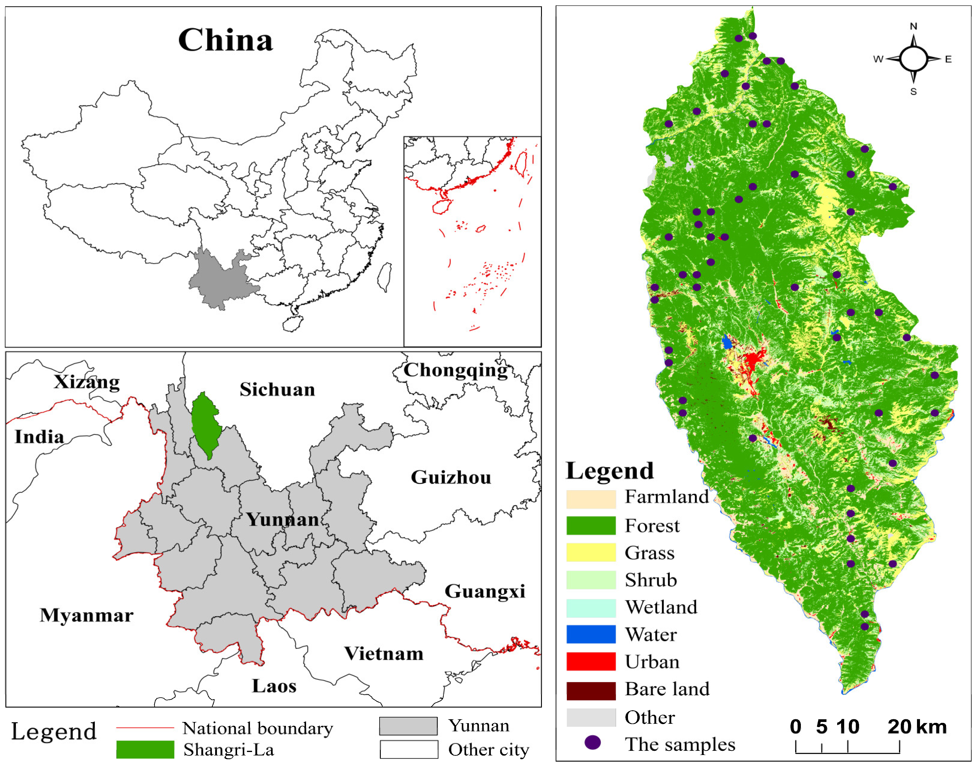
2.1. Study Area

Shangri-La is located between 99°20′~100°19′ E longitude and 26°52′~28°52′ N latitude at the confluence area of the Yunnan Province, the Sichuan Province, and the Tibet Autonomous Region. It lies in the northwestern part of the Yunnan Province, in the hinterland of the Hengduan Mountains on the southeastern edge of the Qinghai-Tibet Plateau. Its topography is undulating, with the lowest point is located in Luoji Township at 1503 meters, and the highest point located in the Balagzong Snow Mountain in Nixi Town at an altitude of 5545 meters. Due to it being located in a high altitude and low latitude area, the climate changes with the increase in altitude [22]. It encompasses six climate zones: the North subtropical valley, mountain warm temperate zone, mountain temperate zone, mountain cold temperate zone, high mountain subfrigid zone, and Alpine frigid zone. With 89.75 hectares of forest area and 78.6% of forest cover, Shangri-La is known for its dense forest cover. The primary wood species found in this region are Quercus aquifolioides, Picea likiangensis, Abies georgei, Pinus densata, and Pinus yunnanensis [23]. Figure 1 provides additional regional information about Shangri-La. Shangri-La has abundant forest resources. Quercus aquifolioides is one of the main dominant tree species, which is widely distributed and has a significant effect on the carbon balance in the region. Further, because the region is located on the edge of the Qinghai-Tibet Plateau, it has steep mountains, deep valleys, and the terrain is undulating. It is much challenging to accurately estimate forest carbon storage.

2.2. Ground Survey Data Collection and Processing

Our sample plots data were collected from the National Forestry Inventory in Yunnan in 2016, with a total of fifty-two sample plots, each with an area of (30 m × 30 m), distributed as shown in Figure 1. Each sample plot was recorded with a diameter at breast height, coordinates, canopy density, volume, and tree height [24]. In this study, the biomass of Quercus aquifolioides sample sites was calculated according to the model suggested in the industrial standard published by the State Forestry Administration. The model can be expressed using Equation (1). The product of individual plant biomass and the number of trees is the aboveground biomass of the small class. And the carbon storage is acquired by multiplying the biomass with carbon coefficients, as seen in Equation (2). Here, we set the carbon coefficients to 0.48, which was referenced by the Quercus aquifolioides industry standard [25]. The information on the carbon storage of Quercus aquifolioides in the observation point was obtained after calculation, as presented in

Table 1. Ground inventory sample information of Quercus aquifolioides.

Species	Sample Size	Minimum	Maximum	Average	SD
Quercus aquifolioides	52	5.36	131.98	41.79	30.23

; the maximum was 131.98 t/hm², and the minimum was 5.36 t/hm².

$${\mathrm{M}}_{\mathrm{Quercus}}=0.07806{\mathrm{D}}^{2.06321}{\mathrm{H}}^{0.57393}$$

(1)

C = M × C_C

(2)

where M is the aboveground biomass (kg/m²), D is the diameter at breast height (cm), H is the standing height (cm), C is the carbon storage (t/hm²), and C_C is the carbon conversion index.

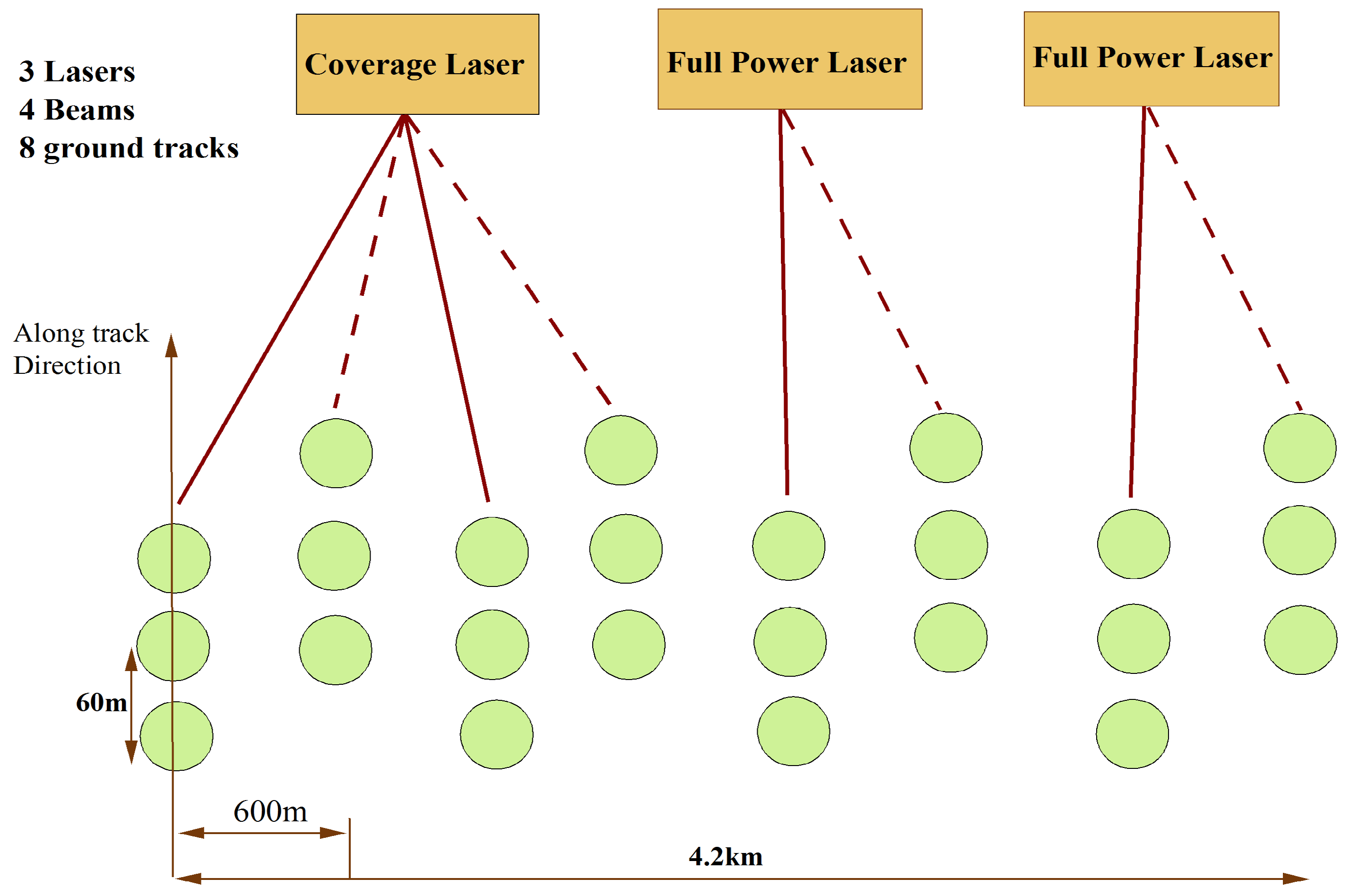
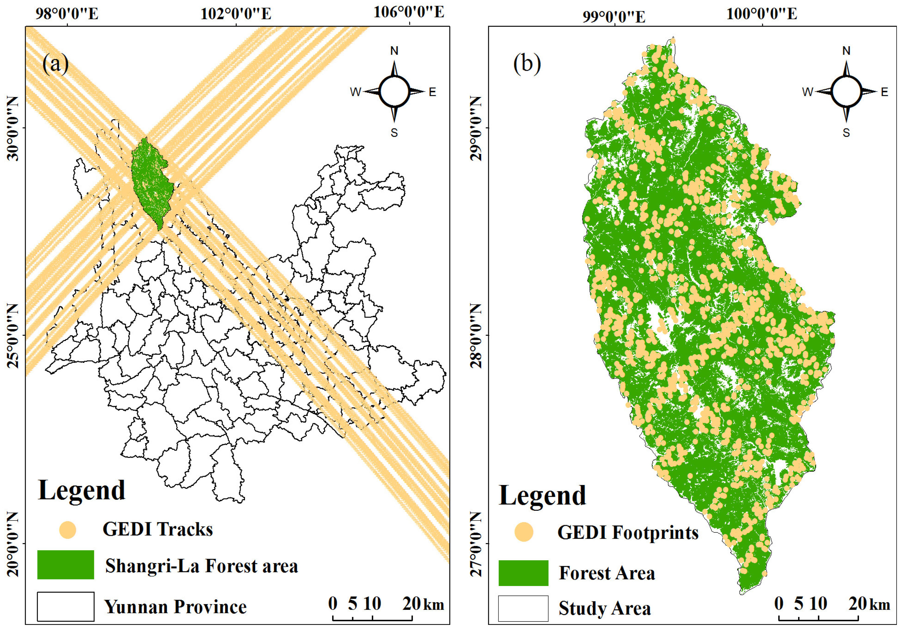
2.3. GEDI Data and Processing

The GEDI instrument, which is attached to the International Space Station (ISS), collects data globally between latitudes of 51.6° north and 51.6° south latitude. This data represent the highest resolution and largest sampling density in on-orbit optical detection and LiDAR instruments data [26]. The main objective is to enhance our ability to describe the impacts of climate change and land use on ecosystem structure and dynamics. The GEDI instrument consists of three lasers that are splitting and beam jittering, producing eight beam ground cross-sections at 600 meter intervals in the cross-orbit direction of the Earth’s surface. Each beam has footprint samples with a diameter of approximately 25 meters and an interval of about 60 meters along the track, covering a width of about 4.2 kilometers across the track [27]. Figure 2 illustrates the GEDI beam sampling mode [26]. This study used GEDI-derived Level 2B (L2B) data; it included eight beams and one metadata. The metadata contains comprehensive information, such as acquisition time, purpose, file name, and creation time. Additionally, each beam contains a total of one hundred and fifty-six fields that encompassed geographic location, land cover data, and more.

The GEDI data in this study can be download free from the Earthdata website (https://search.earthdata.nasa.gov/, accessed on 7 November 2022). Based on the vector boundary of Shangri-La, all beams in the study area are selected. There was a total of thirty-two GEDI orbit tracks data (Figure 3a), ranging from 23 April 2019 to 17 October 2019. At the same time, we used five indicators (quality_flag, degrade_flag, solar_elevation, leaf_off_flag, and sensitivity) to screen out high-quality, full-information light spots. If a value of quality_flag is 1, it meant that the waveform satisfies a specific criterion of high quality, so the footprints with a value of 1 were retained. A degrade_flag value of 1 demonstrated that the satellite was in orbit descent, and that the data were inaccurate. The sensitivity indicated the waveform penetrable to the largest tree covering in the canopy, with a value range from 0 to 1. When the data were closer to 1, it indicated high quality. Usually, the value was set to be greater than 0.95 in dense forest areas [28]. After quality filtering, 52,366 footprints were obtained (Figure 3b).

2.4. Landsat 9 and Data Processing

This study mainly used Landsat 9 optical remote sensing data, which can be processed and calculated through the Google Earth Engine (GEE) website platform (http://developers.google.cn, accessed on 7 May 2023). In this study, the GEE cloud removal algorithm was used to remove the cloud, and the image values corresponding to each pixel were obtained, followed by the extraction of the spectral band, vegetation indices, and other image feature parameters.

Landsat 9 was launched by USGS and NASA on 5 November 2021. After about 100 days of debugging, the data collected by Landsat 9 will be freely available to the world in early 2022 [29]. Landsat 9 is a near-polar sun-synchronous orbit satellite with an orbital height of 705 km, an orbital inclination of 98.2, a regression period of 16 days, a single scene width of 185 km, and a design life of five years. Landsat 9 is equipped with OLI-2 and TIRS-2 instruments, of which OLI-2 contains 9 bands with a spectrum spanning visible, near and mid-infrared, enabling monitoring of vegetation, coastal zone, aerosol, water vapor and, cloud [30]. Additionally, TIRS-2 contains two thermal infrared bands; it can satisfy the needs of thermal infrared radiation or thermal environment monitoring on the surface of the earth. The spatial resolution of bands 1 to 7 and 9 are 30 m, band 8 is 15 m, and bands 10 to 11 are 100 m. The Landsat 9 image includes Level-1 Precision Terrain (L1TP)-processed data and Level-2 data [31]. This research discusses the Landsat 9 Level 1T data in Shangri-La from March to May 2022 through GEE.

2.5. Characteristic Variables Extraction and Selection

Characteristic variables are the basis to estimate carbon storage, and the selection of appropriate variables can reduce redundancy, while raising the evaluation interpretability of the model. Characteristic variables which are commonly applied in carbon storage inversion include spectral variables and vegetation indices of optical remote sensing, and topographic factors.

2.5.1. Optical Remote Sensing Independent Variable Factors

Spectral variables mainly include band reflectance and vegetation indices. Vegetation indices, which reflect data on plant growth, coverage, and biomass, can distinguish vegetation from other ground objects [32]. These indices, which are calculated by band combining bands, provide a quantitative description of vegetation growth status. They have been broadly applied in vegetation classification, monitoring environmental changes and, crop yield estimation [33]. Considering the needs of this study and the characteristics of forest vegetation in Shangri-La, each band reflectance and ten vegetation indices were selected. The description and calculation equations of each vegetation index are shown in

Table 2. Formulas of the vegetation index.

Vegetation Index	Full Name	Expression
Band reflectance	B1-Coastal, B2-Blue, B3-Green, B4-Red, B5-NIR, B6-SWIR 1, B7-SWIR 2	-
NDVI	Normalized Difference Vegetation Index	NDVI = (NIR − R)/(NIR + R)
RVI	Ratio Vegetation Index	RVI = NIR/R
DVI	Difference Vegetation Index	DVI = NIR − R
RGVI	Red-green Vegetation Index	RGVI = (R − G)/(R + G)
GNDVI	Green Normalized Difference Vegetation Index	GNDVI = (NIR − G)/(NIR + G)
IPVI	Infrared Vegetation Index	IPVI = NIR/(NIR + R)
EVI	Enhanced Vegetation Index	EVI = (2.5 × (NIR − R))/(NIR + 6 × R − 7.5 × B + 1)
ARVI	Atmospherically Resistant Vegetation Index	ARVI = (NIR − (2 × R − B))/(NIR + (2 × R − B))
VARI	Visible atmospherically resistant Index	VARI = (G − R)/(G + R−B)

.

2.5.2. GEDI Parameters

Compared with GEDI L2A level data, L2B standard data products include additional vertical profile indicators such as total cover, total plant area volume density profile, directional gap probability profile, and foliage height diversity.

Table 3. Description of GEDI parameters.

Parameters	Description	Parameters	Description
cover	Total canopy cover	fhd_normal	Foliage height diversity index
pai	Total plant area index.	landsat_treecover	Landsat tree canopy cover
degrade_flag	Degrade flag	solar_elevation	Solar elevation
lon_lowestmode	Longitude of center of lowest mode	lat_lowestmode	Latitude of center of lowest mode
pgap_theta	Total gap between plant	modis_treecover	Percent tree cover from MODIS data
digital_elevation_model	Digital elevation model height above the WGS84 ellipsoid	modis_nonvegetated	Percent non-vegetated from MODIS data
leaf_off_doy	Leaf-off start day-of-year derived	leaf_on_doy	Leaf-on start day-of-year derived
rg	The ground energy value in the waveform	rv	The vegetation energy value in the waveform
rh100	Height above the ground at the start of the waveform signal	sensitivity	The waveform penetrable to the largest tree covering in the canopy
leaf_off_flag	Indicating if the observation was recorded under deciduous forest conditions	quality_flag	Flag simplifying selection of most useful data

contains fourteen modeling indices and six quality screening indices.

In addition to the vegetation indices extracted from the Landsat 9 images, as well as the canopy cover, leaf area index, and other factors provided by GEDI, this research also used topographic factors (elevation, slope, and aspect) to investigate the layout of Quercus aquifolioides carbon storage on various slopes and aspects.

2.6. Research Methods

In the early stage of this study, surface information was obtained using the Kriging interpolation method to interpolate the footprint parameters provided by GEDI. Then, the Landsat 9 image was coordinated with the GEDI parameters to analyze the correlation between each variable and carbon storage. And then, we used support vector machine, bagging regression, and random forest to build the carbon storage assessment model. The primary purposes of this analysis are as follows: (1) Finding the optimal semi-variance model of GEDI metrics. (2) Analyzing the correlation between vegetation indices and GEDI metrics and Quercus aquifolioides carbon storage. (3) Developing carbon storage estimation models and exploring the influence of explanatory variables on the accuracy of carbon storage estimation. (4) Estimating the carbon storage of Quercus aquifolioides and discussing its distribution characteristics on different slopes and aspects. The main steps can be seen in the technology roadmap (Figure 4).

2.6.1. Interpolation Method

• Variance Function

The variance function is also called the structure function, and one second of it is named as semi-variance. It is a basic tool and a special function of geostatistics. Variance function captures not only the structural variation in regionalized variables but also expresses their persistent variation. Modeling of variance function is a key environment between spatial description and prediction [34]. The variance function models are classified into abutment-valued models, abutment-free models, and pore effect models. In this study, we used the GS+ software to fit the optimal semi-variance model of each parameter.

$$\mathsf{\gamma }\left(\mathrm{h}\right)=\frac{1}{2N\left(h\right)}{\sum }_{i=1}^{N\left(h\right)}{\left[Z\left(x_i\right)-Z\left(x_i+h\right)\right]}^2$$

(3)

where $\mathsf{\gamma }$(h) is the variance function, $N\left(h\right)$ is the spatial separation distance between two points, $Z\left(x_i\right)$ and $Z\left(x_i+h\right)$ are the regionalized variables, and Z is the measured values at the spatial locations $x_i$ and $x_i+h$.

2.

Kriging Interpolation

The Kriging interpolation uses the structural features of sampled data and semi-variance functions of regionalized variables to provide unbiased estimation, and to determine the weighting coefficients at unsampled points according to minimum variance. And it is one of the most widely used interpolation methods. The data of other unmeasured positions are estimated using different sample data distributed in space [35].

$$Z_v^{*}\left(x_0\right)={\sum }_{i=1}^n{\lambda }_{i}Z\left(x_i\right)$$

(4)

where $x_i$ is the location of any point in the study area, and ${\lambda }_i$ is the weight factor. The Kriging equations are listed according to the unbiased and optimal conditions, and then the Kriging weight coefficient is obtained by calculating the Kriging equations. $Z_v^{*}(x_0)$ is the Kriging estimation results, $Z\left(x_i\right)$ is the sample points with known values, and n is the amount of GEDI footprints.

2.6.2. Carbon Storage Estimation Models

To compare the estimation accuracy of different models, this study selected three non-parametric models to establish carbon storage estimation models which combined the forest resource inventory data and characteristic variables. Three carbon storage models were used in this research (SVM, bagging, and RF).

• Support Vector Machine

A support vector machine, a supervised learning module related to learning algorithms, is used for data recognition and regression evaluation [36]. There exists certain performance differences in different SVM kernel functions. It maps the linearly inseparable data in the space to the high-dimensional feature space so that the data are separable in the feature space. Generally, three kernel functions are used to complete the multidimensional mapping from input space to feature space [37]. In this research, the ‘e1071’ package of R 4.2.3 was used to construct the SVR model and choose the RBF (radial basis function) as the kernel function. In order to obtain the best parameters, 10-fold cross-validation was used to optimize the mapping parameter (g) and penalty coefficient (c), with gamma set at 0.2 and C at 0.25.

2.

Bagging

Bagging is an algorithm that integrates different individuals into a learner. The basis of the bagging algorithm is to obtain different sample subsets via repeated sampling so that the learning tools trained on different sample subsets have a greater difference and a higher generalization performance. The bagging algorithm repeats sampling in each training set after extracting numerous training sets from the sample set of the sample plot using uniform sampling. After that, an experiment is conducted on this part of the sample and a decision tree is established, which is then combined with other decision trees [38]. The bagging function in the ‘ipred’ package of R 4.2.3 was used to model the samples in this study.

3.

Random Forest

Random forest is an important learning method for integration, which uses a decision tree as a bagging ensemble and randomly selects attributes in training. Its randomness is mainly reflected in the random selection of samples and the random selection of characteristic variables [39]. Random forest uses the boost strapping algorithm to randomly collect new datasets and put them back to extract 2/3 of samples from the original sample dataset. When used for regression, the mean of all decision tree forecasts is used as the final forecast value [40]. This study used the ‘randomforest’ package in R 4.2.3 to build the predictive model, and the most important parameters are the number of decision trees that built the sample size (ntree), and the number of random characteristics (mtry). According to 10-fold cross-validation, the optimal parameters ntree was 200, and mtry was 2. The importance of variables can be judged by analyzing the influence of variables on model mean square error and model tree node purity. This research sorted the importance of features using the % IncMSE in R software.

2.7. Evaluation of Model Accuracy

To minimize accidental errors resulting from splitting the training and test sets, this study used a ten-fold cross-validation method to split the dataset of fifty-two ground observation samples into training and validation sets. The principle of cross-validation involves dividing the dataset into ten groups of equal sample sizes. The other nine groups were utilized as the training set while one group was chosen consecutively as the verification set to test the model’s ability of estimation. For each cross-validation, the determination coefficient (R²) and root mean square error (RMSE) were calculated for the forecasted and realized values. This process was repeated ten times to calculate the average values [41]. A higher R² value indicated greater accuracy of the model, while a smaller RMSE value signified a more accurate regression model. The calculation of each indicator is as follows:

$${\mathrm{R}}^2=1-\frac{\sum _{i=1}^n{\left(y_i-{\widehat{y}}_i\right)}^2}{\sum _{i=1}^n{\left(y_i-\overline{y}\right)}^2}$$

(5)

$$\mathrm{RMSE}=\sqrt{\frac{\sum _{i=1}^n{\left(y_i-{\widehat{y}}_i\right)}^2}{n-1}}$$

(6)

where n is the sample size, $y_i$ is the actual carbon storage of the plot i, $\overline{y}$ is the mean of the measured carbon storage, and ${\widehat{y}}_i$ is the estimated value of carbon storage at plot i.

3. Results

3.1. Selection of Variance Function Models

In this research, the semi-variance function was fitted using four models through the GS+ 9.0 software and each parameter (nugget, sill, structural ratio, and range) was calculated in it. To ensure accuracy of the model, we selected the model with the highest R², smallest RSS, and largest structure ratio as the optimal semi-variance function model.

The model parameters obtained via GS + fitting semi-variance are listed in

Table 4. Results of variance function of all models.

Parameter Name	Model	R2	Residual SS	Nugget	Sill	Structural Ratio	Range
digital_elevation_model	Linear	0.97	5.75 × 109	158,182.97	492,097.45	0.68	0.93
	Spherical	0.96	6.02 × 109	151,000.00	647,400.00	0.77	1.91
	Exponential	0.95	7.56 × 109	130,000.00	671,000.00	0.81	2.86
	Gaussian	0.94	9.80 × 109	195,000.00	539,300.00	0.64	1.20
modis_treecover	Linear	0.41	1.82	4.66	5.60	0.17	0.93
	Spherical	0.60	1.23	0.18	5.24	0.97	0.07
	Exponential	0.72	0.88	0.61	5.28	0.88	0.11
	Gaussian	0.60	1.23	0.74	5.24	0.86	0.06
fhd_normal	Linear	0.06	5.30 × 10−3	0.35	0.36	0.04	0.93
	Spherical	0.44	3.18 × 10−3	0.02	0.36	0.95	0.06
	Exponential	0.42	2.94 × 10−3	0.04	0.36	0.89	0.07
	Gaussian	0.44	3.18 × 10−3	0.06	0.36	0.84	0.05

. The results indicated that each parameter extracted from the GEDI had an intense spatial correlation and was suitable for the Kriging spatial interpolation analysis. Specifically, the linear model with digital_elevation_model, modis_treecover, and fhd_normal as well as the Gaussian model of digital_elevation_model had a structure ratio below 75%, while the structure ratio of each model of the remaining variables was above 80%. We selected the spherical model for the digital_elevation_model as the best variance function model on the basis of the rule that the greater the R², the smaller the RSS. Additionally, the exponential model exhibited the best fitting effect in the case of modis_treecover and fhd_normal, with the largest R², smallest RSS, and largest structure ratio. Therefore, the exponential model was chosen as the logical variance model for these two parameters.

3.2. Variable Correlation Analysis

In this study, a total of thirty-three characteristic variables were obtained, including fourteen vegetation vertical structure characteristics data from GEDI, nine vegetation indices and seven band reflectances from Landsat 9, and three topographic factors (slope, aspect, and elevation).

To analyze the interaction between different remote sensing characteristics and Quercus aquifolioides carbon storage as well as to compare the estimation accuracy of different regression models, Pearson correlation analysis was carried out between the remote sensing characteristic factors extracted from GEDI and Landsat 9 images and the Quercus aquifolioides carbon storage in the sample sites using R software. The correlation coefficient matrix was displayed in Figure 5. The Pearson correlation coefficient between remote sensing variables and carbon storage ranged from −0.228 to 0.307, with five variables significantly associated with carbon storage (p < 0.05). Among these variables, digital_elevation_model, modis_treecover, dem, fhd_normal, and B1 had the highest correlation coefficients with carbon storage (0.307, 0.254, 0.234, −0.228, and 0.217, respectively).

The band composition of Landsat 9 remote sensing variables shows that the sensitivity of vegetation indices composed of each band to carbon storage was low, while the sensitivity of single band reflectance was relatively high. In addition, digital_elevation_model, modis_treecover, and fhd_normal were significantly positively correlated to carbon storage, indicating that the waveform data provided by GEDI contained information affecting vegetation carbon storage. The remaining variables related to topography and vegetation, such as the atmospherically resistant vegetation index (ARVI), the visible atmospherically resistant index (VARI), the integration of vegetation components in the waveform (rv), and the height from the beginning of the received waveform signal (rh100), also contributed to the evaluation of carbon storage, but the effect was not significant.

The importance of each variable was ranked via random forest (Figure 6). The brown line is the connecting line of the %incMSE value of each variable. Because % IncMSE is verified by OOB data, and the reliability of feature selection is high. Therefore, this paper chose the results of % IncMSE for feature selection. By combing Pearson correlation analysis, the characteristic variables that were significantly correlated at the 0.05 level were screened. Finally, six characteristic variables of digital_elevation_model, DEM, EVI, B1, modis_treecover, and fhd_normal were selected as the modeling factors.

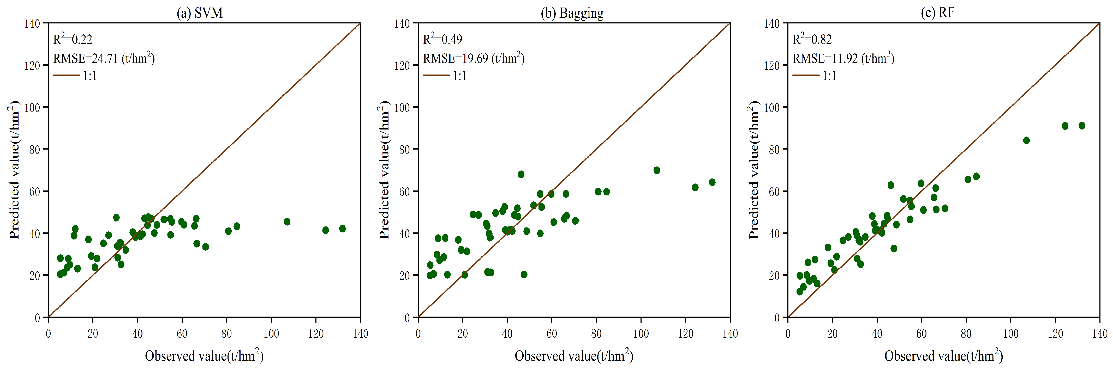
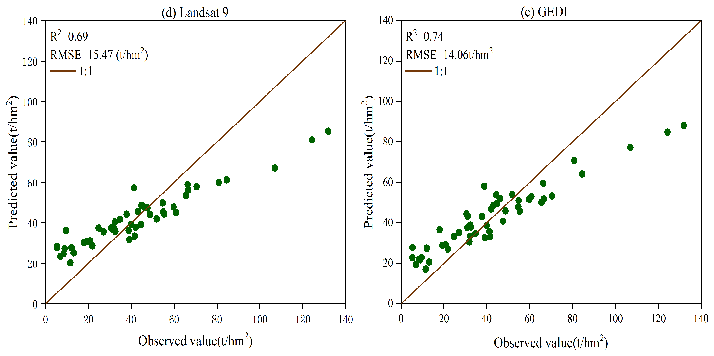
3.3. Comparison of Carbon Storage Estimation Results

The appropriate combination of independent variables derived from GEDI L2B spaceborne LiDAR data and Landsat 9 remote sensing images was selected by screening individual factors using random forest and Pearson correlation coefficient analysis. Model building for the selected variables and observed carbon storage was conducted using SVM, bagging, and RF, and the accuracy of each model was evaluated. Two indicators, R² and RMSE, were used to compare and analyze the prediction outcomes of various models, and the findings are presented in Figure 7a–c.

Comparing the R² and RMSE of the three models, it was found that RF had the highest estimation accuracy with an R² of 0.82 and RMSE of 11.92 t/hm². The bagging model had moderate evaluation precision, wherein the R² was 0.49 and RMSE was 19.69t/hm². In contrast, the SVM model had the worst results; the R² was 0.49 and RMSE was 23.97 t/hm². The results revealed that in the model established via SVM, the sample sites were discretely spread on each edge of the 1:1 line, and the fitting degree of the model was not high, while the random forest model had a higher precision in evaluating carbon storage. And the distribution of samples was more concentrated, and the estimation error was smaller when the carbon storage was higher or lower. In order to compare the accuracy difference of single remote sensing data source and joint multi-source remote sensing data to estimate carbon storage, we conducted feature optimization of variables extracted from GEDI and Landsat 9 images. Rv, sensitivity, modis_treecover, rh100, and landsat_treecover were selected in GEDI, while B7, VARI, B4, RGVI, and IPVI were selected in Landsat 9. The results are shown in Figure 7d,e, which were modeled via random forest. When only the variable of Landsat 9 was used, the R² was 0.69, RMSE was 15.38 t/hm² and the estimated average value was 37.18 t/hm². But the R² was 0.74, RMSE was 14.06 t/hm² and the average carbon storage was 38.09 t/hm² if only the variable of GEDI was used. These results demonstrated that the estimation results of carbon storage using GEDI or Landsat 9 alone were not as accurate as the estimation results of integrating GEDI and Landsat 9.

3.4. Spatial Distribution of Carbon Storage in Shangri-La

Using GEDI and Landsat 9 images for the primary data supplied with the combination of Shangri-La Quercus aquifolioides sample plot, a random forest model has been applied to predict the carbon storage. The carbon storage distribution is shown in Figure 8, which revealed that the carbon storage of Quercus aquifolioides in Shangri-La ranged from 8.22 t/hm² to 94.63 t/hm², with a total carbon storage of approximately 5,374,137.62 t, and an average of 42.44 t/hm². The high-value area and low-value area of carbon storage are staggered in the whole study area, with uneven distribution and large regional differences. As shown in Figure 7, the carbon storage and biomass of Quercus aquifolioides in Shangri-La had a uniform spatial composition. The areas with the upper value were primarily located in the southeast of Shangri-La, including the north of Luoji Township, the mountains surrounding the Luzila Snow Mountain, the southwest of Baha Snow Mountain, the junction of the mountains in Geza Township and Dongwang Township in the north, and the mountains around the Balagzong Grand Canyon in Nixi Township. These areas, classified as alpine-gorge regions with elevations ranging between 3000 and 4000 m, exhibited abundant Quercus aquifolioides resources and had high carbon storage. Conversely, the low-value areas were located predominantly situated in the southwest of Xiaozhongdian Town, the north of Tiger Leaping Gorge Town, and the Valley of Dongwang Township. These areas were characterized by valley terrain, with lower slopes and lower elevations. Due to the sparse distribution of Quercus aquifolioides species at lower altitudes and gentle slopes, the carbon storage value in these regions was comparatively lower than in other areas.

3.5. Distribution Regularity of Quercus aquifolioides Carbon Storage in Different Aspect

After model estimation, we found that the overall carbon storage of Quercus aquifolioides in Shangri-La was 5,374,137.62 t, and the average value was 42.44 t/hm². After classifying the distribution area of Quercus aquifolioides in Shangri-La, we divided the study area into flat (0°), east (67.5~112.5°), southeast (112.5~157.5°), south (157.5~202.5°), southwest (202.5~247.5°), west (247.5~292.5°), northwest (292.5~337.5°), north (0~22.5°, 337.5~360°), and northeast (22.5~67.5°), which represented flat, half-shady slope, half-sunny slope, sunny slope, sunny slope, half-sunny slope, half-shady slope, shady slope, and shady slope, respectively. The spatial analysis method was used to extract the carbon storage of Quercus aquifolioides on different aspects and slopes in ArcGIS 10.2. The carbon storage of Quercus aquifolioides on different aspects is shown in Figure 9. It was observed that carbon storage was predominantly distributed in the sunny slope, which was 2,117,318.33 t, and it accounted for 39.43% of the total area. Next, the amount of the half-sunny was 1,411,515.03 t which contained about 26.29% of the carbon storage in Shangri-La, and distribution in flat slope was the least, which was 332,645.93 t, just accounting for only 6.19% of all carbon storage. Overall, the distribution pattern of Quercus carbon storage in Shangri-La followed the sequence of sunny slope, half-sunny slope, half-shady slope, and shady slope. This pattern was consistent with the characteristics of Quercus aquifolioides forests in Yunnan, Guizhou, Sichuan, and Tibet, which were mainly found on mountain slopes at altitudes of 2000~4500 m with abundant sunlight.

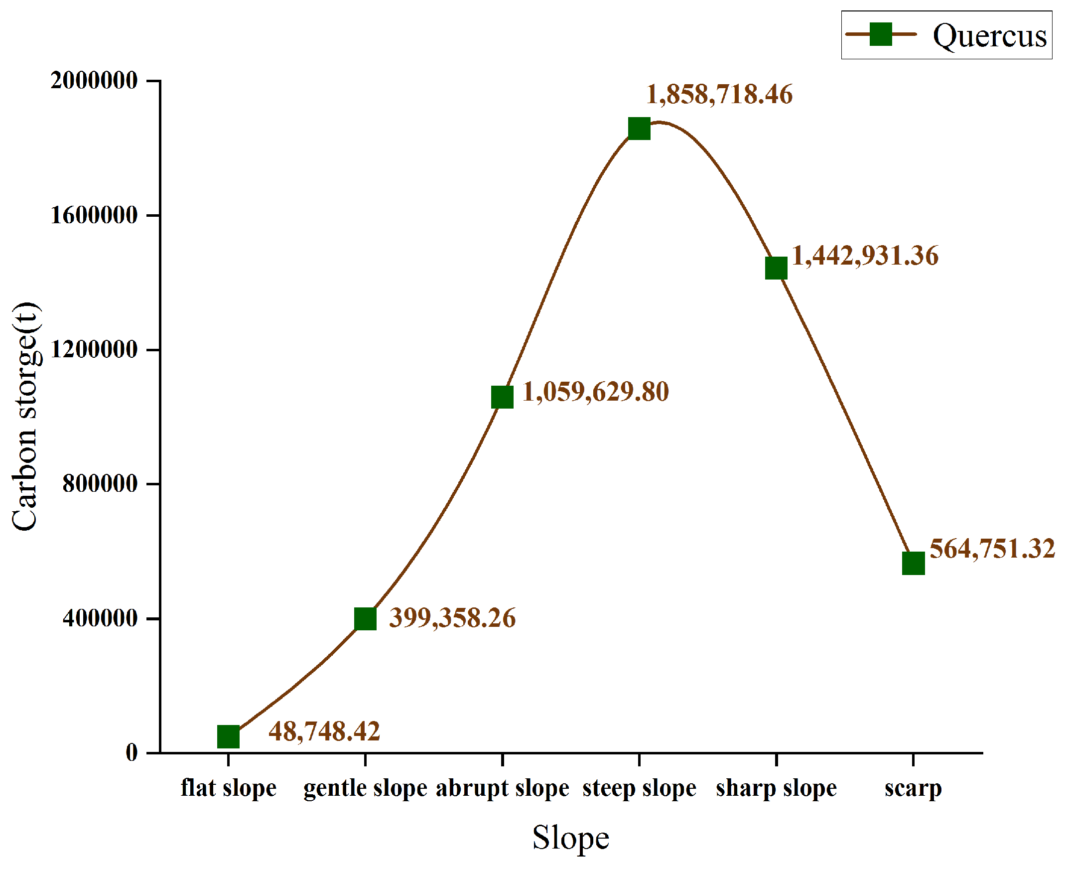
3.6. Distribution Regularity of Quercus aquifolioides Carbon Storage in Different Slopes

According to organized survey data, the study area was divided into flat slope (<5°), gentle slope (5~15°), abrupt slope (15~25°), steep slope (25~35°), sharp slope (35~45°) and scarp (>45°). As shown in Figure 10, the carbon storage of Quercus aquifolioides in the flat slope was the lowest, which was 48,748.42 t, accounting for only 0.91% of the total Quercus aquifolioides carbon storage. But the value in the steep slope was 1,858,718.46 t; it was the largest compared with other slopes, which was about 34.59% of all carbon storage. And the second highest was the sharp slopes, with 26.85% of the total value. In general, the distribution pattern of Quercus carbon storage in Shangri-La followed the sequence of the steep slope, sharp slope, abrupt slope, scarp, gentle slope, and flat slope. Furthermore, the altitude of Shangri-La Quercus aquifolioides ranged from 1451 to 5314 meters. Previous studies have shown that Quercus aquifolioides was most abundant at altitudes of 2500 m to 3000 m, reaching up to 93.75% of the total area. The carbon storage of Shangri-La Quercus aquifolioides was mainly concentrated in high-altitude areas, with the highest values observed on steep slopes and sharp slopes. This distribution pattern aligned with the characteristics of higher altitudes and steeper slopes.

4. Discussion

The demands for high-precision, high-resolution, and large-scale carbon storage estimation are increasing. And a signal remote sensing resource no longer satisfied the requirement of large-scale accurate estimation of carbon storage. Optical remote sensing was easily influenced by “saturation effects”, and the climate condition increased the difficulties in obtaining microwave remote sensing. Although spaceborne LiDAR can provide vertical structure information of vegetations, the result was discontinuous in space. Integrating multi-source remote sensing data, such as GEDI, ICESat-2, Landsat, and Sentinel, provided a new research direction for researchers. The key challenge in estimating forest structural characteristics using GEDI spaceborne LiDAR data combined with medium-resolution satellite images is to solve the problem of discontinuous distribution of GEDI footprints and the mismatch between GEDI and other image resolutions. Therefore, this study aimed to address these challenges and estimate the precision and accuracy of carbon storage by integrating GEDI spaceborne LiDAR and Landsat 9 optical satellite data. By providing a potential solution to the issue of partial coverage of GEDI spaceborne LiDAR footprints, this method had great potential for estimating forest carbon storage at the county scale and demonstrated the possibility of wide-scale applications.

4.1. Verifying Carbon Storage Estimation

The value of Quercus aquifolioides in forest resource inventory in 2016 was used as ground observed data; the Quercus aquifolioides volume in Shangri-La was found to be 4.04% after calculating and summarizing the data of previous studies [42]; the 3-year growth rate was multiplied with the 2016 observed volume accumulation to obtain the total volume and then the volume–biomass conversion model was used to deduce the amount of total biomass of Quercus aquifolioides in 2019. Finally, the measured carbon storage of Quercus aquifolioides in 2019 was found to be 5,879,608.28 t after multiplying the biomass with 0.48. This result was in the same order compared with the value combined with Landsat 9 optical remote sensing and GEDI LiDAR estimation (total carbon storage was about 5,374,137.62 t, with an average of 42.44 t/hm²).

Previous research also estimated carbon storage in Shangri-La based on remote sensing technology. Wang et al. [43] used a standing tree biomass model and carbon measurement parameters. Based on the forest resources inventory and planning data in Shangri-La, the average diameter at breast height, average tree height, and tree number of dominant tree species in each small class of forest were used to estimate the carbon storage of tree forest; the value of Quercus aquifolioides was 6,453,486 t, and the average value was 51.54 t/hm². Cheng et al. [44] used TM remote sensing as a data resource, combined with climate, temperature, humidity, and topography data. The carbon storage and density distribution of forest plant communities (soil layer, tree layer, shrub layer, litter layer, and herb layer) were estimated via the multivariate regression model, the BP neural network model, and the remote sensing information model. Finally, the carbon storage of Quercus aquifolioides was estimated to be 8,179,695.73 t. There were certain errors in the estimated carbon storage of Quercus aquifolioides calculated via the traditional models and optical remote sensing by Wang and Cheng et al. compared with the ground truth value. All their results overestimated Quercus aquifolioides carbon storage. However, our estimated results that integrated GEDI L2B Spaceborne LiDAR and Landsat 9 optimal remote sensing were closer to the measured value, which demonstrated that the combination of multiple data sources not only compensated for the saturation problem of optical remote sensing in high-value and low-value areas but also fully utilized the forest vertical structure information obtained via LiDAR.

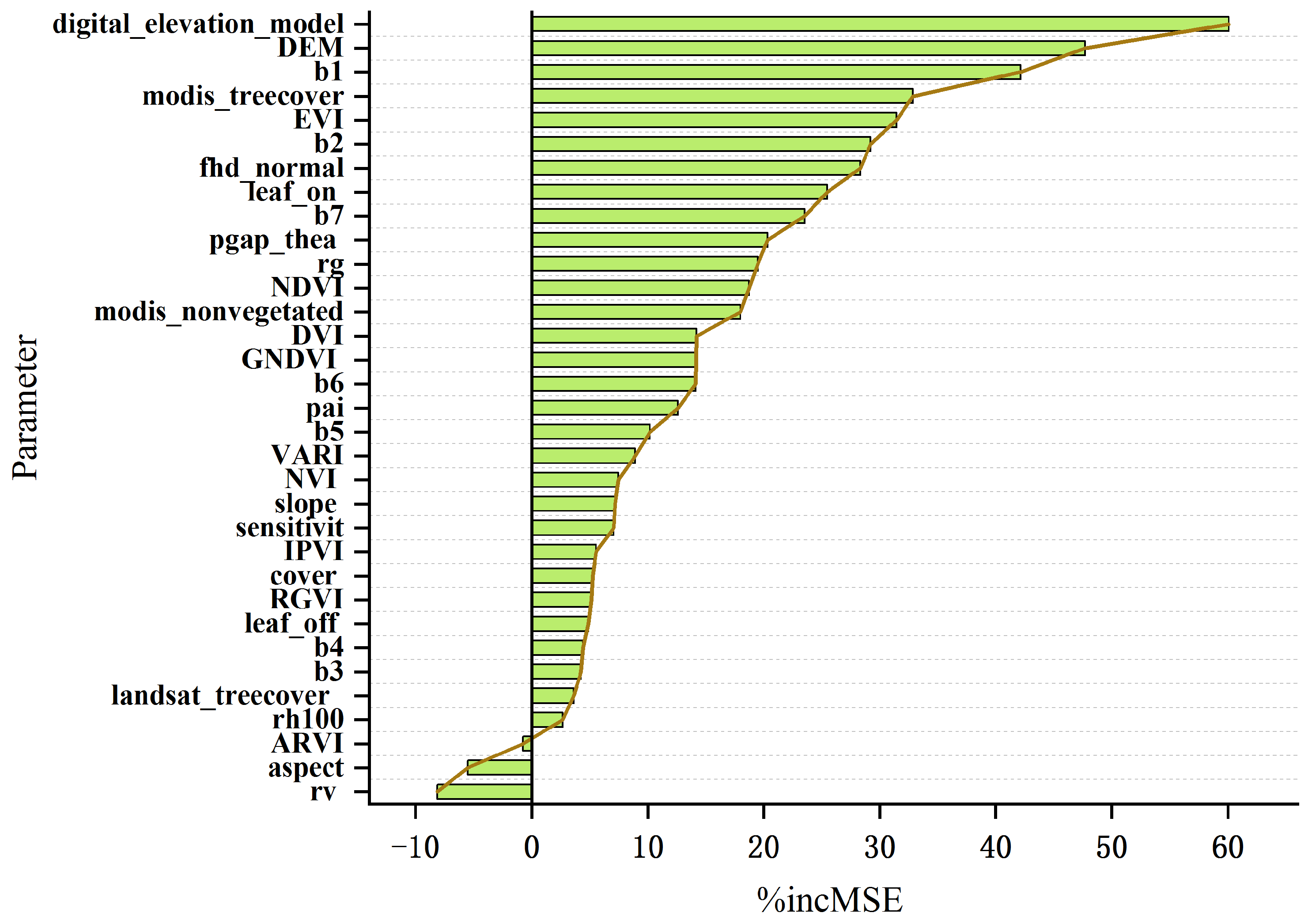
4.2. The Impact of Variable Selection on the Accuracy of Carbon Storage Estimation

A common limitation of optimal sensors is that they cannot accurately capture changes in aboveground biomass and carbon storage. They can measure three-dimensional forest structure, but cannot obtain three-dimensional forest structure information. In this study, GEE was used to acquire pre-processed Landsat 9 images. Images with less than 2% cloud cover in the vegetation growing season (March to May) in 2022 were obtained. Previous studies have shown that the application of different feature combinations can effectively avoid the loss of information caused when using a single variable model and it also can determine the range of AGB saturation points based on different data [45]. To analyze the influence of different variables selection on carbon storage estimation results, we conducted a feature optimization of variables extracted from the GEDI and Landsat 9 images, as seen in Figure 7d,e. The estimation results of this study were similar to Jiao’s (who used regression with log transformations model to integrate the Sentinel-2 and GEDI image feature variables, wherein the estimated R² was 0.72 and the RMSE was 17.93 t/hm²) [46]. The results illustrated that the accuracy of carbon storage inversion using optical images or spaceborne LiDAR variables alone was lower than that of estimation by integrating multiple data sources.

According to the results of the estimation model, combined with the characteristics of optical information and the calculation method of sample carbon storage, it can be seen that optical remote sensing can only obtain the reflection or radiation information of the vegetation surface. It had some limitations in estimating carbon storage. But the spaceborne LiDAR had the ability to acquire forest vertical structure information, resulting in better estimation accuracy for Quercus aquifolioides carbon storage compared to optical remote sensing data. Hence, the combination of the two information sources reflected the characteristics of carbon storage from both canopy and vertical structures, so as to achieve complementary information and improve the estimation accuracy of carbon storage [47]. In consideration of the feature variables, we just chose one vegetation index (EVI) and one band reflectance (B1) to build the model, because the research suggested that vegetation indices sensitivity is reduced in areas with dense vegetation [48]. Consequently, the correlation between vegetation indices and Quercus aquifolioides carbon storage was lower than other feature variables. Moreover, this study discovered a strong correlation between different vegetation indices, which results in multicollinearity between variables and affected both the correlation between vegetation indices and biomass, as well as the results of random forest feature selection. Therefore, a collinearity diagnosis of the vegetation index extracted from Landsat 9 in SPSS 26 was performed, and some vegetation indices variables with strong collinearity were eliminated to reduce estimation errors.

4.3. The Influence of Different GEDI Algorithm Setting Groups for the Carbon Storage Estimation Accuracy

The estimation results of forest canopy height and biomass using spaceborne LiDAR can be affected by adverse conditions such as low-energy ground reflection or high background noise. For different canopy and ground scenes, at the same time, in order to reduce those unfavorable conditions and consider the difference between daytime and night, GEDI set six different combinations of noise threshold, signal threshold, start threshold, and end threshold for users to choose, as shown in

Table 5. GEDI algorithm setting groups.

Algorithm Setting Group	Smoothing Width (Noise)	Smoothing Width (Signal)	Waveform Signal Start Threshold	Waveform Signal end Threshold
1	6.5σ	6.5σ	3σ	6σ
2	6.5σ	3.5σ	3σ	3σ
3	6.5σ	3.5σ	3σ	6σ
4	6.5σ	6.5σ	6σ	6σ
5	6.5σ	3.5σ	3σ	2σ
6	6.5σ	3.5σ	3σ	4σ

σ means the standard deviation of the background noise level.

. Different setting groups achieved the purpose of controlling the waveform length by changing the waveform signal smoothing width, signal start threshold, and signal end threshold [49]. Setting group 1 was typically used for most cases, while other setting groups were designed to provide accurate information when observation conditions were not good.

In order to obtain a more accurate forest canopy height, Potapov et al. [50] obtained the final forest canopy height by removing the maximum and minimum values in the six algorithms and then by averaging them. Compared with airborne LiDAR data, it showed that different GEDI algorithm setting groups in different environments will affect the measurement accuracy of GEDI. Liu et al. [51] compared different algorithms for varying vegetation coverage and selected the optimal algorithm based on different degrees of coverage. The results indicated that algorithm four worked best for plant density less than 0.2, algorithm two for vegetation coverage above 0.8, and algorithm one is more accurate for the remaining coverage than the others. Han et al. [52] verified six groups of data with airborne data, and the precision of six algorithm sets of elevation data inversion of max canopy height of GEDI L2A was analyzed. At the same time, the accuracy of estimating forest biomass was calculated for seven algorithm groups of L4A biomass products. The results showed that among the six algorithm settings of GEDI L2A, the lowest estimation accuracy was that of algorithm five, and the highest accuracy was that of algorithm four. When using L4A data to evaluate biomass, the algorithm two group had the highest accuracy among the seven algorithm groups.

The different algorithms had a certain influence on GEDI accuracy under different environments. Although GEDI L2B did not involve specific algorithm setting groups, some parameters (such as rg, pgap_thea, rv, and rx_enrgry) in L2B were designed by the selected L2A algorithm or others corresponding to different L2A processing algorithms. To compensate for the lack of airborne LiDAR data in verifying the accuracy of GEDI algorithm setting groups, therefore, this study selected the L2B parameters under the default algorithm for Kriging interpolation to obtain surface information. Future research will focus on analyzing the accuracy of various GEDI algorithm groups when estimating carbon storage in Shangri-La according to different forest types, surface slopes, and vegetation coverage, and to find the algorithm group with the highest estimation precision under different conditions.

4.4. Limitations and Prospects

GEDI footprints were not continuous, and in order to solve this problem and obtain the GEDI parameter information in entire Shangri-La, the Kriging method was used to interpolate footprints information into the polygon. The footprint of the spaceborne LiDAR is evenly distributed along the track. Usage of single spaceborne LiDAR interpolation mainly displays an intensive strip effect across ground tracks. Therefore, before interpolation, we carried out a screening of all footprints in the study area according to the filtering principle. The poor-quality footprints on one strip or adjacent strips were deleted to enhance the spatial randomness. However, the remaining footprints still cannot fully meet the spatial random distribution. Previous research demonstrated that increasing the footprints from other spaceborne LiDAR may solve the problem that the stripe effect of spatial interpolation creates [53]. Therefore, future research can consider combining the footprints of another LiDAR sensor, such as ICESat-2; combining two sensor data will allow to disrupt the phenomenon wherein homogeneous distribution of footprints from a single sensor weaken the strip effect during spatial interpolation.

At the same time, due to a lack of verification data from airborne LiDAR, we cannot verify the accuracy of the GEDI L2B parameters under different algorithm setting groups. Therefore, this study relied on the default algorithm settings to obtain the GEDI parameters. Future research can develop some custom algorithms to decompose the original GEDI L1B waveform and acquire high-precision parameters of the forest vertical structure. Rather than using the default values provided in the standard GEDI L2B data product, a special algorithm can be tailored to different terrain conditions, regions, forest types, and vegetation coverage [54]. Combined with spaceborne LiDAR and optical remote sensing data, the synthesis of multiple variables provided rich information and it also offered more possibilities for finding the correlation between remote sensing images and Quercus aquifolioides sample data. However, the combination of different remote sensing data sources, with variations in sensors, time resolutions, spectral resolutions, and radiation resolutions, will cause some effect on the precision of the models [55]. The diameter of the GEDI footprint level was 25 meters, but the resolution of the Landsat 9 optical remote sensing image was 30 meters. Therefore, the integration of remote sensing images with different resolutions was a major problem to be solved in this study. To overcome this challenge, based on the surface information obtained by the interpolation of GEDI footprints variable data, the spatial resolution of the surface GEDI parameters was resampled to 30 m when the raster data were exported, which was unified with the resolution of Landsat 9. In future research, GEDI data can be integrated and estimated with other data sources, such as MODIS and Sentinel, at a unified resolution.

5. Conclusions

In this study, remote sensing data from two different sensors, the new generation LiDAR GEDI and the land monitoring satellite Landsat 9, were combined to estimate the carbon storage of the Quercus aquifolioides forest ecosystem in Shangri-La. Our study proposed that the parameters of GEDI footprints are to be interpolated to the surface via the Kriging interpolation to solve the problem of GEDI data discontinuity. The results show that the digital_elevation_model, modis_treecover, and fhd_normal provided by GEDI, and EVI and B2 offered by Landsat 9 had a high correlation with Quercus aquifolioides carbon storage. And the random forest had the highest accuracy amongst the three models (R² = 0.81 and RMSE = 11.92 t/hm²). We discovered a consistent agreement between the evaluated results assessed by integrating GEDI and Landsat 9 (5,374,137.62 t) and the observed values calculated by the National Forestry Inventory (5,879,608.28 t). Through the analysis of the carbon storage of Quercus aquifolioides in different aspects and slopes, the carbon storage distributed on the steep slopes (25~35°) and the sunny slopes (202.5~292.5°) were found to be the largest. Our study demonstrated that combining GEDI LiDAR and optical remote sensing Landsat 9 to estimate the carbon storage in Shangri-La can provide a reference for multi-source remote sensing inversion at the county scale by integrating multiple data.

References

1. Shao, W.; Cai, J.; Wu, H.; Liu, J.; Zhang, H.; Huang, H. An Assessment of Carbon Storage in China’s Arboreal Forests. Forests 2017, 8, 110. [Google Scholar] [CrossRef]
2. Zhao, N.; Zhou, L.; Zhuang, J.; Wang, Y.; Zhou, W.; Chen, J.; Song, J.; Ding, J.; Chi, Y. Integration analysis of the carbon sources and sinks in terrestrial ecosystem, China. Acta Ecol. Sin. 2021, 42, 7648–7658. [Google Scholar] [CrossRef]
3. Luo, Y.; Keenan, T.F.; Smith, M. Predictability of the terrestrial carbon cycle. Glob. Chang. Biol. 2015, 21, 1737–1751. [Google Scholar] [CrossRef] [PubMed]
4. Amir, S.; Hormoz, S.; Scott, P.; Shaban, S. A comparative assessment of multi-temporal Landsat 8 and machine learning algorithms for estimating aboveground carbon stock in coppice oak forests. Int. J. Remote Sens. 2017, 38, 6407–6432. [Google Scholar] [CrossRef]
5. Kaisheng, L. Spatial Pattern of Forest Carbon Storage in the Vertical and Horizontal Directions Based on HJ-CCD Remote Sensing Imagery. Remote Sens. 2019, 11, 788. [Google Scholar] [CrossRef]
6. Long, Y.; Jiang, F.G.; Sun, H.; Wang, T.H.; Zou, Q.; Chen, C.S. Estimating vegetation carbon storage based on optimal bandwidth selected from geographically weighted regression model in Shenzhen City. Acta Ecol. Sin. 2022, 42, 4933–4945. [Google Scholar] [CrossRef]
7. Yan, E.; Lin, H.; Wang, G.; Sun, H. Improvement of Forest Carbon Estimation by Integration of Regression Modeling and Spectral Unmixing of Landsat Data. IEEE Geosci. Remote Sens. Lett. 2015, 12, 2003–2007. [Google Scholar] [CrossRef]
8. Zhang, J.; Benoit, R.; Arturo, S.; Karen, C. Intra-and inter-class spectral variability of tropical tree species at La Selva, Costa Rica: Implications for species identification using HYDICE imagery. Remote Sens. Environ. 2006, 105, 129–141. [Google Scholar] [CrossRef]
9. Svein, S.; Rasmus, A.; Terje, G.; Erik, N.; Dan, J.W. Estimating spruce and pine biomass with interferometric X-band SAR. Remote Sens. Environ. 2010, 114, 2353–2360. [Google Scholar] [CrossRef]
10. Xi, Z.L.; Xu, H.; Xing, Y.; Gong, W.; Chen, G.; Yang, S. Forest Canopy Height Mapping by Synergizing ICESat-2, Sentinel-1, Sentinel-2 and Topographic Information Based on Machine Learning Methods. Remote Sens. 2022, 14, 364. [Google Scholar] [CrossRef]
11. Jiang, F.; Deng, M.; Tang, J.; Fu, L.; Sun, H. Integrating spaceborne LiDAR and Sentinel-2 images to estimate forest aboveground biomass in Northern China. Carbon Balance Manag. 2022, 17, 12. [Google Scholar] [CrossRef]
12. Svetlana, S.; Sören, H.; Sean, P.H.; Hans-Erik, A.; Hans, P.; Wilmer, P.; Paul, L.P.; Erik, N.; Timothy, G.; Göran, S. Generalized Hierarchical Model-Based Estimation for Aboveground Biomass Assessment Using GEDI and Landsat Data. Remote Sens. 2018, 10, 1832. [Google Scholar] [CrossRef]
13. Duncanson, L.; Neuenschwander, A.; Hancock, S.; Thomas, N.; Fatoyinbo, T.; Simard, M.; Silva, C.A.; Armston, J.; Luthcke, S.B.; Hofton, M.; et al. Biomass estimation from simulated GEDI, ICESat-2 and NISAR across environmental gradients in Sonoma County, California. Remote Sens. Environ. 2020, 242, 111779. [Google Scholar] [CrossRef]
14. Dorado-Roda, I.; Pascual, A.; Godinho, S.; Silva, C.A.; Botequim, B.; Rodríguez-Gonzálvez, P.; González-Ferreiro, E.; Guerra-Hernández, J. Assessing the Accuracy of GEDI Data for Canopy Height and Aboveground Biomass Estimates in Mediterranean Forests. Remote Sens. 2021, 13, 2279. [Google Scholar] [CrossRef]
15. Kanmegne, T.D.; Latifi, H.; Ullmann, T.; Baumhauer, R.; Bayala, J.; Thiel, M. Estimation of Aboveground Biomass in Agroforestry Systems over Three Climatic Regions in West Africa Using Sentinel-1, Sentinel-2, ALOS, and GEDI Data. Sensors 2022, 23, 349. [Google Scholar] [CrossRef]
16. Shendryk, Y. Fusing GEDI with earth observation data for large area aboveground biomass mapping. Int. J. Appl. Earth Obs. 2022, 115, 103108. [Google Scholar] [CrossRef]
17. Silva, C.A.; Duncanson, L.; Hancock, S.; Neuenschwander, A.; Thomas, N.; Hofton, M.; Fatoyinbo, L.; Simard, M.; Marshak, C.Z.; Armston, J.L.; et al. Fusing simulated GEDI, ICESat-2 and NISAR data for regional aboveground biomass mapping. Remote Sens. Environ. 2021, 253, 112234. [Google Scholar] [CrossRef]
18. Liu, L. Inversion of Forest Canopy Height in Yunnan Province Based on Spaceborne Lidar Data and Optical Remote Sensing Data. Master’s Thesis, Yunnan Normal University, Kunming, China, 2022. [Google Scholar] [CrossRef]
19. Sothe, C.; Gonsamo, A.; Lourenço, R.B.; Kurz, W.A.; Snider, J. Spatially Continuous Mapping of Forest Canopy Height in Canada by Combining GEDI and ICESat-2 with PALSAR and Sentinel. Remote Sens. 2022, 14, 5158. [Google Scholar] [CrossRef]
20. Pascual, A.; Guerra-Hernández, J.; Armston, J.; Minor, D.M.; Duncanson, L.I.; May, P.B.; Kellner, J.R.; Dubayah, R. Assessing the performance of NASA’s GEDI L4A footprint aboveground biomass density models using National Forest Inventory and airborne laser scanning data in Mediterranean forest ecosystems. For. Ecol. Manag. 2023, 538, 120975. [Google Scholar] [CrossRef]
21. Zeng, C.; Wang, L. The characteristics and application prospects of the new generation Landsat satellite constellation. Urban Geotech. Investig. Surv. 2022, 5, 78–85. [Google Scholar]
22. Li, C.; Chen, D.; Wu, D.; Su, X. Design of an EIoT system for nature reserves: A case study in Shangri-La County, Yunnan Province, China. Int. J. Sustain. Dev. World Ecol. 2015, 22, 184–188. [Google Scholar] [CrossRef]
23. Song, F. Current status and characteristics of forest resources in Shangri-La County. J. West China For. Sci. 2008, 122, 124–128. [Google Scholar] [CrossRef]
24. Shu, Q.; Xi, L.; Wang, K.; Xie, F.; Pang, Y.; Song, H. Optimization of Samples for Remote Sensing Estimation of Forest Aboveground Biomass at the Regional Scale. Remote Sens. 2022, 14, 4187. [Google Scholar] [CrossRef]
25. State Forestry Administration of China (SFAC). Tree Biomass Models and Related Parameters to Carbon Accounting for Quercus; State Forestry Administration: Beijing, China, 2016. [Google Scholar]
26. Xie, D.; Li, G.; Zhao, Y.; Yang, X.; Tang, X.; Fu, A.U.S. GEDI space-based laser altimetry system and its application. Space Int. 2018, 12, 39–44. [Google Scholar]
27. Liang, M.; Duncanson, L.; Silva, J.A.; Sedano, F. Quantifying aboveground biomass dynamics from charcoal degradation in Mozambique using GEDI Lidar and Landsat. Remote Sens. Environ. 2023, 284, 113367. [Google Scholar] [CrossRef]
28. Rajab, P.M.; Baghdadi, N.; Fayad, I. Comparison of GEDI LiDAR Data Capability for Forest Canopy Height Estimation over Broadleaf and Needleleaf Forests. Remote Sens. 2023, 15, 1522. [Google Scholar] [CrossRef]
29. Masek, J.G.; Wulder, M.A.; Markham, B.; McCorkel, J.; Crawford, C.J.; Storey, J.; Jenstrom, D.T. Landsat 9: Empowering open science and applications through continuity. Remote Sens. Environ. 2020, 248, 111968. [Google Scholar] [CrossRef]
30. NiroumandJadidi, M.; Bovolo, F.; Bresciani, M.; Gege, P.; Giardino, C. Water Quality Retrieval from Landsat-9 (OLI-2) Imagery and Comparison to Sentinel-2. Remote Sens. 2022, 14, 4596. [Google Scholar] [CrossRef]
31. Gross, G.; Helder, D.; Begeman, C.; Leigh, L.; Kaewmanee, M.; Shah, R. Initial Cross-Calibration of Landsat 8 and Landsat 9 Using the Simultaneous Underflfly Event. Remote Sens. 2022, 14, 2418. [Google Scholar] [CrossRef]
32. Jiang, F.; Sun, H.; Li, C.; Ma, K.; Long, J.; Ren, L. Retrieving the forest aboveground biomass by combing the red edge bands of Sentinel-2 and GF-6. Acta Ecol. Sin. 2021, 41, 8222–8236. [Google Scholar] [CrossRef]
33. Liu, S. Forest Biomass Estimation in Nanchuan District of Chongqing City Using a Combination of Sentinel-1 and Senyinel-2 Data. Master’s Thesis, Chengdu University of Technology, Chengdu, China, 2020. [Google Scholar] [CrossRef]
34. Cai, C. Machine Learning Optimized Method for Spatial Estimation of Forest Biomass of Tianshan Spruce. Master’s Thesis, Xinjiang Agricultural University, Ürümqi, China, 2022. [Google Scholar] [CrossRef]
35. Feng, Y. Spatial Statistics Theory and Its Application in Forestry; Chinese Forestry Publishing House: Beijing, China, 2008. [Google Scholar]
36. Jiang, F.; Sun, H.; Chen, E.; Wang, T.; Cao, Y.; Liu, Q. Above-Ground Biomass Estimation for Coniferous Forests in Northern China Using Regression Kriging and Landsat 9 Images. Remote Sens. 2022, 14, 5734. [Google Scholar] [CrossRef]
37. Zhou, R.; Zhao, T.; Wu, F. Aboveground biomass model based on Landsat 8 remote sensing images. J. Northwest For. Univ. 2022, 37, 186–192. [Google Scholar] [CrossRef]
38. Xu, Z. Forest Biomass Retrieval Based on Sentinel-1A and Landsat 8 Image in Guidong County. Master’s Thesis, Nanjing Forestry University, Nanjing, China, 2020. [Google Scholar] [CrossRef]
39. Breiman, L. Random forests. Mach. Learn. 2001, 45, 5–32. [Google Scholar] [CrossRef]
40. Liaw, A.; Wiener, M. Classifification and Regression by randomForest. R News 2002, 2, 18–22. [Google Scholar]
41. Liang, Z.; Li, Z.; Lai, Q.; Lin, Z.; Li, T.; Zhang, J. Application of 10-fold cross-validation in the evaluation of generalization ability of prediction models and the realization. Chin. J. Hosp. Stat. 2020, 27, 289–292. [Google Scholar] [CrossRef]
42. Xu, L.; Shu, Q.; Fu, H.; Zhou, W.; Luo, S.; Gao, Y.; Yu, J.; Guo, C.; Yang, Z.; Xiao, J.; et al. Estimation of Quercus Biomass in Shangri-La Based on GEDI Spaceborne Lidar Data. Forests 2023, 14, 876. [Google Scholar] [CrossRef]
43. Wang, J.; Wang, X.; Yue, C.; Xu, T.; Cheng, P. Carbon storage estimation of main forestry ecosystems in Northwest Yunnan Province using remote sensing data. In Remote Sensing of the Environment, Proceedings of the 18th National Symposium on Remote Sensing of China, Wuhan, China, 20 October 2012; SPIE: Washington, DC, USA, 2012; Volume 9158, pp. 176–183. [Google Scholar] [CrossRef]
44. Cheng, P.; Wang, J.; Wang, X.; Yue, C.; Xu, T.; Chen, F.; Zhou, X.; Wang, X. Carbon storage and density of four main trees in Shangri-La based on plot data. For. Inventory Plan 2011, 36, 12–15. [Google Scholar] [CrossRef]
45. Du, C. Estimation of Forest Aboveground Biomass and Determination of Its Saturation Values Based on Passive and Active Data. Ph.D. Thesis, Northeast Forestry University, Harbin, China, 2021. [Google Scholar] [CrossRef]
46. Jiao, Y.; Wang, D.; Yao, X.; Wang, S.; Chi, T.; Meng, Y. Forest Emissions Reduction Assessment Using Optical Satellite Imagery and Space LiDAR Fusion for Carbon Stock Estimation. Remote Sens. 2023, 15, 1410. [Google Scholar] [CrossRef]
47. Luo, H.; Shu, Q.; Wang, Q.; Wang, D.; Xie, F.; Zi, L. Estimation of above ground biomass of rubber forest with airborne lidar and Landsat8/OLI data. J. Northeast For. Univ. 2019, 47, 56–61. [Google Scholar] [CrossRef]
48. Jiang, F.; Kutia, M.; Ma, K.; Chen, S.; Long, J.; Sun, H. Estimating the aboveground biomass of coniferous forest in Northeast China using spectral variables, land surface temperature and soil moisture. Sci. Total Environ. 2021, 785, 147335. [Google Scholar] [CrossRef]
49. Adam, M.; Urbazaev, M.; Dubois, C.; Schmullius, C. Accuracy Assessment of GEDI Terrain Elevation and Canopy Height Estimates in European Temperate Forests: Influence of Environmental and Acquisition Parameters. Remote Sens. 2020, 12, 3948. [Google Scholar] [CrossRef]
50. Potapov, P.; Li, X.; Hernandez-Serna, A. Mapping global forest canopy height through integration of GEDI and Landsat data. Remote Sens. Environ. 2021, 253, 112165. [Google Scholar] [CrossRef]
51. Liu, L.; Wang, C.; Nie, S.; Zhu, X.; Xi, X.; Wang, J. Analysis of the influence of different algorithms of GEDI L2A on the accuracy of ground elevation and forest canopy height. J. Univ. Chin. Acad. Sci. 2022, 39, 502–511. [Google Scholar] [CrossRef]
52. Han, M.; Xing, Y.; Li, G.; Huang, J.; Cai, L. Comparison of the accuracy of the maximum canopy height and biomass inversion of the data of different GEDI algorithm groups. J. Cent. S. Univ. For. Technol. 2022, 42, 72–82. [Google Scholar] [CrossRef]
53. Liu, X.; Su, Y.; Hu, T.; Yang, Q.; Liu, B.; Deng, Y.; Tang, H.; Tang, Z.; Fang, J.; Guo, Q. Neural network guided interpolation for mapping canopy height of China’s forests by integrating GEDI and ICESat-2 data. Remote Sens. Environ. 2022, 269, 112844. [Google Scholar] [CrossRef]
54. Tang, H.; John, A. Algorithm Theoretical Basis Document (ATBD) for GEDI L2B Footprint Canopy Cover and Vertical Profile Metrics; Goddard Space Flight Center: Greenbelt, MD, USA, 2019. [Google Scholar]
55. Liu, Y.; Gong, W.; Xing, Y.; Hu, X.; Gong, J. Estimation of the forest stand mean height and aboveground biomass in Northeast China using SAR Sentinel-1B, multispectral Sentinel-2A, and DEM imagery. ISPRS J. Photogramm. 2019, 151, 277–289. [Google Scholar] [CrossRef]
Figure 1. Location of Shangri-La.
Sustainability 15 11525 g001
Figure 2. GEDI beam sampling mode.
Sustainability 15 11525 g002
Figure 3. (a) is the location of all GEDI strips in the research region; (b) is footprints after filtered.
Sustainability 15 11525 g003
Figure 4. Technology roadmap.
Sustainability 15 11525 g004
Figure 5. The correlation coefficient between carbon storage and each explanatory variable.
Sustainability 15 11525 g005
Figure 6. Random forest feature importance ranking.
Sustainability 15 11525 g006
Figure 7. Scatterplot of observed value and predicted value: (a) is the support victor machine; (b) is the bagging; (c) is the random forest. (d) is only using Landsat 9 parameters; (e) is only using GEDI parameters.
Sustainability 15 11525 g007aSustainability 15 11525 g007b
Figure 8. (a) is the distribution of estimated carbon storage of Quercus aquifolioides in Shangri-La; (b) is the biomass distribution of Quercus aquifolioides.
Sustainability 15 11525 g008
Figure 9. Distribution of carbon storage in different aspects.
Sustainability 15 11525 g009
Figure 10. Distribution of carbon storage on different slope.
Sustainability 15 11525 g010