
Copper Contamination Affects the Biogeochemical Cycling of Nitrogen in Freshwater Sediment Mesocosms


1
Department of Soil and Physical Sciences, Lincoln University, Lincoln 7674, New Zealand
2
WMW Laboratory, Port Moresby 121, Papua New Guinea
3
STEM, University of South Australia, Adelaide 5000, Australia
*
Author to whom correspondence should be addressed.
Sustainability 2023, 15(13), 9958; https://doi.org/10.3390/su15139958
Submission received: 24 April 2023
/
Revised: 8 June 2023
/
Accepted: 19 June 2023
/
Published: 22 June 2023
(This article belongs to the Special Issue Diffuse Contamination of the Environment — From Heavy Metals to Microplastics)
Abstract
:Trace elements can have a wide variety of effects on microbial populations and their function in the aquatic environment. However, specific impacts on chemical and biological processes are often difficult to unravel, due to the wide variety of chemical species involved and interactions between different elemental cycles. A replicated mesocosm experiment was used to test the effect of increasing copper concentrations, i.e., from 6 mg kg−1 to 30 and 120 mg kg−1, on nitrogen cycling in a freshwater sediment under laboratory conditions. Nitrous oxide emissions from the treated sediments were measured over three consecutive 24 h periods. This was followed by measurements of iron, manganese, copper and mineral nitrogen species (nitrate and ammonium) mobilisation in the sediments using the diffusive gradients in thin films (DGT) and diffusive equilibria in thin films (DET) techniques and sequential extractions. Increasing copper concentrations are shown to have resulted in significantly reduced nitrate formation near the sediment–water interface and increased nitrous oxide emissions from the sediment overall. The concomitant mobilisation and sequestration of iron with ammonium in the sediment with the highest Cu treatment strongly imply links between the biogeochemical cycles of the two elements. Modest Cu contamination was shown to affect the nitrogen cycle in the tested freshwater sediment, which suggests that even relatively small loads of the metal in fresh watercourses can exert an influence on nutrient loads and greenhouse gas emissions from these environments.
1. Introduction
The rapidly increasing global population and the associated growth of urban centres and pollution of the environment are profoundly altering freshwater ecosystems [1,2]. Runoff from urban and farming landscapes can serve as sources of trace element contaminants in freshwater sediments, where they associate strongly with particulate matter and accumulate over time [3,4]. In sediments, these elements can be found associated with a wide spectrum of dynamic chemical species, where local biogeochemical cycles control their solubility and, thus, the subsequent effects on localised biological processes and release into aquatic food chains on a broader [5,6].
Nitrogen (N) is a critical nutrient for life on Earth, because it plays a critical role in the formation of biomolecules, such as proteins and nucleic acids. In most environments, N exerts a strong limitation on plant growth [7], so N fertilisers are used intensively in agriculture to satisfy crop demand and maintain productivity [8]. The intensification of agriculture has required greater amounts of N fertiliser use, but the undesired side effect of this has been the increased loading of N into freshwater ecosystems, where it can be found in various organic and inorganic chemical species [9]. The prevailing forms of these diverse nitrogen species, and the conversion between them, are determined by an assortment of chemical and biological processes [10]. Freshwater sediments are a particularly important reservoir of N and the site for highly dynamic biogeochemical cycles across redox gradients [11]. Microorganisms involved in the biogeochemical cycling of N are vulnerable to changes in environmental conditions and pollution [12,13]. The effects of trace elements on the biochemical cycling of N in land (in soils) and aquatic systems (e.g., river sediments) were first identified more than 40 years ago [14]. Subsequently identified negative impacts have included nutrient accumulation and eutrophication, as well as increased emissions of greenhouse gases (such as nitrous oxide, N2O) [15,16,17].
The accumulation and bioavailability of copper (Cu) in ecosystems are of particular interest due to its dual role as an essential micronutrient in low concentrations and a toxic agent at higher concentrations [18,19]. In some agricultural landscapes, the presence of Cu in soil amendments can help prevent deficiencies, while elsewhere it is used in high concentrations to control plant pathogens [20]. In New Zealand, anthropogenic sources of Cu in agricultural soils include fungicide use in vineyards and orchards, farm effluent and as fertiliser for deficient soils [21,22]. Upon entering soils, Cu forms strong associations with soil particles; however, it is easily lost to neighbouring watercourses through erosion via surface runoff [23,24]. While in urban environments, stormwater discharge can also increase Cu loadings in local watercourses [25].
Upper limits and guideline values for total Cu concentrations in sediments are often used to protect aquatic ecosystems. Australia and New Zealand use a default guideline value and an upper guideline value of 65 and 270 mg kg−1, respectively, for this purpose [26]. However, such values are only generally useful for indicating the potential for harm to local ecosystems. The use of pseudo-total extractable metal concentrations for estimating impacts on vulnerable organisms is controversial [27]. Previous studies have identified that Cu concentrations below the aforementioned ANZECC default guideline value can affect microbial population composition and N cycling in soils and river sediments [28,29,30,31].
Many of the aforementioned studies on the effects of Cu on N-cycling microorganisms have been carried out in laboratory incubations, where the delicate sediment redox gradients are disrupted, which limits their applicability to in situ environments. This is particularly challenging for investigating the effects of copper on N cycling in sediments, where different biogeochemical processes often exist in distinct strata [32,33]. On the other hand, while replicated outdoor mesocosms with spiked metal concentrations can overcome some of the limitations associated with laboratory-based tests and improve the representation of natural conditions, they are expensive to establish and maintain, and deliberate contamination of river sediments can arguably attract negative publicity, especially when cultural values are associated with the purity of water resources [34]. Laboratory-based mesocosms can help bridge the gap between incubation and outdoor mesocosm studies while isolating the spiked sediments and exercising careful control over important environmental conditions that drive biogeochemical cycles in sediments.
This research aimed to test the effects of increasing Cu loading on the dynamics of nitrogen species in a freshwater sediment. To achieve this aim, freshwater sediment was collected from a lowland stream in the Canterbury region of New Zealand and spiked with Cu to increase its concentrations by factors of 5 and 20. The sediments were then deployed into replicated sediment mesocosms with a circulating water layer and left to equilibrate for seven weeks. The concentrations of key nitrogen species were measured in the overlying water and headspace at key stages, and the mobilisation of trace elements and N species at different depths of sediment was examined.
2. Materials and Methods
2.1. Sediment and Water Sampling
River sediment and water were collected from the LII/Te Ararira river in the Lincoln township in the Canterbury region of New Zealand, on 3 June 2020. The sampling site (43°38′48.03″ S, 172°29′49.55″ E) was located approximately 50 m downstream from a groundwater fed-spring. The land use in and around the catchment is predominantly farming with increasing urbanisation. Regular monitoring of the river water quality by the local authority approximately 4.5 km downstream from the sediment sampling location (Environment Canterbury, monitoring location: 43°41′42.08″ S, 172°27′1.16″ E) reported the five-year median concentration of total N in the river as 3.55 mg L−1 (253.3 µmol L−1) [35]. The sediment was sampled using plastic spades, targeting the top 0–30 cm of the sediment. The sampled sediment was sieved using a nylon sieve (2 mm mesh) to remove large particulate matter and invertebrates. Subsets of sediment and filtered water samples were submitted for analysis to establish their physical and chemical characteristics (Table 1 and Table S1). River water (60 L) was also collected for later use.
2.1.1. Sediment Characterisation
Subsamples of the sieved sediment were air-dried for characterisation. Total C and N were analysed using a Vario-Max CN analyser (Elementar®, Langenselbold, Germany). Sediment organic matter content was determined by measuring the loss of weight from an oven-dried sample (105 °C for 24 h) after 4 h at 550 °C. Sediment samples were prepared for analysis of pseudo-total concentrations of Cu, P, S, Fe and Mn using microwave-assisted digestion of 0.5 g of air-dried sediment in a mixture of 3 mL 65% nitric acid and 3 mL 30% hydrogen peroxide, as reported by Simmler et al. [36].
2.1.2. Sediment Treatment
The bulk of the collected sediment was divided into three parts, of which two were spiked with solutions of Cu (as CuCl2∙2H2O, Scharlab, AR Grade) to increase the sediment concentrations to 5 and 20 times the initial sediment concentration (30 mg kg−1 and 120 mg kg−1, respectively). Forthwith, these treatments are referred to as T5 and T20, respectively. The third part received the equivalent amount of high-purity water (18.2 MΩ resistivity; Heal Force® SMART Series Ultra-pure water system, Model-PWUV) only. Forthwith, this control treatment will be referred to as Tc. The sediments were then thoroughly mixed and left to equilibrate initially for 2 days in the dark, under a layer of water that was allowed to equilibrate with the overlying air. At the end of the initial equilibration, three sediment subsamples from each treatment were collected and air-dried. Exchangeable pH was determined in the dried samples by resuspending in a 1:2.5 (wt:wt) slurry with high-purity water and measuring a calibrated pH meter, and total extractable Cu concentrations were measured as before (see Section 2.1.1).
2.2. The Mesocosm Experiment
After the initial equilibration, the sediments were deployed into cylindrical, transparent PVC mesocosms (internal diameter 11.0 cm, height 35.0 cm) up to a height of 25.0 cm in 2.5 cm incremental stages to ensure constant density (0.8 g cm−3) and porosity (0.7) throughout (Figure 1). All sides of the mesocosms were covered to ensure dark conditions. Nine mesocosms were set up in this way, with each Cu treatment (Tc, T5, T20) replicated thrice. Multi-nozzle arrays of water inlets and outlets were placed 1 cm above the sediment–water interface (SWI) at opposite ends of each mesocosm to establish a laminar flow field of river water over the SWI with an approximate velocity of 1 cm s−1 while maintaining a constant 5 cm layer of water above the SWI. The water for each set of treatment replicates was circulated via their own 20 L reservoir of aerated river water to help buffer any changes in solute concentrations during the experiment.
The mesocosms were then left for approximately seven weeks to allow steady-state redox gradients to be established in the sediments. Throughout the equilibration period, any invertebrates observed in the sediment were removed manually. In the 10 days leading up to the main part of the experiment (Section 2.4), there was no evidence of invertebrate activity (e.g., burrows or casts on the SWI or deeper in the sediment).
2.3. Physical and Chemical Characteristics of the Circulating Water
During the seven-week equilibration period, NO3-N and NH4-N concentrations in the circulating water were measured on weekdays at the mesocosm water outlet (Figure 1). These results were used to inform the amounts of NaNO3 and NH4Cl that needed to be added to each set of mesocosms to maintain concentrations at the natural river water levels. The amounts applied over the final 10-day period in the treatments were used to estimate N fluxes across the SWI. Water pH, dissolved oxygen content, conductivity and temperature were also measured over 10 days preceding the deployments, using a calibrated multimeter (Hach HQ40D, Hach Pacific, Auckland, New Zealand). Before the start of the DGT and DET deployments, additional water samples were collected, filtered (0.45 μm pore size) and acidified for Cu analysis (see below).
2.4. Nitrous Oxide Sampling
At the end of the final equilibration period, the top of the mesocosm and the water circulation system were sealed for 24 h, leaving a 5 cm layer of water and a 10 cm headspace in the mesocosm. The N2O concentration in the overlying water column and the aerated water in the reservoir were then analysed, using the protocol described by Clough et al. [37]. Briefly, triplicate water samples from each mesocosm and the three reservoirs were collected using 100 mL sterile syringes deployed through an airtight septum in the mesocosm lid and purged into 100 mL evacuated serum bottles at atmospheric pressure. These were then purged with 80 cc N2 gas and left to equilibrate on a shaker for 1 h. The N2O concentration in each serum bottle headspace was then measured using gas chromatography, as described by Clough et al. [38]. The N2O concentration in the water column was used to estimate its concentration in the mesocosm headspace, assuming that the dissolved gas was at equilibrium with the headspace. The difference between the background (aerated water) and the total amount of gas in the headspace and water column was used to calculate the total release from each sediment over the 24 h period. These measurements were repeated over two further consecutive 24 h periods, where each mesocosm was unsealed and water was circulated for 24 h between each measurement. Finally, the water circulation was returned to normal for 48 h before the DGT and DET deployments.
2.5. DGT and DET Preparation and Measurements
Diffusive gradients in thin films (DGT) and diffusive equilibria in thin films (DET) sediment probes were used to measure the mobilisation of potentially bioavailable solute and solute porewater concentrations, respectively, in the sediments at 1 cm depth intervals below the SWI. The DGT technique works by introducing a well-defined sink for solute into the sediment in the form of an ion-binding resin embedded in a hydrogel. The strong binding of ions induces a diffusive flux of solute from the sediment. If the porewater concentration of the ion becomes depleted in the adjacent porewater, solute from elsewhere in the sediment diffuses towards the probe; this in turn can drive desorption of ions from labile solid-phase pools in the sediment. The total flux of solute into the resin gel is therefore representative of the sediment’s capacity to supply solute to the probe over the deployment time [39] and can be used to estimate a time-averaged concentration at the DGT–probe interface. The DET technique simply introduces a thin layer of hydrogel into the sediment, which equilibrates with solute in the neighbouring porewater. At the end of the deployment, the solute is eluted into a receiving solution that is then analysed to reveal the dissolved concentrations in the porewater.
DGT probes for measuring N species and trace metals were prepared as described previously [40,41]. Briefly, an AMI-7001 anion-exchange membrane and a CMI 7000 cation-exchange membrane were used to bind nitrate (NO3−) and ammonium (NH4+) ions in the DGT-binding layers, respectively (both supplied by Membranes International Inc., Ringwood, NJ, USA). The DGT probes for Cu, Fe and Mn measurements used Chelex-100 resin beads (200–400 mesh, Bio-Rad, Auckland, New Zealand) embedded in a polyacrylamide gel as the binding layer. A 0.094 cm thick material diffusion layer, comprising of a 0.08 cm thick polyacrylamide hydrogel diffusion layer and a 0.014 cm thick polyethersulfone filter membrane (0.45 µm pore size), was used to regulate the fluxes of solute into the binding layers. The DET probes comprised a filter membrane (0.45 µm pore size, polyethersulfone) overlying a 0.12 cm thick material diffusion layer made from ultrapure agarose (molecular grade, Bioline reagent, UK) [42]. The DGT and DET probes were assembled within protective pre-cleaned polycarbonate housings designed for sediment deployments, supplied by DGT Research Ltd. (Lancaster, UK). These housings feature a top retaining plate that holds the gels and filter flat against the backing plate, which has a 1.8 × 20 cm sampling window that allows solute to diffuse from the sediment through the filter and into the hydrogel layer(s) inside the housing.
Before deployment, the assembled probes were deoxygenated in two separate, sealed, high-purity 0.01 M NaCl baths by bubbling N2 gas through the water overnight, after which they were deployed immediately into the sediment mesocosms within a pre-designated “area of deployment” at the centre of the laminar water flow field (Figure 1). The probes were placed in a staggered formation, facing into the centre of the laminar flow field with at least ca. 4 cm between each probe sampling window and any surface. They were aligned parallel to the direction of water flow to minimise disturbance to the sediment diffusive boundary layer.
The DET probes were deployed at the same time as the DGT probes. After 7 h the DET probes were gently removed to avoid disturbing the DGT probes and promptly rinsed with a gentle jet of deionised water. The agarose diffusive layer was cut out from within the probe window and cut into ten 1.0 cm sections (final dimensions 1.8 cm × 1.0 cm). The sections were transferred into centrifuge vials containing 5 mL of high-purity water and left on a rocker overnight. The gels were then removed, and the vials were stored at −20 °C before analysis for NO3-N and NH4-N concentrations (CDET-NO3 and CDET-NH4, respectively).
The DGT probes were deployed for 24 h, after which the probes were removed from the sediment, rinsed gently with a jet of high-purity water and disassembled in a Class-100 laminar flow cabinet. The binding layers were then carefully sliced into ten 1.0 cm sections using PTFE-coated razor blades. The AMI-7001 anion exchange membrane and CMI 7000 cation exchange membrane sections were eluted in 10 mL of 2 M NaCl solution for >24 h after which the membranes were removed, and the eluent was analysed for NO3-N and NH4-N (see below). The Chelex-100 binding layers were eluted in 1 mL of 1 M HNO3 for 24 h, after which the eluent was analysed for Cu, Fe and Mn (see below).
The eluent concentrations were used to calculate the total mass of a given solute (Cu, Fe, Mn, NO3-N, NH4-N) bound by a given section of the resin gel (M), using Equation (1).
where Ce (µg L−1) is the concentration of solute in the eluent, Va (mL) is the volume of the eluent, Vg (mL) is the volume of the binding layer section and ƒe is the elution factor. The elution factors for NO3− and NH4+ were 0.87 and 1, respectively [43], and 0.8 for Cu, Fe and Mn [44].
The mass of the solute bound was then used to calculate the average concentration of the given analyte at the DGT probe–sediment interface that was in contact with a 1.8 × 1.0 cm section of the sediment throughout the deployment, CDGT, using Equation (2) [39].
where δMDL is the thickness of the material diffusion layer (0.094 cm), AP is the physical surface area of sampled gel section (1.8 cm2), t is the deployment time and Dg is the temperature-specific diffusion coefficient of the solute in question in the hydrogel. Forthwith, CDGT-Cu, CDGT-Fe, CDGT-Mn, CDGT-NO3 and CDGT-NH4 will be used to refer to the DGT-determined concentrations of Cu, Fe, Mn, NO3-N and NH4-N, respectively.
The DGT probe continuously extracts solute from the porewater, and often sediments are unable to supply solute to the probe interface where the depletion is most intense. Therefore, the average concentration at the probe interface (CDGT) is often lower than the porewater concentration in the bulk sediment [40,45]. The ratio of DGT-measured solute concentration to concentration of solute in the porewater, R (here we use CDGT-[solute]/CDET-[solute]) has been used to describe the supply regime of solute to DGT [39]. Values of R < 0.2 are indicative of diffusive-only supply, while values between 0.2 and 1.0 imply the resupply of solute to the DGT probe interface through production and desorption from solid phases [45]. Here, we consider extremely low values (<0.05) to be indicative of active consumption of solute, while values > 0.2 suggest the resupply of solute to the porewater at the DGT probe interface through active production or desorption from the solid phase during the DGT deployment.
2.6. Trace Element Solid-Phase Speciation
After the DGT probes were harvested, a 9.0 cm deep sediment core (ø 3.0 cm) was collected from the centre of each mesocosm using a pre-cleaned cylindrical polypropylene corer. Upon retrieval, the top and bottom of the corers were immediately sealed off using clean plastic membranes and the cores were placed into storage at −20 °C for up to 5 days before processing and analysis. The thawed sediment cores were promptly extruded from of the corer in 1 cm sections within an oxygen-free glove box that had been purged with N2 in advance. The lowest section (8–9 cm below the SWI) from each core was excluded due to likely oxygen contamination as part of the sampling process that could not be avoided. The remaining sections underwent the sequential extraction procedure established by Tessier et al. [46] to measure Cu in the (i) exchangeable, (ii) carbonate-bound, (iii) Fe- and Mn-oxide-bound, (iv) organic matter-bound and the (v) residual fractions. Extraction steps (i) and (ii) were carried out for all depth intervals under anoxic conditions (Supporting Information, Section S1). Extraction steps (iii)–(v) were carried out outside the glove box, due to limited space. The extracts for the exchangeable fraction (i) from all depth intervals from all nine mesocosms were analysed for Cu, Fe and Mn (see Section 2.7); however, the extracts for (ii)–(v) from only the depth intervals 0–1, 1–2 and 2–3 cm were analysed for Cu. The overall partitioning of Cu in the sediments in the fractions (i)–(v), between 0 and 7 cm below the SWI, was measured by analysing composite samples of extracts from all depth intervals (Section 2.7).
2.7. Trace Element and Nutrient Analyses, and Quality Assurance
All elemental and gas analyses were carried out by the Analytical Services department of Lincoln University, following standard Quality Assurance procedures. These procedures include participation in the SoilChek and Waterchek inter-laboratory programmes administered through Global Proficiency Ltd. (https://www.global-proficiency.com/enviro-and-ag, accessed on 23 April 2023). Copper, Fe and Mn in the water samples, extracts and eluents were analysed using ICP OES (720 series, Agilent, Santa Clara, CA, USA), while the N2O was measured using gas chromatography (SRI 8610C ECD detector gas chromatograph, SRI Instruments, Torrance, CA, USA). All dissolved mineral N analyses were carried out using a flow injection analyser (Alphachem 2-channel FIA, 3000 series, Lachat Instruments, Milwaukee, Brookfield, WI, USA). Repeat analyses of blank gel strips (n = 7) were used to determine the DGT method detection limits, expressed as CDGT values for a 24 h deployment at 25 ℃ using the same probe configuration as here: CDGT-Cu (0.15 µg L−1), CDGT-Fe (3.4 µg L−1), CDGT-Mn (0.23 µg L−1), CDGT-NO3 (12.4 µg L−1) and CDGT-NH4 (3.4 µg L−1). Repeat analyses of blank gel strips (n = 5) were also used to determine the DET method detection limits as 959 µg L−1 and 1415 µg L−1 for CDET-NO3 and CDET-NH4, respectively.
Standard reference material, sample blanks, solution blanks and method blanks were treated identically to the samples. The accuracy of the sediment trace element digestion (Cu, Fe and Mn) and subsequent analysis was confirmed with a certified reference material (Montana 2710, NIST® SRM®, Gaithersburg, MD, USA), where recovery rates of the three analytes were within 10% of reported values. High-purity water (ASTM Type I water, resistivity 18.2 MΩ cm−1) was used for preparing all reagents and for general rinsing and washing purposes throughout. All materials used for trace element analysis were acid-washed sequentially in 10% HCl and 10% HNO3 (Fisher Scientific, Loughborough, UK) baths and stored in polythene bags. Materials for nutrient DGT and DET preparations were acid-washed in separate 10% HCl baths and degassed in separate containers to avoid cross-contamination.
2.8. Statistical Analyses
The data sets were tested for normality using Shapiro–Wilks’ test and log-transformed where necessary (exchangeable Cu fractions only). Levene’s test was used to confirm the homogeneity of variance. The data were then subject to one-way analysis of variance (ANOVA) to test for differences between treatments. All tests were carried out using Minitab (v. 20.2, ©Minitab LLC.), and significance was assumed at the 5% level, unless stated otherwise.
3. Results
3.1. Water and Sediment Physical and Chemical Characteristics
In the 10 days before the N2O measurement, the water pH (ca. 7.7), dissolved oxygen (DO) saturation (>95.9 %), conductivity (254–274 µS cm−1) and temperature of the water (ca. 25 °C) circulating out of the mesocosms had stabilised, and the differences between their ten-day means across treatments were not significant (Table S1). Copper concentrations in water circulating out of the mesocosms were only slightly higher (2.82 µg L−1) in the T20 mesocosms than in the other treatments. Dissolved Fe concentrations were below the MDL, and Mn concentrations were lower in the T5 and T20 mesocosms (Table S1).
The measurable dissolved mineral N present in the circulating water consisted mainly of NO3-N. Immediately following the mesocosm establishment, the NO3-N concentrations in the emerging water from the mesocosms were around 40% of the natural river water levels (3.74 mg L−1) and then subsequently increased as the sediments equilibrated, settling after 5 days. In the 10 days before the end of the equilibration period, the mean concentrations of NO3-N emerging from the mesocosms in the three treatments ranged between 3.33 and 3.52 mg L−1 without significant differences between treatments (Table S1). The estimated average loss rate of NO3-N from the circulating water in all the mesocosms during the 10 days preceding the main experiments was 610.57 µg m−2 day−1 (standard deviation, S.D. ± 499.31 µg m−2 day−1), and the differences between the treatments were not significant.
The mean pseudo-total Cu concentration in the river sediment (Tc) was 6.22 mg kg−1, and the measured mean concentrations in the two spike treatments, T5 and T20, were within 7% of the intended amounts (Table 1). The majority (>91%) of the Cu present in the solid phase within the 0–8 cm depth interval across all treatments was found in the organic and residual fractions. The proportion in the organic matter fraction decreased from 78% to 69% with increasing total Cu in the sediment. The opposite trend was seen in the proportion of total Cu found in the residual fraction, which increased from 21% to 29% between treatments Tc and T20, respectively (Figure S1). The mean extractable pHs of the spiked sediments were 0.10–0.24 pH units lower than the control (6.67 ± 0.02), but the differences between treatments were not significant (Table 1).
3.2. Trace Element Concentration Depth Profiles
The DGT-measured Cu concentrations were generally higher near the SWI (0–1 cm interval), with CDGT-Cu increasing with the increasing Cu spikes, although the differences were not significant (Figure 2a). The CDGT-Cu concentrations below 3 cm depth were close to or below the DGT detection limit (0.15 µg/L) in the TC and T5 treatments. The CDGT-Cu in the T20 treatment was significantly higher than the other two at 2–3 cm and 5–7 cm below the SWI.
Iron mobilisation in all treatments increased with depth until 3 cm below the SWI, where the CDGT-Fe in the T20 treatment peaked at 11,430 µg L−1 and then decreased with depth (Figure 2b). The minimum CDGT-Fe (<3.4 µg L−1) in this treatment was reached 7 cm below the SWI, where it was significantly lower than in the other treatments (p < 0.001). The CDGT-Fe profile in the T5 treatment was similar to the T20 treatment, with the exception that the maximum Fe mobilisation in the former was observed deeper (7 cm depth), where the CDGT-Fe was 72% of the maximum in the T20 treatment and 45% higher than the maximum CDGT-Fe in the unspiked sediment. In both Tc and T5 treatments, CDGT-Fe decreased with depth below 7 cm, but more rapidly in the latter. The differences in CDGT-Fe between Cu treatments were significant mostly across the 0–4 cm depth range (p < 0.01), with progressively more Fe mobilised with increasing Cu treatment.
The depth profiles of CDGT-Mn generally mirrored those of CDGT-Fe in the Tc and T5 treatments. CDGT-Mn concentrations increased approximately two-fold between depths of 0 and 7 cm, then subsequently decreased below this depth (Figure 2c). This pattern was reversed in the T20 treatment, where the CDGT-Mn was significantly higher at the SWI than in the other treatments, and then decreased to around a quarter of its SWI concentration at 7 cm, where it was lower than in the other treatments (p < 0.001).
The exchangeable Cu fraction was <1% of the total across all treatments (Figure S1). However, the mean concentration of Cu in this fraction ranged between 2.2 and 359.6 µg kg−1 and increased exponentially with increasing Cu spike concentration, but with little variability across different depths (Figure 3a). Exchangeable Fe varied with depth in all treatments, with lower concentrations (<15 mg kg−1) in the top 3 cm and then increasing to 32–53 mg kg−1 below that (Figure 3b). Exchangeable Mn in the Tc treatment increased approximately three-fold from 0.43 mg kg−1 between 0 and 6 cm below the SWI, while the concentrations in the spiked treatments stayed relatively constant with depth (1.11–1.50 mg kg−1) (Figure 3c).
Most Cu in the top 3 cm of the sediments was found in the organic matter fraction (between 64 and 88% of the total Cu) in the three treatments (Figure S2). The proportion of Cu in that fraction decreased with increasing Cu content in the sediment. The copper in the residual fraction (11–27%) was the next most abundant species and its proportion generally increased with increasing Cu content (Figure S2).
3.3. Nitrogen Species in the Sediment and the Mesocosm Headspace
The mean CDET-NH4 concentrations in the Tc treatment were highest immediately below SWI (2.39 ± 0.06 mg L−1). Between 4 and 7 cm below the SWI, the concentrations increased gradually with depth from 1.52 mg L−1 to 1.87 mg L−1 (Figure S3). All other CDET-NH4 and CDET-NO3 concentrations were below their respective MDLs throughout the depth profiles in the three treatments (not shown).
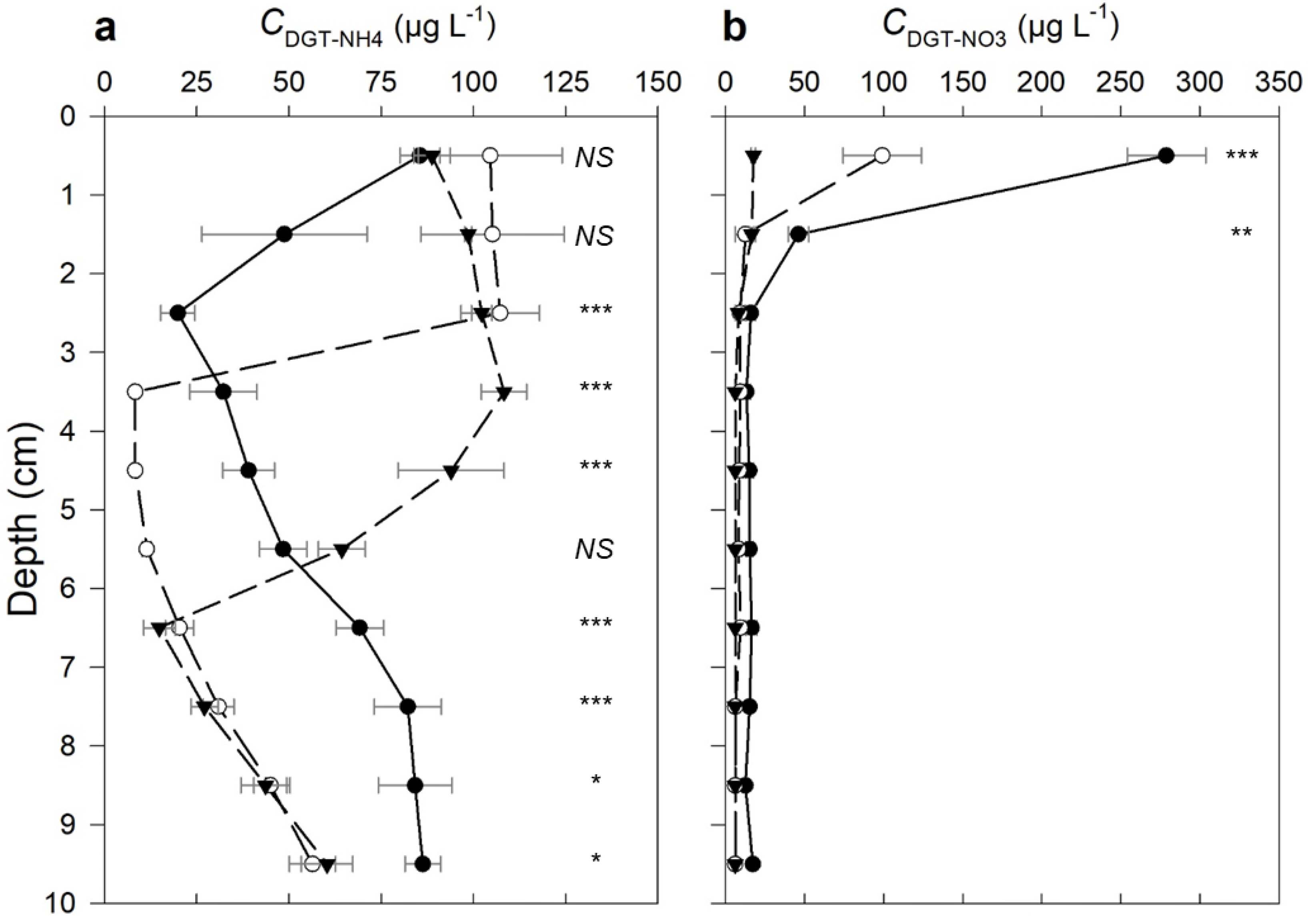
The mean CDGT-NH4 concentrations were generally highest (85.5–104.6 µg L−1) in the top 1 cm of the sediment and without significant differences between treatments (Figure 4a). The CDGT-NH4 decreased with depth to 19.9 µg L−1 by 3 cm below the SWI, while in the T5 and T20 treatments, CDGT-NH4 remained relatively constant down to 3 and 5 cm below the SWI, respectively, and then rapidly decreased to their respective minima by 4 and 7 cm below the SWI. Below these minima, the CDGT-NH4 then increased linearly with depth, where the concentration was significantly higher in the Tc sediment than in the other two sediments. The R-index in the Tc treatment ranged between 0.03 and 0.04 across the depth profile, which suggests the net consumption of NH4+ in the Tc sediments.
The highest CDGT-NO3 concentrations were observed immediately below the SWI in the Tc sediment (278 µg L−1), and concentrations in T5 and T20 were significantly lower (Figure 4b). Although NO3-N porewater concentrations (CDET-NO3) were below the MDL, it is possible to estimate minimum R-values of 0.3 and 0.1 for NO3-N in the top 1 cm of the Tc and T5 treatments, respectively; the remaining minimum R-values are <0.02. Given the low affinity of NO3− for binding to solid phases [47], the higher R-value here implies that NO3− was being generated in the top 1 cm of the Tc treatment, with net removal elsewhere.
The mean N2O fluxes over the three consecutive 24 h periods were lowest in the Tc treatment (75.61 ± 1.00 µg m−2 h−1). The gas fluxes from the mesocosms with Cu-spiked sediment were significantly higher than from the unspiked control with 110.41 ± 2.77 µg m−2 h−1 and 115.89± 1.58 µg m−2 h−1 released in the T5 and T20 mesocosms, respectively (p < 0.01); however, the difference between T5 and T20 was not significant. The addition of Cu to the two treatments resulted in N2O emissions increasing by more than 34.6 standard deviations compared to the control, Tc (effect size calculated using Glass’s d).
4. Discussion
4.1. Cycling of Nitrogen Species under Increasing Copper Concentrations
Low concentrations of Cu (8 mg kg−1) have been shown to inhibit denitrification and N2O emissions directly through acute toxic effects on denitrifying microorganisms in the short term (<1 week) [48]. However, longer-term trials have shown that the denitrifying microbial community can adapt to the increased Cu pressure within the time scale of the experiments discussed here [49,50]. Increasing Cu bioavailability has been more commonly associated with increasing nitrous oxide reductase gene expression and enzyme synthesis, thus promoting reduction of N2O to dinitrogen gas N2 [51,52,53]; however, the results from this study suggest that Cu can also affect other aspects of N cycling in sediments both directly and indirectly.
The relatively high CDGT-NH4 concentrations immediately below the SWI in all treatments are most likely driven by a combination of fast aerobic mineralisation of the sediment organic matter, partly supported by diffusion from the overlying flow of oxygenated river water, and biological nitrogen fixation [54]. The overall depletion of NH4+ (c.f. R < 0.04) is the result of the oxidation of NH4+ to nitrite (NO2−), and then NO3− (i.e., nitrification), which resupplies NO3-N in the Tc sediment together with diffusion of NO3− from the moving water above the SWI (c.f. R > 0.3). The Cu applied to the T5 and T20 sediments is likely to have at least partly disrupted the former process, as evidenced by the reduced NO3− mobilisation near the SWI (Figure 4b) and a change in the extent to which NH4+ is retained in T5 and T20 (Figure 4a).
The lower rate of NO3− production in the top 1 cm of sediment and increased N2O fluxes in T5 and T20 may be due to one or a combination of multiple factors. Firstly, NO3− generation through nitrification may have been inhibited. Wang et al. [55] showed that ammonia monooxygenase enzyme activity in river sediments decreased by ca. 25% and 59% under Cu concentrations of 50 and 100 mg kg−1, respectively, after 60 days of incubation, with similar changes in amoA gene abundance (ca. 23% and 53%, respectively). Secondly, NO3− in the Cu-treated sediments may have been reduced by the abundant ferrous iron, Fe(II); in these sediments, this can be catalysed by enzymes [56] and Cu2+ and iron (oxhydr)oxides [57,58]. Nitrate generation can also have been impacted indirectly by other processes that removed NO2−: the critical intermediate species through which numerous processes in N cycling, including nitrification, proceed. Biologically driven reduction of NO2− to nitric oxide (NO) is usually associated with Cu2+ and Cu+ through their complexes within the nitrite reductase enzyme [59]. However, the abundant Fe(II) in the treated sediments may have also facilitated the further abiotic reduction of NO2− through chemodenitrification. This process has previously been observed in circumneutral pH sediments and associated with an increased N2O:N2 ratio in gaseous N release [60,61,62,63]. Furthermore, laboratory tests have shown that some ligand–Cu complexes can catalyse the abiotic reduction of NO2− under environmentally relevant conditions [64]. One group of such Cu–ligand complexes that are most obviously relevant to aquatic environments is Cu complexed by phenolic ligands [65], which are ubiquitous in organic matter [66]: the major binding phase for Cu in these sediments (Figure S1). However, this mode of chemodenitrification, which is conceivably relevant to Cu-enriched environments, has not yet been reported outside of carefully controlled laboratory conditions using synthetic ligands.
Sustained NH4+ concentrations in the top 3 and 5 cm of the T5 and T20 sediments, respectively (Figure 4a), may be partly due to the aforementioned toxic effects of Cu on nitrifying microorganisms and partly through increased dissimilatory nitrate reduction to ammonium (DNRA). Generation of NH4+ by DNRA also consumes NO2− [67] and could further explain the reduced rate of NO3− formation in T5 and T20. The low availability of NO3− and high concentrations of Fe(II) have been linked to increased DNRA activity [68,69]. These factors may explain why relatively high CDGT-NH4 concentrations persist to greater depths in T5 and T20 and also why they subsequently decrease with depth. They also suggest that most of the N2O in the Cu-treated sediments is generated near the SWI, where nitrification rates would be expected to generate high concentrations of NO2−, while a net removal of NO2− deeper in the sediment would also reduce N2O formation.
Although dissolved oxygen profiles were not measured in this work, oxygen limitation below 2 cm may be surmised from the low CDGT-NO3 and generally increasing dissolved Fe concentrations with depth (Figure 2b and Figure 3b). Anaerobic NH4+ oxidation by NO2− (anammox), iron (oxyhydr)oxide minerals (feammox) and sulphate (sulfammox) can deplete NH4+ under anoxic conditions, and, all other things being equal, the energy yield from these processes decreases in the stated order [10]. The inhibition of anammox by Cu is well-recognised in wastewater systems [70,71]. While similar effects have not yet been shown in sediments, this could explain why the gradual depletion of CDGT-NH4 with depth in the Tc sediment between depths of 1–3 cm is not mirrored in T5 and T20. Below 3 cm, the depletion of CDGT-NH4 in T5 and T20 may be explained by the other forms of NH4+ oxidation. Feammox is thought to be driven mainly through two types of reactions, with either N2 or NO2− as the end product (e.g., Equations (3) and (4) [10]), and is believed to be less sensitive to Cu [72,73].
NH4+ + 3FeOOH + 5H+ → 0.5 N2 + 3Fe2+ + 9H2O
NH4+ + 6FeOOH + 10H+ → NO2− + 6Fe2+ + 10H2O
The consumption of H+ ions in the dissimilatory reductive dissolution of Fe(III) minerals to Fe(II) [74] and feammox would be expected to promote the sorption of Cu to solid phases [75] and thus explain the low CDGT-Cu concentrations at depths between 3 and 7 cm in the treated sediments. Direct oxidation of ammonium to N2 (Equation (3)) is thought to be the only thermodynamically viable process under the circumneutral pH found in the sediments discussed here [10,73]; however, evidence from scientific literature does not fully support this. Yao et al. [76] identified the direct oxidation of NH4+ to N2 (Equation (3)) in the presence of Fe(III) as the predominant process in slightly alkaline lake sediments (pH 7.1–7.6). On the other hand, Huang et al. [77] reported NH4+ oxidation and Fe(III) reduction at pH 6.2, albeit at a reduced rate than at lower pHs, which they attributed to the latter process (Equation (4)). Feammox to NO2− is the only process below 3 cm in the treated sediments that could conceivably generate substrate for N2O production, but the balance of evidence above suggests that it was less important in the sediment discussed here.
The oxidation of NH4+ to N2 by sulfate (sulfammox; Equation (5)) is a relatively recent discovery [78].
8NH4+ + 3SO42− → 4N2 + 3HS2− + 12H2O + 5H+
Incubation studies on marine sediments have suggested that sulfammox may act as a barrier to upward diffusive fluxes of NH4+ in sediments [79,80]. The relatively low energy yield from the process means that its role in NH4+ oxidation is likely to be most important when the energy yield from anammox and feammox has decreased due to progressively greater inhibition by the Cu in T5 and then T20 and lack of substrate: NO2− and labile iron (oxyhydr)oxide phases at depth. The increasing role of sulfammox in NH4+ removal may be the reason for the concomitant decreases in CDGT-Fe, CDGT-Mn and CDGT-NH4 and the increase in CDGT-Cu between 4 and 8 cm below the SWI in the T20 treatments. The sulfide (S2−) that is produced in this process is well-known to remove Fe(II) from the solution by forming pyrite (FeS2), which can, in turn, sequester Mn [81]. Moreover, while the formation of CuS minerals with sulfide in sediments is not well understood, the combination of reduction of Cu2+ to Cu+ by S2− and H+ ion release could conceivably mobilise Cu from the organic matter fraction.
4.2. Iron and Manganese Mobilisation in the Mesocosms
As noted above, increased Fe mobilisation in T5 and T20 sediments is likely to have played a key role in the cycling of N in these sediments. There is some suggestion that manganese can also play a key role in the redox reactions that govern N speciation [10]; however, most research to date has focussed on Fe. In addition to the dissimilatory reduction of iron (oxyhydr)oxide solid phases and mobilisation of Fe(II) by feammox in the deeper layers of the sediments, the desorption of both Fe and Mn through increased cation exchange from solid-phase binding sites is also likely to have been important throughout the depth profiles. The DGT samples solute through a controlled perturbation of the sediment, which results in diffusion of solutes from porewater into the probe and subsequent desorption from labile solid phases, while extraction using relatively strong salt solutions (1 M MgCl2 here) releases sorbed solute via cation exchange [45]. It follows that the latter is likely to provide a measure of a large pool of Fe that can be desorbed and, accordingly, was not as significantly affected by the Cu treatment here (Figure 3b). The CDGT-Fe measurement, which measures mostly Fe(II) due to the low solubility of Fe(III) at circumneutral pH, is more sensitive to differences in porewater concentrations and thus more likely to be representative of the chemically labile and bioavailable Fe. On the other hand, exchangeable Mn concentrations appeared to be affected by the Cu treatment (Figure 3c) and generally mirror the CDGT-Mn measurements (Figure 2c), which suggests that the sorbed pool of Mn(II) is relatively small and labile. The depletion of NO3− in T5 and T20 may also have resulted in some reductive dissolution of Mn near the SWI, thus increasing the solubility of the metal.
4.3. Mesocosm Experiments
The experimental approach used here was chosen to establish a system that could be replicated and carefully controlled to test the effect of Cu contamination systematically. However, this approach has numerous limitations that should be recognised. The extensive disturbance of the sediment during sampling and processing before the start of the equilibration is likely to have disrupted many of the natural microbiological processes and redox gradients in the sediment. Others have found that equilibration periods of three weeks are sufficient for helping to restore steady-state gradients in sediments [82]; this is confirmed by the extended equilibration period used in this study, while monitoring the water quality variables and N species concentrations in the circulating water.
The rates of N2O production measured in this study were slightly above the ranges measured elsewhere. For example, Clough and Kelliher [83] reported fluxes of 3–87 µg m−2 h−1 in situ above the sediments of the Waikato River in New Zealand. This is probably because the water flow was turned off for the duration of the N2O measurements. This was an experimental necessity but would have reduced the diffusive flux of oxygen into the sediment and increased rates of denitrification in the sediment columns. While this is unlikely to have affected the main aim of the experiment, the absolute fluxes should be considered more representative of quiescent water courses in an agricultural landscape than rivers. Such watercourses can include ponds and drains that have ephemeral flows during the summer months and can also reach higher temperatures than perennially flowing systems [84].
Depth profile measurements using high-resolution DGT, where the mass of bound solute is analysed through a technique that can achieve extremely high spatial resolution (e.g., <10 µm resolution using LA-ICP-MS or colorimetry), have revealed unique details about diagenetic processes in sediments [85]. Such methods require very thin diffusion layers between the resin gel and the sediment to minimise lateral diffusion within the diffusion layer and loss of spatial resolution [86]. The trade-off from using very thin diffusion layers is the strong depletion of the solute concentration at the probe interface. Consequently, the calculated CDGT concentrations rarely represent the local solute concentration in the bulk sediment, and the results are often reported and discussed as fluxes rather than concentrations. In this study, a coarser spatial resolution was seen appropriate to achieve the objectives of this research. Although some fine details on elemental cycling at specific parts of the sediment depth profile were undoubtedly lost, what was gained in return was the ability to compare between replicates and quantitatively analyse how Cu affects the dynamics of N-species at different depths in the sediment. The thicker diffusion layer also allowed for general estimates of R-values to indicate where production or loss of solute was occurring, which is particularly useful when considering highly dynamic species such as NO3− and NH4+, whose concentrations are likely to change during the typical 24 h DGT deployment.
5. Conclusions
The ANZECC guideline values of 65 and 270 mg kg−1 for Cu in sediments seek to minimise potential harm posed by the metal and protect local ecosystems. However, our results show that lower Cu concentrations can have previously unrecognised implications for nitrogen biogeochemistry in freshwater sediments and greenhouse gas emissions arising from Cu contamination in New Zealand. The replicated mesocosm approach used here has served to demonstrate the potential for such effects under well-controlled, quiescent and flowing water conditions. The next step should now be to further validate these discoveries in the field.
Supplementary Materials
The following supporting information can be downloaded at: https://www.mdpi.com/article/10.3390/su15139958/s1.
Author Contributions
T.T. executed all experimental work and data analysis and helped to conceive the experimental design and draft an early version of the manuscript. J.H. contributed her expertise in the manufacture and use of DGT probes for measuring NO3− and NH4+ and reviewed the manuscript. N.J.L. helped to conceive the experimental design and oversaw all aspects of the research, including preparing the final draft of the manuscript. All authors have read and agreed to the published version of the manuscript.
Funding
This research received no external funding.
Institutional Review Board Statement
Not applicable.
Informed Consent Statement
Not applicable.
Data Availability Statement
The data presented in this study are available on request from the corresponding author.
Acknowledgments
The senior author would like to thank NZAID for a master’s scholarship. We are also grateful to T. J. Clough (Lincoln University) for his feedback on an early experimental design and advice on measuring N2O gas fluxes.
Conflicts of Interest
The authors declare no conflict of interest.
References
- Meybeck, M. Global analysis of river systems: From Earth system controls to Anthropocene syndromes. Philos. Trans. R. Soc. B Biol. Sci. 2003, 358, 1935–1955. [Google Scholar] [CrossRef] [PubMed] [Green Version]
- Miralles-Wilhelm, F.; Matthews, J.H.; Karres, N.; Abell, R.; Dalton, J.; Kang, S.-T.; Liu, J.; Maendly, R.; Matthews, N.; McDonald, R.; et al. Emerging themes and future directions in watershed resilience research. Water Secur. 2023, 18, 100132. [Google Scholar] [CrossRef]
- Gaillardet, J.; Viers, J.; Dupré, B. Trace Elements in River Waters. In Treatise on Geochemistry; Holland, H.D., Turekian, K.K., Eds.; Elsevier Ltd.: Amsterdam, The Netherlands, 2003; Volume 5, pp. 225–272. [Google Scholar] [CrossRef]
- Zhao, J.; Wu, E.; Zhang, B.; Bai, X.; Lei, P.; Qiao, X.; Li, Y.-F.; Li, B.; Wu, G.; Gao, Y. Pollution characteristics and ecological risks associated with heavy metals in the Fuyang river system in North China. Environ. Pollut. 2021, 281, 116994. [Google Scholar] [CrossRef] [PubMed]
- Nystrand, M.I.; Österholm, P.; Nyberg, M.E.; Gustafsson, J.P. Metal speciation in rivers affected by enhanced soil erosion and acidity. Appl. Geochem. 2012, 27, 906–916. [Google Scholar] [CrossRef]
- Loureiro, R.C.; Calisto, J.F.F.; Magro, J.D.; Restello, R.M.; Hepp, L.U. The influence of the environment in the incorporation of copper and cadmium in scraper insects. Environ. Monit. Assess. 2021, 193, 215. [Google Scholar] [CrossRef]
- Marschner, H. Marschner’s Mineral Nutrition of Higher Plants; Academic Press: Cambridge, MA, USA, 2011. [Google Scholar]
- Erisman, J.W.; Sutton, M.A.; Galloway, J.; Klimont, Z.; Winiwarter, W. How a century of ammonia synthesis changed the world. Nat. Geosci. 2008, 1, 636–639. [Google Scholar] [CrossRef]
- Galloway, J.N.; Aber, J.D.; Erisman, J.W.; Seitzinger, S.P.; Howarth, R.W.; Cowling, E.B.; Cosby, B.J. The Nitrogen Cascade. BioScience 2003, 53, 341–356. [Google Scholar] [CrossRef]
- Thamdrup, B. New Pathways and Processes in the Global Nitrogen Cycle. Annu. Rev. Ecol. Evol. Syst. 2012, 43, 407–428. [Google Scholar] [CrossRef]
- Quick, A.M.; Reeder, W.J.; Farrell, T.B.; Tonina, D.; Feris, K.P.; Benner, S.G. Nitrous oxide from streams and rivers: A review of primary biogeochemical pathways and environmental variables. Earth-Sci. Rev. 2019, 191, 224–262. [Google Scholar] [CrossRef]
- Roberto, A.A.; Van Gray, J.B.; Leff, L.G. Sediment bacteria in an urban stream: Spatiotemporal patterns in community composition. Water Res. 2018, 134, 353–369. [Google Scholar] [CrossRef]
- Seeley, M.E.; Song, B.; Passie, R.; Hale, R.C. Microplastics affect sedimentary microbial communities and nitrogen cycling. Nat. Commun. 2020, 11, 2372. [Google Scholar] [CrossRef]
- Rother, J.A.; Millbank, J.W.; Thornton, I. Effects of heavy-metal additions on ammonification and nitrification in soils contaminated with cadmium, lead and zinc. Plant Soil 1982, 69, 239–258. [Google Scholar] [CrossRef]
- Li, C.; Quan, Q.; Gan, Y.; Dong, J.; Fang, J.; Wang, L.; Liu, J. Effects of heavy metals on microbial communities in sediments and establishment of bioindicators based on microbial taxa and function for environmental monitoring and management. Sci. Total. Environ. 2020, 749, 141555. [Google Scholar] [CrossRef]
- Babich, H.; Stotzky, G. Heavy metal toxicity to microbe-mediated ecologic processes: A review and potential application to regulatory policies. Environ. Res. 1985, 36, 111–137. [Google Scholar] [CrossRef]
- Hoostal, M.J.; Bidart-Bouzat, M.G.; Bouzat, J.L. Local adaptation of microbial communities to heavy metal stress in polluted sediments of Lake Erie. FEMS Microbiol. Ecol. 2008, 65, 156–168. [Google Scholar] [CrossRef] [Green Version]
- Flemming, C.A.; Trevors, J.T. Copper toxicity and chemistry in the environment: A review. Water Air Soil Pollut. 1989, 44, 143–158. [Google Scholar] [CrossRef]
- Lushchak, V.I. Environmentally induced oxidative stress in aquatic animals. Aquat. Toxicol. 2011, 101, 13–30. [Google Scholar] [CrossRef]
- He, Z.L.; Yang, X.E.; Stoffella, P.J. Trace elements in agroecosystems and impacts on the environment. J. Trace Elem. Med. Biol. 2005, 19, 125–140. [Google Scholar] [CrossRef]
- Morgan, R.K.; Taylor, E. Copper Accumulation in Vineyard Soils in New Zealand. Environ. Sci. 2004, 1, 139–167. [Google Scholar] [CrossRef] [Green Version]
- Bolan, N.S.; Khan, M.A.; Donaldson, J.; Adriano, D.C.; Matthew, C. Distribution and bioavailability of copper in farm effluent. Sci. Total Environ. 2003, 309, 225–236. [Google Scholar] [CrossRef]
- Fernández, D.; Voss, K.; Bundschuh, M.; Zubrod, J.P.; Schäfer, R.B. Effects of fungicides on decomposer communities and litter decomposition in vineyard streams. Sci. Total. Environ. 2015, 533, 40–48. [Google Scholar] [CrossRef] [PubMed]
- Bereswill, R.; Golla, B.; Streloke, M.; Schulz, R. Entry and toxicity of organic pesticides and copper in vineyard streams: Erosion rills jeopardise the efficiency of riparian buffer strips. Agric. Ecosyst. Environ. 2012, 146, 81–92. [Google Scholar] [CrossRef]
- Pennington, S.L.; Webster-Brown, J.G. Stormwater runoff quality from copper roofing, Auckland, New Zealand. N. Z. J. Marit. Freshw. Res. 2008, 42, 99–108. [Google Scholar] [CrossRef] [Green Version]
- ANZECC/ARMCANZ. Australian and New Zealand Guidelines for Fresh and Marine Water Quality; Australian and New Zealand Environment and Conservation Council and Agriculture and Resource Management Council of Australia and New Zealand: Canberra, Australia, 2000; Volume 1, pp. 1–314. [Google Scholar]
- Ahlf, W.; Drost, W.; Heise, S. Incorporation of metal bioavailability into regulatory frameworks—Metal exposure in water and sediment. J. Soils Sediments 2009, 9, 411–419. [Google Scholar] [CrossRef]
- Magalhães, C.; Costa, J.; Teixeira, C.; Bordalo, A.A. Impact of trace metals on denitrification in estuarine sediments of the Douro River estuary, Portugal. Mar. Chem. 2007, 107, 332–341. [Google Scholar] [CrossRef]
- Sakadevan, K.; Zheng, H.; Bavor, H. Impact of heavy metals on denitrification in surface wetland sediments receiving wastewater. Water Sci. Technol. 1999, 40, 349–355. [Google Scholar] [CrossRef]
- Vázquez-Blanco, R.; Arias-Estévez, M.; Bååth, E.; Fernández-Calviño, D. Comparison of Cu salts and commercial Cu based fungicides on toxicity towards microorganisms in soil. Environ. Pollut. 2019, 257, 113585. [Google Scholar] [CrossRef]
- Sutcliffe, B.; Hose, G.; Harford, A.; Midgley, D.; Greenfield, P.; Paulsen, I.; Chariton, A. Microbial communities are sensitive indicators for freshwater sediment copper contamination. Environ. Pollut. 2019, 247, 1028–1038. [Google Scholar] [CrossRef]
- Froelich, P.; Klinkhammer, G.; Bender, M.; Luedtke, N.; Heath, G.; Cullen, D.; Dauphin, P.; Hammond, D.; Hartman, B.; Maynard, V. Early oxidation of organic matter in pelagic sediments of the eastern equatorial Atlantic—Suboxic diagenesis. Geochim. Cosmochim. Acta 1979, 43, 1075–1090. [Google Scholar] [CrossRef]
- Chen, J.; Erler, D.V.; Wells, N.S.; Huang, J.; Welsh, D.T.; Eyre, B.D. Denitrification, anammox, and dissimilatory nitrate reduction to ammonium across a mosaic of estuarine benthic habitats. Limnol. Oceanogr. 2021, 66, 1281–1297. [Google Scholar] [CrossRef]
- Morgan, T.K.K.B. Waiora and Cultural Identity: Water quality assessment using the Mauri Model. Altern. Int. J. Indig. Peoples 2006, 3, 42–67. [Google Scholar] [CrossRef]
- Land, Air, Water, Aotearoa (LAWA) (n.d.). LII Stream at Pannetts Road Bridge. Available online: https://www.lawa.org.nz/explore-data/canterbury-region/river-quality/ellesmere-waihora-catchment/lii-stream-at-pannetts-road-bridge/ (accessed on 25 March 2021).
- Simmler, M.; Ciadamidaro, L.; Schulin, R.; Madejón, P.; Reiser, R.; Clucas, L.; Weber, P.; Robinson, B. Lignite Reduces the Solubility and Plant Uptake of Cadmium in Pasturelands. Environ. Sci. Technol. 2013, 47, 4497–4504. [Google Scholar] [CrossRef]
- Clough, T.J.; Addy, K.; Kellogg, D.Q.; Nowicki, B.L.; Gold, A.J.; Groffman, P.M. Dynamics of nitrous oxide in groundwater at the aquatic-terrestrial interface. Glob. Chang. Biol. 2007, 13, 1528–1537. [Google Scholar] [CrossRef]
- Clough, T.; Kelliher, F.; Wang, Y.; Sherlock, R. Diffusion of 15N-labelled N2O into soil columns: A promising method to examine the fate of N2O in subsoils. Soil Biol. Biochem. 2006, 38, 1462–1468. [Google Scholar] [CrossRef]
- Zhang, H.; Davison, W.; Miller, S.; Tych, W. In situ high resolution measurements of fluxes of Ni, Cu, Fe, and Mn and concentrations of Zn and Cd in porewaters by DGT. Geochim. Cosmochim. Acta 1995, 59, 4181–4192. [Google Scholar] [CrossRef]
- Huang, J.; Franklin, H.; Teasdale, P.R.; Burford, M.A.; Kankanamge, N.R.; Bennett, W.W.; Welsh, D.T. Comparison of DET, DGT and conventional porewater extractions for determining nutrient profiles and cycling in stream sediments. Environ. Sci. Process. Impacts 2019, 21, 2128–2140. [Google Scholar] [CrossRef]
- Jolley, D.F.; Mason, S.; Gao, Y.; Zhang, H. Practicalities of working with DGT. Diffusive Gradients in Thin Films for Environmental Measurements. In Diffusive Gradients in Thin-Films for Environmental Measurements; Davison, W., Ed.; Cambridge University Press: Cambridge, UK, 2016; pp. 263–290. [Google Scholar]
- Huang, J.; Bennett, W.W.; Welsh, D.T.; Li, T.; Teasdale, P.R. Development and evaluation of a diffusive gradients in a thin film technique for measuring ammonium in freshwaters. Anal. Chim. Acta 2016, 904, 83–91. [Google Scholar] [CrossRef]
- Huang, J.; Bennett, W.W.; Teasdale, P.R.; Kankanamge, N.R.; Welsh, D.T. A modified DGT technique for the simultaneous measurement of dissolved inorganic nitrogen and phosphorus in freshwaters. Anal. Chim. Acta 2017, 988, 17–26. [Google Scholar] [CrossRef]
- Garmo, A.; Røyset, O.; Steinnes, E.; Flaten, T.P. Performance Study of Diffusive Gradients in Thin Films for 55 Elements. Anal. Chem. 2003, 75, 3573–3580. [Google Scholar] [CrossRef]
- Lehto, N.J. Principles and Application in Soils and Sediments. In Diffusive Gradients in Thin-Films for Environmental Measurements; Davison, W., Ed.; Cambridge University Press: Cambridge, UK, 2016; pp. 146–173. [Google Scholar]
- Tessier, A.; Campbell, P.G.C.; Bisson, M. Sequential extraction procedure for the speciation of particulate trace metals. Anal. Chem. 1979, 51, 844–851. [Google Scholar] [CrossRef]
- Hantush, M.M. Modeling nitrogen-carbon cycling and oxygen consumption in bottom sediments. Adv. Water Resour. 2007, 30, 59–79. [Google Scholar] [CrossRef]
- Magalhães, C.M.; Machado, A.; Matos, P.; Bordalo, A.A. Impact of copper on the diversity, abundance and transcription of nitrite and nitrous oxide reductase genes in an urban European estuary. FEMS Microbiol. Ecol. 2011, 77, 274–284. [Google Scholar] [CrossRef] [PubMed] [Green Version]
- Holtan-Hartwig, L.; Bechmann, M.; Høyås, T.R.; Linjordet, R.; Bakken, L.R. Heavy metals tolerance of soil denitrifying communities: N2O dynamics. Soil Biol. Biochem. 2002, 34, 1181–1190. [Google Scholar] [CrossRef]
- Guo, Q.; Li, N.; Bing, Y.; Chen, S.; Zhang, Z.; Chang, S.; Chen, Y.; Xie, S. Denitrifier communities impacted by heavy metal contamination in freshwater sediment. Environ. Pollut. 2018, 242, 426–432. [Google Scholar] [CrossRef]
- Felgate, H.; Giannopoulos, G.; Sullivan, M.J.; Gates, A.J.; Clarke, T.A.; Baggs, E.; Rowley, G.; Richardson, D.J. The impact of copper, nitrate and carbon status on the emission of nitrous oxide by two species of bacteria with biochemically distinct denitrification pathways. Environ. Microbiol. 2012, 14, 1788–1800. [Google Scholar] [CrossRef]
- Sullivan, M.J.; Gates, A.J.; Appia-Ayme, C.; Rowley, G.; Richardson, D.J. Copper control of bacterial nitrous oxide emission and its impact on vitamin B12-dependent metabolism. Proc. Natl. Acad. Sci. USA 2013, 110, 19926–19931. [Google Scholar] [CrossRef] [Green Version]
- Giannopoulos, G.; Hartop, K.R.; Brown, B.L.; Song, B.; Elsgaard, L.; Franklin, R.B. Trace Metal Availability Affects Greenhouse Gas Emissions and Microbial Functional Group Abundance in Freshwater Wetland Sediments. Front. Microbiol. 2020, 11, 560861. [Google Scholar] [CrossRef]
- Bakker, E.A.H.; Vizza, C.; Arango, C.P.; Roley, S.S. Nitrogen fixation rates in forested mountain streams: Are sediment microbes more important than previously thought? Freshw. Biol. 2022, 67, 1395–1410. [Google Scholar] [CrossRef]
- Wang, L.; Li, Y.; Niu, L.; Zhang, W.; Zhang, H.; Wang, L.; Wang, P. Response of ammonia oxidizing archaea and bacteria to decabromodiphenyl ether and copper contamination in river sediments. Chemosphere 2018, 191, 858–867. [Google Scholar] [CrossRef]
- Schaedler, F.; Lockwood, C.; Lueder, U.; Glombitza, C.; Kappler, A.; Schmidt, C. Microbially Mediated Coupling of Fe and N Cycles by Nitrate-Reducing Fe(II)-Oxidizing Bacteria in Littoral Freshwater Sediments. Appl. Environ. Microbiol. 2018, 84, e02013-17. [Google Scholar] [CrossRef] [Green Version]
- Ottley, C.; Davison, W.; Edmunds, W. Chemical catalysis of nitrate reduction by iron (II). Geochim. Cosmochim. Acta 1997, 61, 1819–1828. [Google Scholar] [CrossRef]
- Picardal, F. Abiotic and microbial interactions during anaerobic transformations of Fe (II) and NOx. Front. Microbiol. 2012, 3, 112. [Google Scholar] [CrossRef] [Green Version]
- Kuypers, M.M.M.; Marchant, H.K.; Kartal, B. The microbial nitrogen-cycling network. Nat. Rev. Microbiol. 2018, 16, 263–276. [Google Scholar] [CrossRef]
- Tai, Y.-L.; Dempsey, B.A. Nitrite reduction with hydrous ferric oxide and Fe(II): Stoichiometry, rate, and mechanism. Water Res. 2009, 43, 546–552. [Google Scholar] [CrossRef]
- Li, X.; Sardans, J.; Hou, L.; Gao, D.; Liu, M.; Peñuelas, J. Dissimilatory Nitrate/Nitrite Reduction Processes in River Sediments Across Climatic Gradient: Influences of Biogeochemical Controls and Climatic Temperature Regime. J. Geophys. Res. Biogeosciences 2019, 124, 2305–2320. [Google Scholar] [CrossRef] [Green Version]
- Chen, D.; Yuan, X.; Zhao, W.; Luo, X.; Li, F.; Liu, T. Chemodenitrification by Fe(II) and nitrite: pH effect, mineralization and kinetic modeling. Chem. Geol. 2020, 541, 119586. [Google Scholar] [CrossRef]
- Jones, L.C.; Peters, B.; Pacheco, J.S.L.; Casciotti, K.L.; Fendorf, S. Stable Isotopes and Iron Oxide Mineral Products as Markers of Chemodenitrification. Environ. Sci. Technol. 2015, 49, 3444–3452. [Google Scholar] [CrossRef]
- Woollard-Shore, J.G.; Holland, J.P.; Jones, M.W.; Dilworth, J.R. Nitrite reduction by copper complexes. Dalton Trans. 2010, 39, 1576–1585. [Google Scholar] [CrossRef]
- Mondal, A.; Reddy, K.P.; Bertke, J.A.; Kundu, S. Phenol Reduces Nitrite to NO at Copper(II): Role of a Proton-Responsive Outer Coordination Sphere in Phenol Oxidation. J. Am. Chem. Soc. 2020, 142, 1726–1730. [Google Scholar] [CrossRef]
- Tipping, E.; Lofts, S.; Sonke, J. Humic Ion-Binding Model VII: A revised parameterisation of cation-binding by humic substances. Environ. Chem. 2011, 8, 225–235. [Google Scholar] [CrossRef] [Green Version]
- Burgin, A.J.; Hamilton, S.K. Have we overemphasized the role of denitrification in aquatic ecosystems? A review of nitrate removal pathways. Front. Ecol. Environ. 2007, 5, 89–96. [Google Scholar] [CrossRef] [Green Version]
- Dong, L.F.; Smith, C.J.; Papaspyrou, S.; Stott, A.; Osborn, A.M.; Nedwell, D.B. Changes in Benthic Denitrification, Nitrate Ammonification, and Anammox Process Rates and Nitrate and Nitrite Reductase Gene Abundances along an Estuarine Nutrient Gradient (the Colne Estuary, United Kingdom). Appl. Environ. Microbiol. 2009, 75, 3171–3179. [Google Scholar] [CrossRef] [PubMed] [Green Version]
- Robertson, E.K.; Thamdrup, B. The fate of nitrogen is linked to iron(II) availability in a freshwater lake sediment. Geochim. Et Cosmochim. Acta 2017, 205, 84–99. [Google Scholar] [CrossRef] [Green Version]
- Zhang, Q.-Q.; Yang, G.-F.; Wang, H.; Wu, K.; Jin, R.-C.; Zheng, P. Estimating the recovery of ANAMMOX performance from inhibition by copper (II) and oxytetracycline (OTC). Sep. Purif. Technol. 2013, 113, 90–103. [Google Scholar] [CrossRef]
- Mak, C.; Lin, J.; Bashir, M. An overview of the effects of heavy metals content in wastewater on anammox bacteria. Adv. Environ. Stud. 2018, 2, 61–70. [Google Scholar]
- Zhang, Z.-Z.; Deng, R.; Cheng, Y.-F.; Zhou, Y.-H.; Buayi, X.; Zhang, X.; Wang, H.-Z.; Jin, R.-C. Behavior and fate of copper ions in an anammox granular sludge reactor and strategies for remediation. J. Hazard. Mater. 2015, 300, 838–846. [Google Scholar] [CrossRef]
- Wan, L.; Liu, H.; Wang, X. Anaerobic ammonium oxidation coupled to Fe(III) reduction: Discovery, mechanism and application prospects in wastewater treatment. Sci. Total. Environ. 2021, 818, 151687. [Google Scholar] [CrossRef]
- Davison, W. Iron and manganese in lakes. Earth-Sci. Rev. 1993, 34, 119–163. [Google Scholar] [CrossRef]
- Stumm, W.; Morgan, J.J. Aquatic Chemistry: Chemical Equilibria and Rates in Natural Waters; John Wiley & Sons: Hoboken, NJ, USA, 2012. [Google Scholar]
- Yao, Z.; Wang, F.; Wang, C.; Xu, H.; Jiang, H. Anaerobic ammonium oxidation coupled to ferric iron reduction in the sediment of a eutrophic lake. Environ. Sci. Pollut. Res. 2019, 26, 15084–15094. [Google Scholar] [CrossRef]
- Huang, S.; Chen, C.; Peng, X.; Jaffé, P.R. Environmental factors affecting the presence of Acidimicrobiaceae and ammonium removal under iron-reducing conditions in soil environments. Soil Biol. Biochem. 2016, 98, 148–158. [Google Scholar] [CrossRef] [Green Version]
- Liu, S.; Yang, F.; Gong, Z.; Meng, F.; Chen, H.; Xue, Y.; Furukawa, K. Application of anaerobic ammonium-oxidizing consortium to achieve completely autotrophic ammonium and sulfate removal. Bioresour. Technol. 2008, 99, 6817–6825. [Google Scholar] [CrossRef]
- Rios-del Toro, E.E.; Cervantes, F.J. Coupling between anammox and autotrophic denitrification for simultaneous removal of ammonium and sulfide by enriched marine sediments. Biodegradation 2016, 27, 107–118. [Google Scholar] [CrossRef]
- Rios-del Toro, E.E.; Valenzuela, E.I.; López-Lozano, N.E.; Cortés-Martínez, M.G.; Sánchez-Rodríguez, M.A.; Calvario-Martínez, O.; Sánchez-Carrillo, S.; Cervantes, F.J. Anaerobic ammonium oxidation linked to sulfate and ferric iron reduction fuels nitrogen loss in marine sediments. Biodegradation 2018, 29, 429–442. [Google Scholar] [CrossRef]
- Morse, J.W.; Luther, G., III. Chemical influences on trace metal-sulfide interactions in anoxic sediments. Geochim. Cosmochim. Acta 1999, 63, 3373–3378. [Google Scholar] [CrossRef]
- Lehto, N.J.; Glud, R.N.; Norði, G.; Zhang, H.; Davison, W. Anoxic microniches in marine sediments induced by aggregate settlement: Biogeochemical dynamics and implications. Biogeochemistry 2014, 119, 307–327. [Google Scholar] [CrossRef]
- Clough, T.J.; Kelliher, F.M. Nitrous Oxide Emission from Waterways. New Zealand Ministry for Primary Industries Technical Paper No: 2013/05; 2013. Available online: https://www.mpi.govt.nz/dmsdocument/2960/direct (accessed on 25 March 2021).
- Woodward, K.B.; Fellows, C.S.; Conway, C.L.; Hunter, H.M. Nitrate removal, denitrification and nitrous oxide production in the riparian zone of an ephemeral stream. Soil Biol. Biochem. 2009, 41, 671–680. [Google Scholar] [CrossRef]
- Santner, J.; Williams, P.N. Measurement at High Spatial Resolution. In Diffusive Gradients in Thin-Films for Environmental Measurements; Davison, W., Ed.; Cambridge University Press: Cambridge, UK, 2016; pp. 174–215. [Google Scholar] [CrossRef]
- Lehto, N.J.; Davison, W.; Zhang, H. The use of ultra-thin diffusive gradients in thin-films (DGT) devices for the analysis of trace metal dynamics in soils and sediments: A measurement and modelling approach. Environ. Chem. 2012, 9, 415–423. [Google Scholar] [CrossRef]
Figure 1.
Sediment mesocosm with a river water circulation system (not to scale).
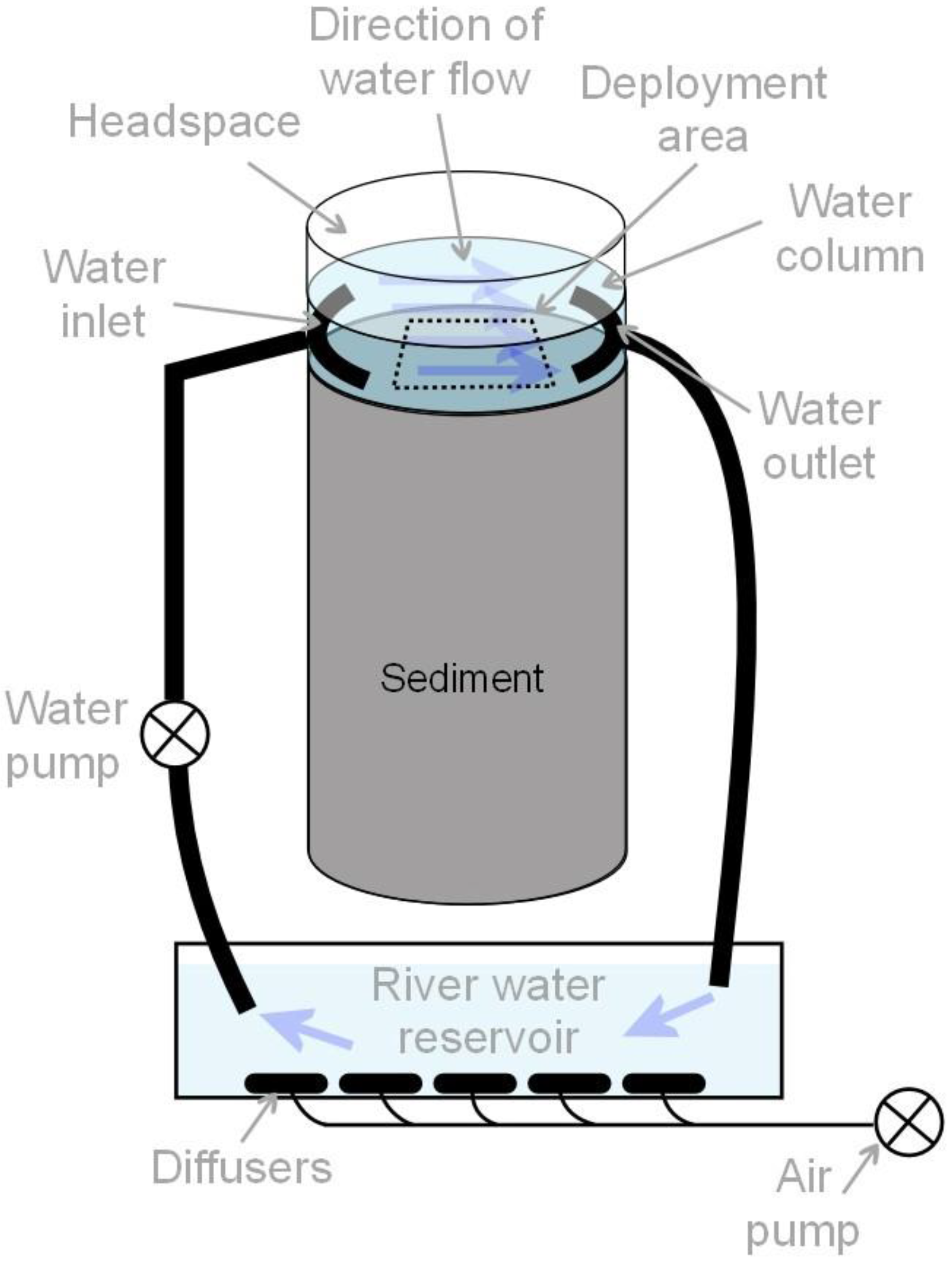
Figure 2.
DGT-measured depth profiles for (a) Cu, (b) Fe and (c) Mn at 1 cm intervals below the sediment–water interface (SWI) in the three treatments, Tc (black solid line with ●), T5 (dashed line with ○) and T20 (dashed line with ▼). The points show the average concentration across the (y-axis) depth interval ± 0.5 cm above and below the point. The error bars show standard error (n = 3). The number of asterisks indicates level of significance at each depth interval: * p < 0.05, ** p < 0.01, or *** p < 0.001; not significant is shown as NS (p > 0.05).
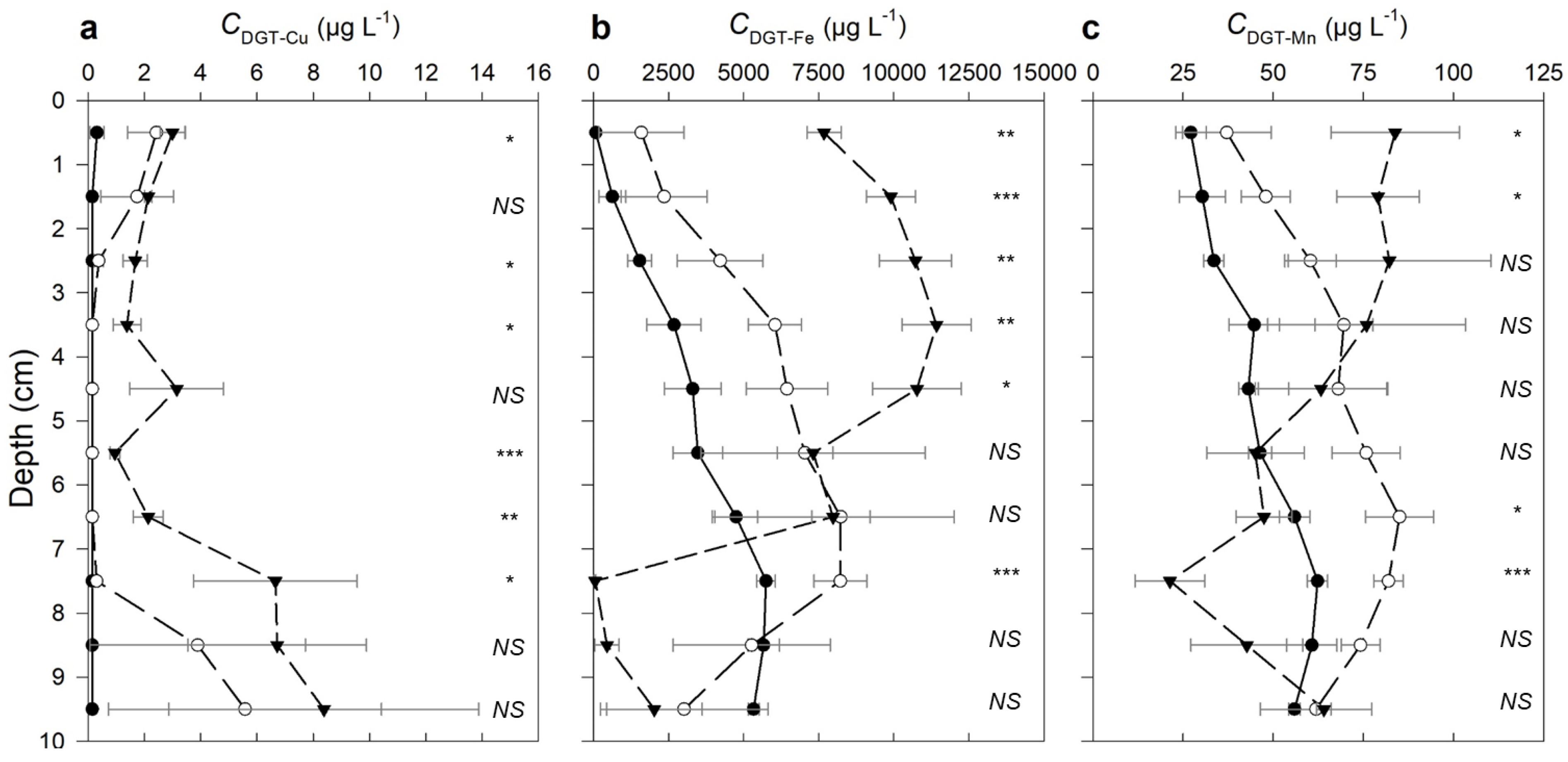
Figure 3.
Exchangeable concentrations of Cu (ExCu; a), Fe (ExFe; b) and Mn (ExMn; c) in the exchangeable fractions at 1 cm intervals below the SWI in the three treatments, Tc (black solid line with ●), T5 (dashed line with ○) and T20 (dashed line with ▼). The points show the average concentration across the (y-axis) depth interval ± 0.5 cm above and below the point. The error bars show standard error at each depth (n = 3). The number of asterisks indicates level of significance at each depth interval: * p < 0.05, ** p < 0.01, *** p < 0.001; not significant is shown as NS (p > 0.05). NB: Fe and Mn concentrations are ca. 100 and 2–3 times higher, respectively, than the highest Cu concentrations.

Figure 4.
DGT-measured depth profiles for (a) NO3-N and (b) NH4-N at 1 cm intervals below the sediment–water interface (SWI) in the three Cu treatments, Tc (black solid line with ●), T5 (dashed line with ○) and T20 (dashed line with ▼). The points show the average concentration across the (y-axis) depth interval ± 0.5 cm above and below the point. The error bars show standard error (n = 3). The number of asterisks indicates level of significance at each depth interval: * p < 0.05, ** p < 0.01, *** p < 0.001; not significant is shown as NS (p > 0.05).

Table 1.
Physical and chemical sediment characteristics. The values show averages (±standard deviation; n = 3). Different letters indicate a significant difference between treatments (p < 0.05).
Table 1.
Physical and chemical sediment characteristics. The values show averages (±standard deviation; n = 3). Different letters indicate a significant difference between treatments (p < 0.05).
| Sediment Treatment * | |||
|---|---|---|---|
| Tc | T5 | T20 | |
| Moisture (%) | 40 ± 0 | - | - |
| Organic matter (%) | 1.61 ± 0.39 | - | - |
| Total carbon (%) | 0.93 ± 0.22 | - | - |
| Total nitrogen (%) | 0.41 ± 0.01 | - | - |
| P (mg kg−1) | 475.58 ± 9.10 | - | - |
| S (mg kg−1) | 349.18 ± 26.18 | - | - |
| Exchangeable pH | 6.67 ± 0.02 a | 6.43 ± 0.13 a | 6.57 ± 0.16 a |
| Cu (mg kg−1) | 6.22 ± 0.26 c | 33.14 ± 1.35 b | 119.66 ± 1.40 a |
| Fe (mg kg−1) | 13 235 ± 345 a | 13 261 ± 41 a | 13 169 ± 85 a |
| Mn (mg kg−1) | 153.17 ± 1.28 a | 151.18 ± 0.17 a | 148 ± 3.19 a |
* Tc, T5 and T20 refer to the amount of Cu added to the sediment, where the subscript shows the factor by which the Cu concentration was increased from the original concentration in Tc. Total organic matter, C, N, P and S were only analysed in unspiked (Tc) sediment.
Disclaimer/Publisher’s Note: The statements, opinions and data contained in all publications are solely those of the individual author(s) and contributor(s) and not of MDPI and/or the editor(s). MDPI and/or the editor(s) disclaim responsibility for any injury to people or property resulting from any ideas, methods, instructions or products referred to in the content. |
© 2023 by the authors. Licensee MDPI, Basel, Switzerland. This article is an open access article distributed under the terms and conditions of the Creative Commons Attribution (CC BY) license (https://creativecommons.org/licenses/by/4.0/).
Share and Cite
MDPI and ACS Style
Tomoiye, T.; Huang, J.; Lehto, N.J. Copper Contamination Affects the Biogeochemical Cycling of Nitrogen in Freshwater Sediment Mesocosms. Sustainability 2023, 15, 9958. https://doi.org/10.3390/su15139958
AMA Style
Tomoiye T, Huang J, Lehto NJ. Copper Contamination Affects the Biogeochemical Cycling of Nitrogen in Freshwater Sediment Mesocosms. Sustainability. 2023; 15(13):9958. https://doi.org/10.3390/su15139958
Chicago/Turabian StyleTomoiye, Tomson, Jianyin Huang, and Niklas J. Lehto. 2023. "Copper Contamination Affects the Biogeochemical Cycling of Nitrogen in Freshwater Sediment Mesocosms" Sustainability 15, no. 13: 9958. https://doi.org/10.3390/su15139958
Note that from the first issue of 2016, this journal uses article numbers instead of page numbers. See further details here.