Water Level Prediction through Hybrid SARIMA and ANN Models Based on Time Series Analysis: Red Hills Reservoir Case Study

Abstract

Reservoir water level (RWL) prediction has become a challenging task due to spatio-temporal changes in climatic conditions and complicated physical process. The Red Hills Reservoir (RHR) is an important source of drinking and irrigation water supply in Thiruvallur district, Tamil Nadu, India, also expected to be converted into the other productive services in the future. However, climate change in the region is expected to have consequences over the RHR’s future prospects. As a result, accurate and reliable prediction of the RWL is crucial to develop an appropriate water release mechanism of RHR to satisfy the population’s water demand. In the current study, time series modelling technique was adopted for the RWL prediction in RHR using Box–Jenkins autoregressive seasonal autoregressive integrated moving average (SARIMA) and artificial neural network (ANN) hybrid models. In this research, the SARIMA model was obtained as SARIMA (0, 0, 1) (0, 3, 2)₁₂ but the residual of the SARIMA model could not meet the autocorrelation requirement of the modelling approach. In order to overcome this weakness of the SARIMA model, a new SARIMA–ANN hybrid time series model was developed and demonstrated in this study. The average monthly RWL data from January 2004 to November 2020 was used for developing and testing the models. Several model assessment criteria were used to evaluate the performance of each model. The findings showed that the SARIMA–ANN hybrid model outperformed the remaining models considering all performance criteria for reservoir RWL prediction. Thus, this study conclusively proves that the SARIMA–ANN hybrid model could be a viable option for the accurate prediction of reservoir water level.

1. Introduction

Each region has its own set of water quality and quantity concerns, depending on the climatic, geographic, geologic, social, and economic characteristics. The rainfall pattern is likely to shift all over the planet as a result of global warming and climate change. Modelling studies until the year 2050 have anticipated that the world’s freshwater distribution is expected to undergo a paradigm shift [1,2]. Therefore, a reliable water management system is necessary, which is a key for the sustainable development of a region or a country.

The management of river water is often critical due to erratic and unexplained flows. Such flows are usually controlled by structural or non-structural measures. Reservoirs are one of the most essential and effective structural measures for regulating both the spatial and temporal distribution of water. They not only offer water supply, hydroelectric energy, and irrigation, but also help to prevent floods and droughts by smoothing out the excessive inflows [1]. However, the efficient operation of reservoirs is undoubtedly very difficult and involves a series of decisions that govern the amount of water that is stored and released over time [2].

Developing and densely populated cities in the Asian region are at high risk of emergency due to uncontrolled river flows and poorly managed reservoir systems. For example, heavy monsoon rains and floods afflicted nearly 40 million people in India, Nepal, and Bangladesh in mid-2017, resulting in over 1200 deaths [3]. Floods are one of India’s most serious climate-related disasters, accounting for more than half of all natural disasters since the 1990s [4]. The problem becomes more critical when some regions in the country are hit by both droughts and floods. An example of such a problem is the flooding in cities of South India. Thus, the area has faced numerous challenges in meeting the expanding water demand while dealing with occasional drought and flooding [5].

Chennai is the capital city of Tamil Nadu state in South India. The city has become the third most urbanized city in the country and largely depends on its water resources for the water supply. However, uncontrolled urbanization, increasing population density, and climate change have caused various water resources management problems in the city [5]. The area faced floods in the 2004–2005 period [6] followed by water scarcity and drought during the years from 2006 to 2014 [7]. The 2015 Chennai floods were the worst natural disaster in Tamil Nadu’s history [8]. It happened when the Chennai was preparing for another year of drought, the area was hit by its most disastrous floods since 1918 [9]. Thiruvallur, Chennai, Kancheepuram, Villupuram, and Cuddalore districts in Tamil Nadu were under severe floods that were out of control [10]. The damages were projected to be worth up to US $3 billion [11]. Following 2015, flood warnings have been issued over the area in the years 2020 and 2021. The causative factors conclude that higher runoff is expected to occur in the area in the future as well [12].

The Red Hills Reservoir (RHR) is located at the Red Hills Lake of Tamil Nadu state of South India. The reservoir is a vital resource of water supply in the Chennai city and is also expected to be turned into useful resources in the future [13]. However, climate change and current events of droughts and floods seem to create ramifications for the RHR’s prospects, which may adversely affect certain aspects of the area and its habitats [5]. Moreover, the main objective of reservoir operation during the dry season is water conservation. A fundamental difficulty in flood control is establishing a trade-off between the different responsibilities of a reservoir. The timing and amount of flood in downstream areas of RHR can be influenced by the reservoir operation. As a result, the availability of reservoirs across the basin is a significant factor to be considered in flood prevention efforts. Flooding can be exacerbated by the faulty reservoir operation. In order to limit the in-evolvement of reservoirs in floods, an accurate and reliable prediction of reservoir inflows is essential in making timely release decisions, especially in the case of RHR, which was constructed for water conservation. Prediction of future reservoir inflows can be valuable in making efficient operating decisions in this phase of natural uncertainty [14]. However, the Central Water Commission (CWC) of India provides inflow information only at 128 out of 5745 reservoirs in the country, with a lead time of 3 days on a trial basis using modelling techniques [4]. Scarce water inflow information of RHR may lead to worse events in future and need to be considered in current time. Therefore, future flow rate fluctuations in the RHR should be evaluated in order to formulate deliberate plans to minimize the repeating of water overflow threats and to avoid losses of lives and economy.

In view of the aforementioned discussion, the development of an accurate and reliable method for the prediction of RWL in RHR is of utmost importance. Hence, the goal of the current study is to develop an implicit system that can effectively predict the RWL in RHR over time. Generally, methods used for water level (WL) prediction problems include data-driven approaches, such as statistical techniques and artificial intelligence (AI) techniques [15]. These techniques include probability characteristics, time series methods, synthetic data generation, multiple regression, pattern detection, and neural network methods [16]. It is commonly acknowledged that time series modelling is a better choice in the areas of prediction problems [17], which describe the pattern or stochastic behavior of a non-linear problem [18,19]. According to the time series modelling, reasonable results have been reported for most areas of the contiguous United States (US) and China. The autoregressive integrated moving average (ARIMA) model is one of the well-known statistical time series models for the prediction of RWL [20,21]. It comes in a variety of forms like AR, MA, or combination of AR and MA, referred to as autoregressive moving average (ARMA) or seasonal autoregressive integrated moving average (SARIMA) [22,23]. It has been found in literature that only a few attempts have been undertaken to predict the WL using the SARIMA model, such as predictions of lake water levels [24] and groundwater levels [25]. Whereas, the SARIMA model has the advantage of requiring few model parameters to describe time series, that show non-stationarity both within and through seasons [26]. This is a significant simplification compared to machine learning (ML) techniques that often require multiple parameters as the input [21]. The current study is focused on the prediction of RWL in RHR considering the past inflows based on the SARIMA-based time series modelling technique. Available literature have also suggested that a hybrid model can take advantage of the strengths of each component of the model to increase modelling precision and adaptability [27]; a hybrid time series modelling technique has been developed and demonstrated in the current study, which combines the SARIMA time series model with the most widely used ML technique, artificial neural network (ANN) model.

In the field of hydrology and water resources, ANN has been mostly used as the ML technique for modelling water flow, analyzing water quality, and predicting water level [28,29,30,31]. Ondimu et al. [32] applied ANN model for WL prediction in Lake Naivasha. Rani et al. [33] found the best predicting model for real-time water level of Sukhi Reservoir as feedforward backpropagation ANN (FBPNN). Wan Ishak et al. [34] employed ANN in prediction and control of RWL, and Altunkaynak et al. [35] employed ANN to anticipate WL changes in Lake Van, the largest lake in Turkey. Moreover, a hybrid model of ANN with ARIMA model has also been demonstrated in few studies [36,37,38,39]. To the best knowledge of the authors’, no study reported the RWL prediction using the time series hybrid modelling technique particularly for RHR in recent times. Therefore, a hybrid time series modelling technique is developed and demonstrated in the current study that combines the SARIMA time series model with the ANN model to describe the linear and non-linear features independently, motivated by the success of the hybrid prediction models. The technique is then employed for the short-term prediction of daily RWL using real datasets from the RHR and to find the peak water level based on time. It is expected that the current study would be supportive to the reservoir management authority in taking timely decisions about the fate of the reservoir and sustainable development.

2. Materials and Methods

In order to forecast RWL, the hybridization of SARIMA and ANN was performed to the dataset. Figure 1 visualizes the overall framework of the study. The approach was carried out in three phases. First, the difference’s requirement was identified, a stationarity test was conducted for this reason. By differencing the data, it was made stationary, and the parameters of SARIMA were identified using autocorrelation function (ACF) and partial autocorrelation function (PACF) plots.

Next, the residual of the SARIMA model was determined and the residual was further modelled using the ANN model. Finally, several statistical measures, such as root mean squired error (RMSE), mean absolute error (MAE), mean absolute percentage error (MAPE), and coefficient of determination (R²) were used to assess the effectiveness of the developed models.

2.1. ACF

The correlation of a time series with its own past and future values is known as autocorrelation. The simple coefficient of the first $N-1$observation, $t=1,2,\dots .,N-1 X_t: t=2,3, \dots , N$. The relationship between $X_t$ and $X_{t+1}$ defined as follows:

$$r_1=\frac{{{\displaystyle \sum }}_{t=1}^{N-1}\left(x_t-X_1\right)\left(x_{t+1}-X_2\right)}{\left[{{\displaystyle \sum }}_{t=1}^{N-1}{\left(x_t-X_1\right)}^2\right]\left[{{\displaystyle \sum }}_{t=1}^{N-1}{\left(x_t-X_1\right)}^2\right]}$$

(1)

$$r_1=\frac{{{\displaystyle \sum }}_{t=1}^{N-1}\left(x_t-X\right)\left(x_{t+1}-X\right)}{{{\displaystyle \sum }}_{t=1}^{N-1}{\left(x_t-X\right)}^2}$$

(2)

where $X_1$ is the first $N-1$ observation’s mean. For $N$ substantial large, the variation among the sub-period means $X_1$ and $X_2$ may be neglected and $r_1$ could be estimated by Equation (2):

$$r_k=\frac{{{\displaystyle \sum }}_{t=1}^{N-1}\left(x_t-X\right)\left(x_{t+k}-X\right)}{{{\displaystyle \sum }}_{t=1}^{N-1}{\left(x_t-X\right)}^2}$$

(3)

2.2. PACF

The PACF defined by the group of partial autocorrelations at various lags $k$ are defined by $\left(k=1,2,3\dots \right)$. The set of partial autocorrelations at varied lags $k$ defined as follows:

$$r_{kk}=\frac{r_k-{{\displaystyle \sum }}_{j=1}^{k-1}{r}_{k-1,j}{r}_{k-1}}{1-{{\displaystyle \sum }}_{j=1}^{k-1}{r}_{k-1,j}{r}_j}$$

(4)

where, $r_{k,j}=r_{k-1,j-r_{kk} r_{k-1}, k-1}$ $j=1, 2\dots \dots .k-1$, partially autocorrelations are particularly important for determining the order of an autoregressive model. The PACF of an AR (p) process is zero at lag $p+1$ and greater.

2.3. Study Area

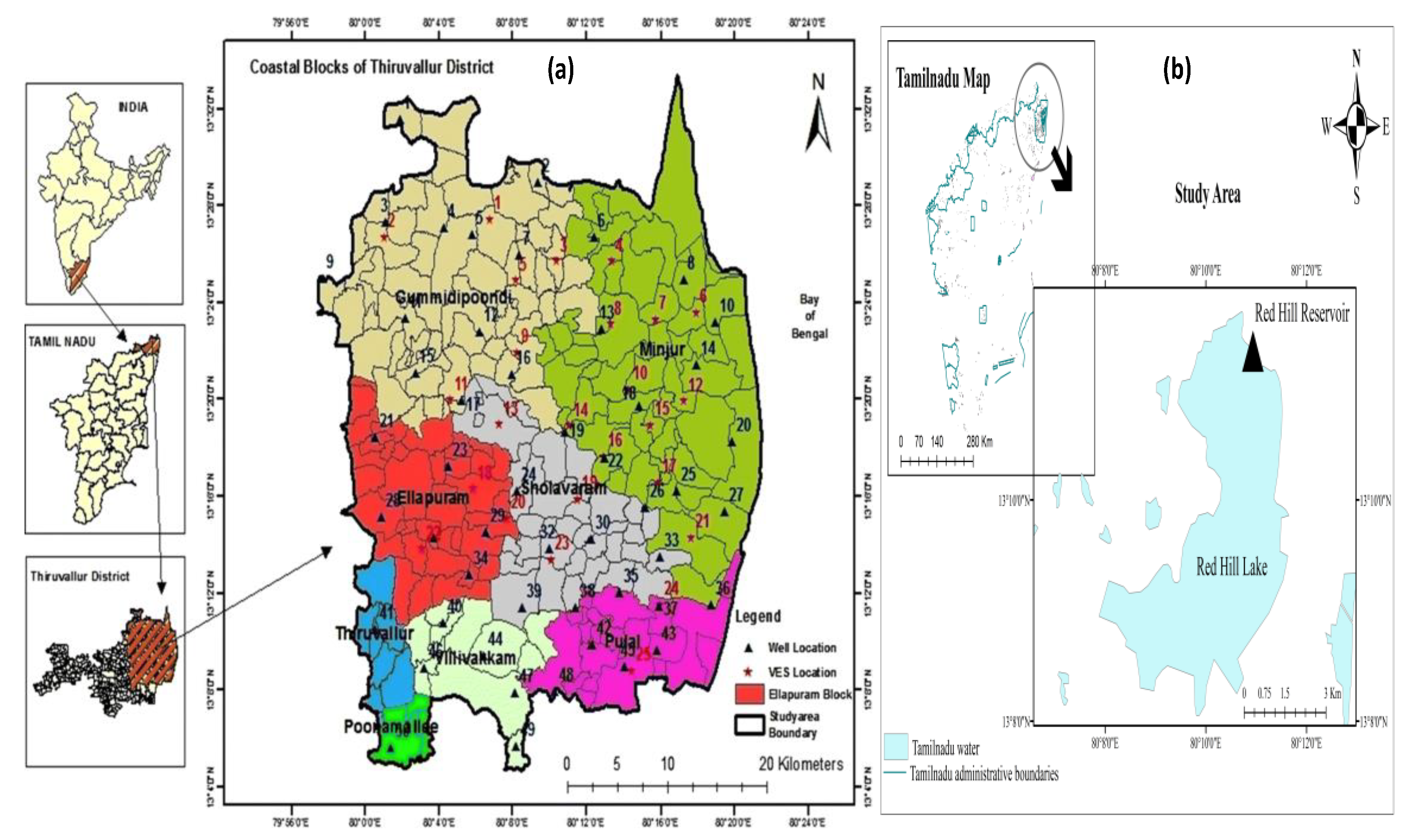
Red Hills Reservoir (RHR) is taken as the study area in this study, which is also known as the Puzhal Lake. The reservoir is located in Chennai City, Red Hills, Thiruvallur district, Tamil Nadu, South India, which is shown in Figure 2. The area is bounded by 13°11′53″ N latitude and 80°11′54″ E longitude. The reservoir is spread over an area about 20.89 km² and has a total storage capacity of 3300 million ft³ (93 million m³).

2.4. Data Collection

The daily RWL data for the RHR were collected from Chennai Water Management for the period from January 2004 to November 2020 [41]. The daily data was converted to average monthly data, which were used for developing and testing the models in the current study. The monthly average RWL for the RHR is shown in Figure 3. As can be seen from the figure, the highest amount of RWL was nearly 32 million ft³ in January 2011, whereas the lowest amount was found to be 0 in September 2004.

2.5. Seasonal ARIMA (SARIMA) Model

In the 1930s and 1940s, an electrical engineer called Norbert Wiener et al. created the ARIMA idea later named the well-known Box–Jenkins technique. The ARIMA model, also known as $\left(p,d,q\right)$ model, is a stochastic model that has been commonly used in hydrological prediction studies [42,43]. The ARIMA model is made up of three components: AR, I, and MA. The AR model denotes the link between current and previous data, the MA denotes the auto correlation frame work of error, and the I denote the series’ differencing level. It provides a time series approach towards problems by making a prediction. Peter Whittle proposed the first general version of ARMA in 1951 [44], which may be written as:

$$X_t = c+{\epsilon }_t+{{\displaystyle \sum }}_{i=1}^p{\phi }_t{X}_{t-1}+{{\displaystyle \sum }}_{i=1}^q{\theta }_i{\epsilon }_{t-i}$$

(5)

where ${\epsilon }_t$ was denoted a white noise and $\varphi$, $\theta$ were denoted the time series coefficients. Equations (6) and (7), which were presented by, show the numerical structure of AR ($p$) and MA ($q$) [45]:

AR ($p$),

$$y_t=c+{\beta }_1{y}_{t-1}+{\beta }_2{y}_{t-2}+{\beta }_3{y}_{t-3}+\cdots +{\beta }_p{y}_{t-p}+{ϵ}_t$$

(6)

This is an instance of multiple regressions with lagged $y_t$ values as predictors. It’s denoted as AR ($p$):

MA ($q$)

$$y_t=c+{ϵ}_t+{\alpha }_1{\epsilon }_{t-1}+{\alpha }_2{\epsilon }_{t-2}+{\alpha }_3{\epsilon }_{t-3} \dots +{\alpha }_q{ϵ}_{t-q}$$

(7)

ARIMA $\left(p,d,q\right)$,

$$\begin{gathered} y_t=c+{\beta }_1{y}_{t-1}+{\beta }_2{y}_{t-2}+{\beta }_3{y}_{t-3}+\cdots +{\beta }_p{y}_{t-p}{ϵ}_t+{\alpha }_1{\epsilon }_{t-1}+{\alpha }_2{\epsilon }_{t-2}+ \\ {\alpha }_3{\epsilon }_{t-3} \cdots +{\alpha }_q{ϵ}_{t-q} \end{gathered}$$

(8)

the term $\beta$ coming from AR and $\epsilon$ the error terms coming from MA model.

The SARIMA was used to eliminate seasonal variance characteristics of data via seasonal differences [46]. They’re the same as in the ARIMA model, as follows:

$p$: Order of trend autoregression;

$d$: Order of trend difference;

$q$: Order of trend moving average.

There are four seasonal components that must be adjusted that are not part of ARIMA:

$P$: Order of Seasonal autoregressive;

$D$: Order of Seasonal difference;

$Q$: Order of Seasonal moving average;

m: A single seasonal period’s number of time steps.

The general equations for the SARIMA model can be defined by Equations (9)–(13):

$${\varphi }_p\left(L\right){\mathsf{\Phi }}_p\left(L^s\right){\left(1-L\right)}^d{\left(1-L^s\right)}^D{Z}_t={\theta }_q\left(L\right){\mathsf{\Theta }}_Q\left(L^s\right){\epsilon }_t$$

(9)

$${\varphi }_p\left(L\right)=1-{\varphi }_{1}L-{\varphi }_2{L}^2-\cdots -{\varphi }_p{L}^P$$

(10)

$${\theta }_q\left(L\right)=1-{\theta }_{1}L-{\theta }_2{L}^2-\cdots -{\theta }_q{L}^q$$

(11)

$${\mathsf{\Phi }}_p\left(L^s\right)=1-{\mathsf{\Phi }}_S\left(L^S\right)-{\mathsf{\Phi }}_{2S}\left(L^{2S}\right)-\cdots -{\mathsf{\Phi }}_{PS}\left(L^{PS}\right)$$

(12)

$${\mathsf{\Theta }}_Q\left(L^S\right)=1-{\mathsf{\Theta }}_S{L}^S-{\mathsf{\Theta }}_{2S}{L}^{2S}-\cdots -{\mathsf{\Theta }}_{QS}{L}^{QS}$$

(13)

where, $Z_t$stands for the observed value and ${\epsilon }_t$ stands for the lagged error at time $t$; $L$ (lag operator) defined by:

$$\begin{gathered} L^k{Z}_t=Z_{t-k }; {\varphi }_p\left(p=1,2,\dots ,p\right), {\mathsf{\Phi }}_p\left(P=1,2,\dots ,P\right), \\ {\theta }_q\left(q=1,2,\dots ,q\right), {\mathsf{\Theta }}_q\left(Q=1,2,\dots ,Q\right) \end{gathered}$$

(14)

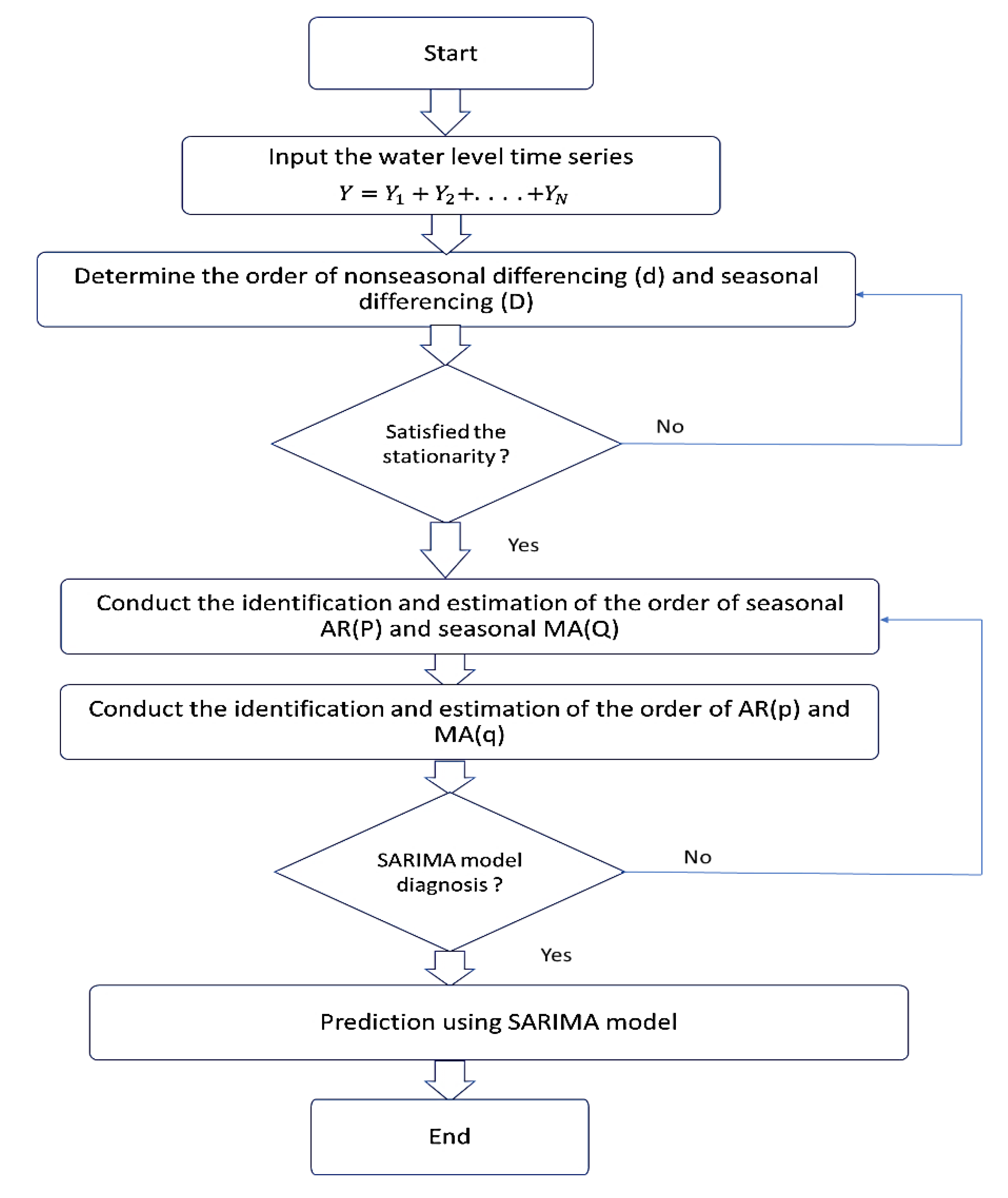
The orders of autoregressive and moving average were represented by $p$ and $q$, respectively. $P$ and $Q$ indicate the seasonal autoregressive and seasonal moving average orders, accordingly. $S$ stands for seasonal length, whereas $d$ and $D$ stand for difference order and seasonal difference, respectively. Figure 4 shows the flowchart of SARIMA model.

The mean, variance, and autocorrelation functions of the data were tested for stationarity with respect to time as a prerequisite for using the SARIMA model. ${\epsilon }_t$ (random error) was also made independent and distributed similarly to a standard zero-mean dispersion. Higher weights were regarded as indicators of a better prediction model when the SARIMA model was tested for weights [47,48]. After the selection of weights, the SARIMA model was modelled in four stages including: (i) stationarity check; (ii) identification and estimation stage; (iii) diagnosis stage; and (iv) prediction stage. In stage one, the time series data were checked for stationarity. The stationarity of data was checked followed by the Augmented Dickey Fuller (ADF) test, which examines a time series for the null hypothesis of the existence of a unit root [49]. ADF’s mathematical expression is as follows:

$$\Delta y=\alpha +\beta t+\gamma y_{t-1}+{\delta }_1\Delta y_{t-1}+\cdots +{\delta }_{p-1}\Delta y_{t-p+1}+{ϵ}_t$$

(15)

where $\alpha$ is constant, $\beta$ is time trend coefficient, $p$ lag order, and ${ϵ}_t$ is the error term. Before executing the test for the null hypothesis $\gamma =0$, the appropriate lags of order $p$ were selected. If the time series is non-stationary, stationarity can be obtained by regressing or differencing the data until it becomes stationary [50]. Non-seasonal and seasonal differencing are the two types of differencing with order $d$. Seasonal difference is a technique for removing seasonal components from data and by eliminating trend characteristics from the data, the non-seasonal difference aims to address data instability [51]. This can be achieved by determining the order of the SARIMA model, estimating unknown parameters, accumulating model candidates with a p-value of less than 0.05, and evaluating the goodness of fit on the anticipated errors; then, predicting a value in the future using the data that is available. To establish the ordering of the SARIMA, ACF and PACF charts were required [52].

2.6. ANN Model

The capacity of an artificial neural network is to represent complicated nonlinear relationships [48,53,54,55,56,57]. One of the most extensive ANN for time series modelling and prediction is the multilayer perceptron, especially individuals with one hidden layer. A network of three layers of functioning is linked by acyclic linkages. The mathematical equation between the output ($y_t$) and the inputs ($y_{t-i}$, …, $y_{t-p}$) as follows:

$$y_t=w_0+{\displaystyle \sum }_{j=1}^Q{w}_{g}g \left(w_{0j}+{\displaystyle \sum }_{i=1}^p{w}_{i,j}{y}_{t-i}\right)+e_t$$

(16)

where $w_{i,j}$ ($i=0, 1, 2 , \dots , P,j =1, 2, \dots , Q)$ and $w_j \left(j=0, 1, 2, \dots , Q\right)$ stands for model parameters, which are also known as connection weights; the number of input nodes is indicated by $P$; and the number of hidden nodes is represented by $Q$. For hidden layers, the sigmoid function is frequently employed transfer function, that is:

$$Sig\left(x\right)=\frac{1}{1+\exp \left(-x\right)}$$

(17)

$$y_t=f\left(y_{t-i} , \dots , y_{t-P}, W\right)+e_t$$

(18)

As a result, the ANN model of (18) conducts mapping from historical data to projected values $y_t$, i.e.,:

where $f\left(.\right)$ is a function based on the network structure and connection weights and $W$ is a vector containing all parameters. In the output layer, the formulation (18) implies one output node, which is generally employed for a step-ahead prediction. The basic network represented by (18) is remarkably strong in that it can estimate any function when the neurons of hidden nodes $\left(Q\right)$ are high enough [58]. In out-of-sample predictions, a basic network layout with a modest number of hidden nodes frequently works effectively. This might be related to the over-fitting phenomenon that occurs frequently in neural network models [59].

As $Q$ is data dependent, there is no methodical procedure for determining this parameter. The selection of the number of lagged observations, $P$, and the dimensionality of the input vector is another essential part in ANN modelling of a time series [59], in addition to determining the adequate number of hidden nodes. Because it determines the (nonlinear) autocorrelation frameworks of the time series, it is likely the most critical parameter to estimate in an ANN model. There is, nevertheless, no hypothesis that can be utilized to assist in $P$ selection. As a result, studies are frequently undertaken to find a suitable $P$ and $Q$.

2.7. Hybrid SARIMA-ANN Model

The SARIMA models’ approximation of complicated nonlinear issues may not be acceptable. The use of artificial neural networks to represent linear issues has generated mixed results. Denton et al. [60], for example, demonstrated that when the data contain outliers or multicollinearity, neural networks outperformed linear regression algorithms considerably. The effectiveness of ANNs for linear regression issues is similarly influenced by sample size and noise level, according to Markham et al. [61]. As a consequence, employing ANN is unwise since it is unfeasible to adequately comprehend the characteristics of data in a real situation. A hybrid technique which merges the linear and nonlinear skills might be a useful strategy in practice. In the first phase, the SARIMA model is employed to extract the linear component of the time series. The residuals of SARIMA and the lagged data are then employed as input for statistical ML techniques throughout the second step. Lastly, predictions were estimated using best suited model in the third step. The following sections go into the specifics of these steps:

$$y_t=L_t+N_t$$

(19)

where $L_t$ represents the linear element and $N_t$ indicates the nonlinear component, these two factors must be calculated based on the data. At first, the SARIMA model was employed as the linear module, and then the linear model’s residual was determined from the model. Let $e_t$ stand for the linear model’s residual at time $t$, then:

$$e_t=y_t+{\widehat{L}}_t$$

(20)

where${\widehat{L}}_t$ is the calculated relationship’s prediction value for time $t$. The diagnosis of the sufficiency of linear models relies heavily on residuals. If there are still linear correlation patterns in the residuals, a linear model is insufficient. Residual analysis, on the other hand, is unable to find any nonlinear correlations. In reality, no universal diagnostic statistics for nonlinear auto correlation connections exist at this time. As a result, if the model passes diagnostic testing, it might still be insufficient since nonlinear interactions have not been adequately represented. The SARIMA’s restriction will be shown by any major nonlinear pattern in the residuals. Modeling residuals with ANNs may be used to investigate nonlinear linkages. For residuals, an ANN model will be used as follows:

$$e_t=f\left(e_{t-1},e_{t-2},\dots ,e_{t-n}\right)+{\epsilon }_t$$

(21)

where$f$ is non-linear function and ${\epsilon }_t$ is the random error. It’s worth mentioning that if model $f$ isn’t adequate, the error term isn’t always random. As a consequence, it’s crucial to have the right model. The prediction from (18) will be denoted as ${\widehat{N}}_t$, and the combined prediction will be:

$${\widehat{y}}_t={\widehat{L}}_t+{\widehat{N}}_t$$

(22)

In summary, the suggested hybrid technique comprises of two parts. During the first phase, the SARIMA was utilized to investigate the linear component of the problem. In the second phase, the residuals from the SARIMA model were modelled by ANN. The residuals of the linear model will contain information on the nonlinearity because the SARIMA model could not account for data’s nonlinearity. The findings of the neural network may be utilized to anticipate the SARIMA model’s error terms. In identifying diverse patterns, the hybrid model uses the unique features and strengths of both the SARIMA and ANN models. This might be beneficial to analyze linear and nonlinear trends independently employing various techniques and then integrate the predictions to enhance overall modelling and prediction performance.

Figure 5 shows the SARIMA and ANN hybrid model in which the SARIMA model is combined with the ANN model. As described earlier, in developing SARIMA and ANN models, subjective interpretation of the order and model appropriateness is often needed. In the hybrid technique, it is conceivable that suboptimal models will be utilized. Box–Jenkins technique, for example, relies on low order auto correlation. Even if substantial auto correlations of higher order exist, the model was regarded acceptable if low order auto correlations were insignificant. The hybrid model’s usefulness may not be blemished by this suboptimality. In 1989, Granger pointed out that the component model in a hybrid model should be suboptimal in order for the hybrid model to generate the enhanced prediction [62,63].

2.8. Performance Evaluation of the Models

The outcomes of the SARIMA, ANN, and SARIMA–ANN hybrid models were monthly RWL of Red Hills Reservoir for the January 2004–November 2020 period. The predicted values obtained by the models were compared with the actual dataset. Several statistical performance indicators, including RMSE, MAE, MAPE, and $R^2$ (Equations (23)–(26)) were used to evaluate the performance of each model. A lower value of MAE, RMSE, and MAPE indicate a good correlation between the observed and predicted datasets. The value of $R^2$ closer to 1 demonstrates a good correlation between the observed and predicted data sets:

$$MAE=\frac{1}{n} {\displaystyle \sum }_{i=1}^n\left|O_i-P_i\right|$$

(23)

$$RMSE=\sqrt{\frac{{{\displaystyle \sum }}_{i=1}^n{\left(O_i-P_i\right)}^2}{n}}$$

(24)

$$MAPE=\frac{1}{n} {\displaystyle \sum }_{t=1}^n\left|\frac{\left(O_i-P_i\right)}{O_i}\right|\times 100$$

(25)

$$\begin{array}{c}{R}^2=1-\frac{{{\displaystyle \sum }}_{i=1}^n{\left(O_i-P_i\right)}^2}{{{\displaystyle \sum }}_{i=1}^n{\left(O_i- \widehat{P_i}\right)}^2} \end{array}$$

(26)

Here, $O_i$ represents the observations, $P_i$ represents the predictions at each time step, and n represents total time step numbers.

3. Results

The entire obtained data were separated into two portions for training and testing of the model in order to assess and compare the adopted modelling techniques. The training datasets were those from January 2004 to March 2017, accounting for 80% of the dataset, while the remaining dataset (20%) were used for model testing purpose.

To anticipate the SARIMA model, firstly we had to analyze the fluctuation of the RWL data based on Figure 2. The approach of the SARIMA model was carried out in three phases. First, the difference’s requirement was identified, a stationarity test was accomplished for this reason. The samples were stationary adjusted through differencing, and then SARIMA $p,d,q,m$ and $P,D,Q$ parameters were identified using ACF plots and PACF.

Step 1: Stationarity test of the Data

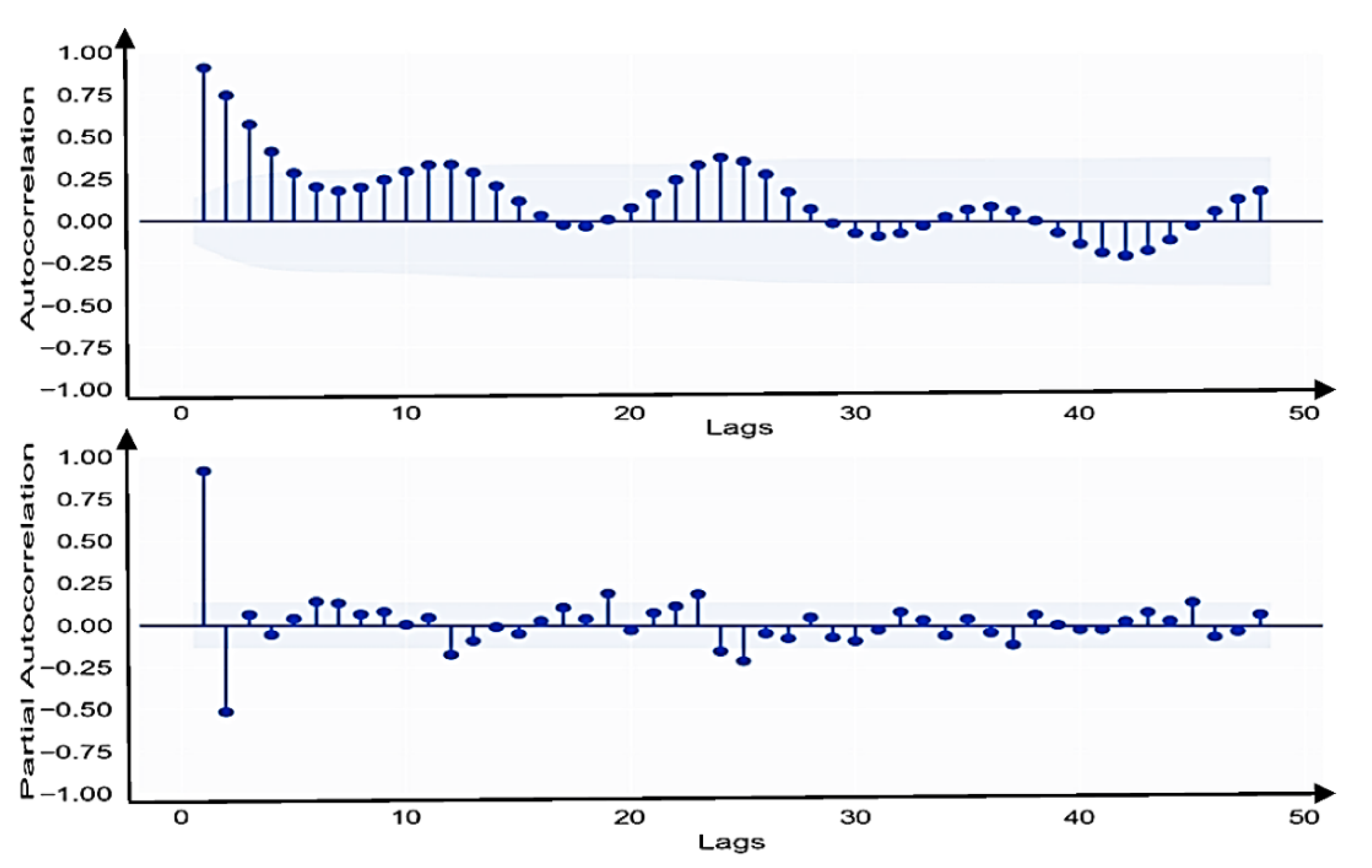
The ADF test indicates that the null hypothesis that the dataset has a unit root (non-stationary) at the 5% significance level may be rejected. According to the ACF graph (Figure 6), the seasonally differenced trend shows significant spikes in negative values at the 1st lag, and ACF shuts out after that for the non-seasonal element.

Due to seasonal influences, the ACF exhibits strong spikes at numerous lags that demonstrate a periodic order across 12 months, non-seasonal differencing is thus unnecessary, whereas seasonal differencing is essential due to seasonal stationarity.

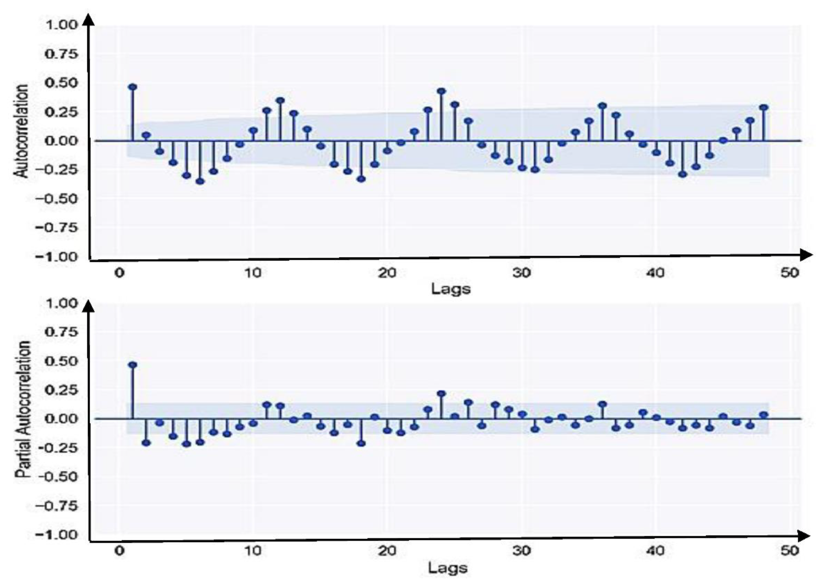
Furthermore, substantial spikes were noticed after first order differencing at intervals of every 12 months (12th, 24th, 36th lags …) on the ACF plot in Figure 7. As a result, to reduce seasonality, a seasonal differencing technique continued till third order differencing. A chart of ACF and PACF with seasonal differences is shown in Figure 8 after third order seasonal differencing.

Step 2: Model Identification

This stage is to estimate the suitable values of $p, d, \mathrm{and} q$ employing correlogram and partial correlogram and ADF Test. The preliminary model’s order was determined using the ACF and PACF. The ACF exhibits strong spikes at numerous lags, which demonstrate a periodic sequence over 12 months due to seasonal impacts, as seen by the correlogram. At many lags, the PACF shows substantial increases; therefore, the model might be a SARIMA model.

The observed RWL samples were subjected to seasonal differencing $\left(D=3\right)$ in order to create a time series that was seasonally stationary. For future exploration, SARIMA $\left(p, 0, q\right) \left(P, 3, Q\right)12$ are recommended. Initial, parameters of $p, q, P \mathrm{and} Q$ were identified by ACF and PACF plots (Figure 5).

The seasonal component of ACF displays a positive substantial spike at the 12th and 24th lags. As a result, for model identifier, two seasonal (SMA) and one non-seasonal MA values are recommended. In the same way, for PACF, there were no seasonal or non-seasonal significant spikes detected. Hence, zero AR for non-seasonal and zero seasonal (SAR) are recommended for inclusion in the SARIMA model. As a consequence, SARIMA (0, 0, 1) (0, 3, 2)₁₂ was identified for further evaluation.

Step 3: Parameter Estimation

The parameters of the AR and MA were estimated in this stage.

Here the parameter estimates in

Table 1. Parameter estimates for SARIMA (0,0,1) (0,3,2) model.

Parameter	${\mathit{\theta }}_1$	${\mathbf{\Theta }}_1$	${\mathbf{\Theta }}_2$
Value	0.7993	−1.5737	0.5760

Explanations: ${\theta }_1$ = MA parameter of non-seasonal components, ${\mathsf{\Theta }}_1$,${\mathsf{\Theta }}_2$ = MA parameters of seasonal components.

and the performance values are shown in

Table 2. Performance values of selected models.

Akaike information criterion	2010.938
Bayesian information criterion	2022.283
Hannan-Quinn criterion	2015.547
Ljung-Box	27.74
Heteroskedasticity	2.00

for SARIMA model.

Step 4: Diagnostic Checking

At this stage, residual’s diagnosis, standard residual, histogram plus estimated density, normal $Q-Q$, and correlogram were checked to analyze the model.

Figure 9a shows that the residual errors seem to fluctuate around a mean of zero and have a uniform variance. Figure 9b illustrates the density plot. It suggests a normal distribution with a mean zero. Figure 9c demonstrates that all the dots fall closely with the red line. Any significant deviations would imply that the distribution is skewed. Figure 9d reveals that the residual errors are not autocorrelated.

Figure 10 shows the ACF and PACF plots of residuals for RWL dataset. The ACF and PACF of the residual is showing inadequate results and the presence of autocorrelation in residuals may be determined employing the Durbin Watson (DW) test. The DW value should be in the range of 1.5 and 2.5 [64,65]; here, the value is 0.99, which indicates that the SARIMA (0, 0, 1) (0, 3, 2)12 model is not well fitted for prediction. The alternative which used to resolve the problem is building a residual model of SARIMA using ANN which is no regression assumption.

The information about the neural network architecture shows that network has an input layer, two hidden layers with 512 and 4 nodes, and an output layer with one output node. For the best network structure, an ANN should be used with the appropriate number of hidden layers and neurons in each hidden layer. The enumeration approach is based on least MSE used in the ANN modelling to discover the best number of layers and associated neurons in each hidden layer. All of the sample data have to transform into a value between 0 and 1 because of the activation function which is used in artificial neural network is sigmoid function. The error is the sum-of-squares error because identity and activation function are applied to the output layer. Initialization, feed-forward, error assessment, propagation, and adjustment are the learning methods of the artificial neural network. An optimised network of topology 2-512-4-1 was determined to be superior to the other studied network topologies based on MSE criteria. The training cycle was set at 500 epochs, while bath size and validation split are 4 and 0.2, respectively. A neural network is typically initialized using random weights during the initialization process [66].

Figure 11 reveals the SARIMA residuals plot of RWL dataset employed to test the existence of nonlinearity. The best selected SARIMA, ANN, and SARIMA–ANN models were compared based on MAE, MAPE, RMSE, and $R^2$ values using Equations (23)–(26). The comparison results are given in

Table 3. Evaluation results for SARIMA, ANN and SARIMA-ANN models.

Model	MAE	MAPE	RMSE	${\mathit{R}}^2$
SARIMA	798.10	79,810.15	891.994	0.30
ANN	660.32	66,032.258	806.062	0.51
SARIMA-ANN	343.23	34,323.06	430.728	0.84

. The results show that the SARIMA–ANN model performed better than single SARIMA and ANN models in prediction of data, with an $R^2$ value of 0.84, MAE value of 328.69, MAPE value of 32,868.51, MSE value of 174,043.217, and RMSE value of 417.185. Furthermore, the RWL number’s projected value is almost identical to its actual value.

Figure 12, Figure 13 and Figure 14 shows the results for predicted RWL using SARIMA, ANN, and hybrid SARIMA–ANN models, respectively. The graphs shown that while applying ANN alone in the test dataset, the performance is worse comparing to the SARIMA and SARIMA–ANN models. It can be observed that the predicted monthly RWL obtained from the fitted SARIMA–ANN model is matching closely with the pattern of the curve of actual RWL.

4. Discussions

When it comes to river systems, India is a wealthy country. The Aravalli, Ganges, Brahmaputra, and Indus are four significant river systems in India, each with a substantial catchment area and drainage density. All of these river systems have several tributaries that run the length and width of India, making it more vulnerable to flooding [67]. Consequently, during the years 1987 and 1993, the cycle of floods followed by severe drought and its impact on water shortage in Chennai was at its peak. A severe drought struck Chennai City in 1986. Only 40% of the rainfall was reported and 17% of the total available water in the city’s three lakes was used. Legislation to regulate the exploitation of groundwater was required. The groundwater level in Chennai was roughly 8 m deep in 1988, but it rose to 4.08 m in 2007.

From 1988 through 1996, there was increasing commercial exploitation. Proactive detection of water intensity in a given location is always useful for planning with scarce resources and implementing effective intervention techniques. A high-quality water level prediction is required to optimize the net benefits of water management. This surface water is critical to the region’s socioeconomic development and expansion. Water infrastructure development, floods, and droughts all have an impact on industrial operations, necessitating smart resource management. Precision water level prediction not only decreases the danger of mis-operation and the likelihood of damage, but it also boosts earnings. There is a lack of statistical computational analysis that might use prediction models to anticipate water increase in Chennai. In such cases, advanced computational models, such as SARIMA and ANN were chosen with the goal of predicting water level and, as a result, filling the gap in the specific region.

The selected models for the water level prediction in this study could be used confidently to estimate the water level in the Red Hills Reservoir. The results obtained in the present study are in validation of other previous studies that were performed for the prediction of water level in India using ANN, such as M.Y.A. Khan et al. [68], that has put the application of ANN into use for the prediction of water level for the Ramganga river, which suggests the prediction accuracy of 93.42%. Additionally, machine learning techniques, such as wavelet and support vector machine implementation has also been performed by Yadav et al. [69] to predict the daily water level of Loktak lake (India). The prediction accuracy for accumulated data in this study was found to be higher than the original data series based on the performance evaluation using RMSE, because it accounted for the past data for analysis that increased the prediction efficiency. Moreover, a hybrid system of ANN and machine learning was used to forecast the water level in Jhelum river at Sangam station of Kashmir valley in India to improve the early warning system for flood prevention. It was found that the condition of accuracy depends on previous data and forecasted values of temperature and precipitation [70].

Based on the application of previous and present studies, the conditions for the application of predicting the water level include the applicability of the past data collected, data collection techniques, and a hybrid prediction algorithm rather than standalone method. The accuracy of prediction of water level depends on the forecasted values of precipitation, weather conditions, and location. Therefore, the short-term prediction results are more promising than the long-term prediction.

In other words, monthly water level data may be examined without any adjustments to meteorological data, such as temperature, precipitation, wind speed, humidity, sun hours and UV index, and amount of the location, which would be the reason for its global generalization, because multivariate data is not required to assess the prediction of water level data. Apart from the findings, it will be impressive to observe if the hybrid strategy is useful in crucial conditions, such as when the water level rises dramatically (suggesting a peak in water level). The visual comparisons of all approaches for water level prediction are shown in Figure 12, Figure 13 and Figure 14. The Figures show that the SARIMA and ANN hybrid model could represent the trend of the actual data fairly well, despite the fact that single techniques do not function effectively in any of these circumstances. It is also worth mentioning that the results are solely applicable to the examined region owing to the statistical application of the analysis. As a result, due to the changing nature of statistical data, any model that successfully predicts reservoir water level data for this research may not be useful for other areas. To put it another way, the SARIMA and ANN hybrid models utilized in this work for reservoir water level prediction in various areas may differ due to regional differences. The type of data, such as seasonality, residuals, autocorrelation, and the data’s explanatory power, would have a significant impact on the prediction utilizing SARIMA and ANN for any region.

5. Conclusions

The probabilistic aspect of RWL prediction is investigated in this study using a hybrid model, SARIMA and ANN model for the Red Hills Reservoir (RHR). Time series data originating from various applications, in general, comprise both linear and nonlinear variations. Linear SARIMA and nonlinear ANN models cannot individually take out consequence data accurately. Hybrid models, which combine the strengths of SARIMA and ANN models, are better than individual types of models as they are capable of exploiting the advantages of both types of models simultaneously. The results show that the hybrid SARIMA–ANN model performed better than the SARIMA and ANN model for RHR in the RWL prediction. The prediction from the hybrid model is obtained by adding the predicting values from the two individual models. Thus, the hybrid model proposed in the present paper becomes a simple and accurate prediction model in many applications.

6. Limitations and Future Scope

A mix of linear and nonlinear models were utilized in this research. In their respective linear or nonlinear domains, both SARIMA and ANN models have great success in the particular area. Neither of them, however, are universal paradigms that can be used in all situations. It is possible that the SARIMA models’ approximation of complicated nonlinear issues is insufficient. ANNs, on the other hand, have had inconsistent success when used to simulate linear issues. To improve model accuracy, most external parameters, including meteorological data, such as temperature, precipitation, wind speed, humidity, sun hours, and UV index should be added with the passage of time. The results of this study could be a good reference for the facilitators and decision-making stakeholders by performing predictions in a quick and easy way by incorporating the methodology adopted in this study. Because, unlike other techniques for prediction, this approach does not require a colossal set of data that is collected through epidemiological retrospective information. For future studies, meteorological elements should be used as independent variables to increase the accuracy of anticipated findings. This research might be used for such locations where natural disasters cause the majority of water shortages.