Renewable Thermal Energy Driven Desalination Process for a Sustainable Management of Reverse Osmosis Reject Water

Abstract

A sustainable circular economy involves designing and promoting products with the least environmental impact. This research presents an experimental performance investigation of direct contact membrane distillation with feed approaching supersaturation salinity, which can be useful for the sustainable management of reverse osmosis reject water. Traditionally, reject water from the reverse osmosis systems is discharged in the sea or in the source water body. The reinjection of high salinity reject water into the sea has the potential to put the local sea environment at risk. This paper presents a design of a solar membrane distillation system that can achieve close to zero liquid discharge. The theoretical and experimental analysis on the performance of the lab scale close to zero liquid discharge system that produces supersaturated brine is studied. The lab-based experiments were conducted at boundary conditions, which were close to the real-world conditions where feed water temperatures ranged between 40 °C and 85 °C and the permeate water temperatures ranged between 5 °C and 20 °C. The feed water was supplied at salinity between 70,000 ppm to 110,000 ppm, similar to reject from reverse osmosis. The experimental results show that the maximum flux of 17.03 kg/m²·h was achieved at a feed temperature of 80 °C, a feed salinity of 10,000 ppm, a permeate temperature of 5 °C and at constant feed and a permeate flow rate of 4 L/min. Whereas for the same conditions, the theoretical mass flux was 18.23 kg/m²·h. Crystal formation was observed in the feed tank as the feed water volume reduced and the salinity increased, reaching close to 308,000 ppm TDS. At this condition, the mass flux approached close to zero due to crystallisation on the membrane surface. This study provides advice on the practical limitations for the use of membrane distillation to achieve close to zero liquid discharge.

1. Introduction

There remain major concerns over the environmental impacts of reverse osmosis reject water. To address these concerns, some researchers have begun to align their R&D efforts with the sustainable circular economy principles: Reduce, Reuse, Recycle and Replace [1,2,3]. Desalination is a sustainable solution to water shortage. Over the past three decades, desalination has shown to be the promising solution to water scarcity, being able to deliver a sustainable water supply. The global installed desalination capacity is more than 86 million m³/day. While more than 40% of the global installation capacity is found in the Gulf region and North Africa, interest in desalination has been growing in Australia, Asia and America [4].

Reverse osmosis (RO) and thermal desalination processes such as multistage flash and multi effect distillation have been the main desalination processes used worldwide. However, these methods require a high and considerable amount of energy to process [5]. Moreover, normal desalination processes in a general and reverse osmosis process in particular have a high concentrated disposal, with salinities around 70,000 ppm [6], while the average seawater salinity is around 35,000 ppm. Such rejection is a serious threat to the environment, as it can affect the temperature, turbidity and salinity in the discharge area of the sea [7]. Additionally, chemicals used in pre-treatment processes for desalination can cause toxic contaminations, which will cause fish migration and the presence of harmful algae. Another issue that is faced while disposing the brine from desalination plants is the pipe leakage that can happen and contaminate the land [8]. Considering these facts and figures, conventional desalination processes demand to be modified or retrofitted with a Zero Liquid Discharge (ZLD) system that can recover more fresh water from the reject water and produce solid crystalline salt, which could help address multiple problems such as the environment crisis, the water crisis and, in some cases, the critical mineral crisis in an approach that is similar to the circular economy approach.

Membrane distillation (MD) process can provide nearly 100% salt and non-volatile solute rejections; besides, it can operate at high salinities near saturation. MD can also operate at low pressures and temperature. As MD requires can operate at less than 100 °C heat source, the system can be coupled with a low temperature renewable energy source [9,10,11,12,13]. Therefore, MD can be considered as the optimum solution for both the water crisis and the management of brine discharge from conventional desalination [14,15,16].

Membrane distillation combines the benefits of phase change separation and the use of a hydrophobic membrane that allows only vapor to pass through it [17]. The driving force for the MD process is the temperature difference across the membrane surfaces [9,13,18,19]. This advantageous system is very beneficial since it provides nearly 100% salt and non-volatile solute rejections [9,10,11,12]. MD is also applicable with a selection of feed water sources including seawater [20], wastewater [21,22] and brackish water [23].

There exists a variation of MD configurations utilized to allow vapor molecules to migrate through the hydrophobic membrane pores and condensate in the permeate side. The main difference between the configurations is the state of the permeate side [10]. In this study, Direct Contact Membrane Distillation (DCMD) configuration is used for its simplicity [24,25,26]. In this process, both sides of the hydrophobic membrane come in direct contact with liquid state feed water and cold water. Water vapor from the feed side travels through the pores in the hydrophobic membrane due to the saturation pressure difference across the membrane generated by the temperature gradient. Water vapour condenses as it comes in direct contact with the cold water. Figure 1 illustrates the configuration of the DCMD module.

In this paper, DCMD configuration is used to study the performance of the system at different salinities and as the feed approaches the supersaturation condition where crystallization begins.

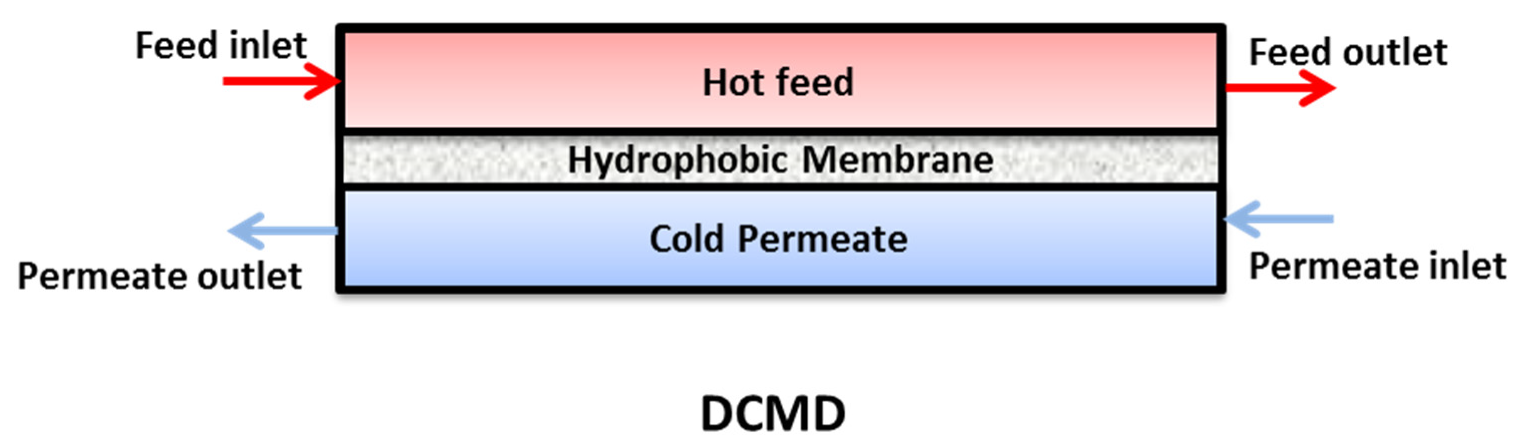
2. Theoretical Background

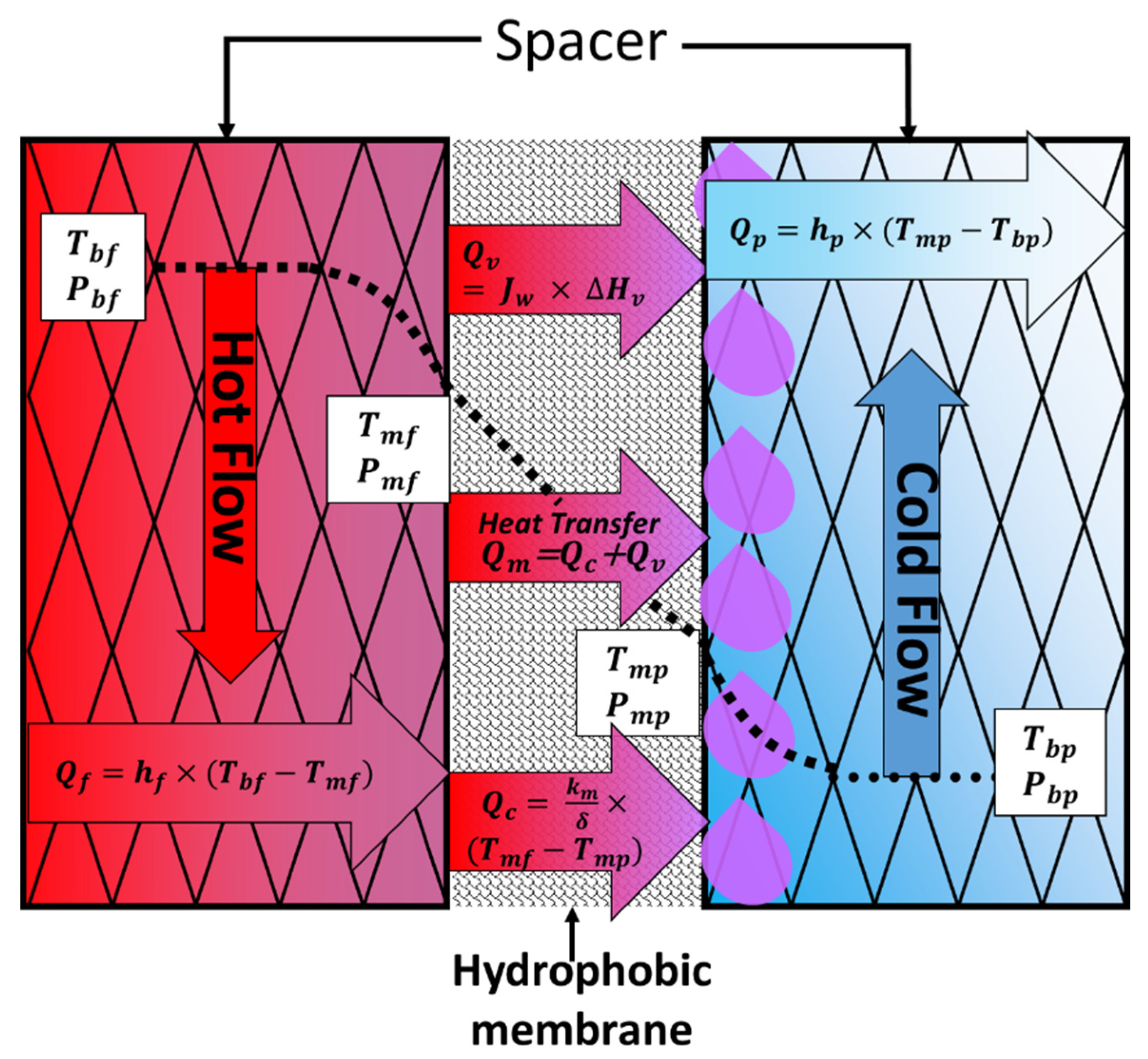
To predict and evaluate the performance of direct contact membrane distillation at different working conditions, a theoretical model has been developed. The heat and mass transfer correlations were applied to investigate the effect of the operating parameters and study the energy consumption of the system. The following assumptions are made to simplify the modelling: steady state operation, no heat losses to the surrounding and uniform pore size.

2.1. Heat Transfer

The heat transfer in MD occurs in three regions, as seen in Figure 2.

The heat transfer in the feed boundary layer (Q_f), which is the convection heat due to the temperature difference from the bulk feed temperature $T_{bf}$ and the feed temperature at the surface of the membrane $T_{mf}$.

$$Q_f=h_f\times \left(T_{bf}-T_{mf}\right)$$

(1)

where $h_f$ is the feed boundary layer heat transfer coefficient.

Heat transfer across the membrane, $Q_m$ is simply the summation of the conductive heat transfer, $Q_c$, and the latent heat of vaporisation across the membrane, $Q_v$.

$$Q_m=Q_c+Q_v$$

(2)

By using Fourier’s Law of Conduction,

$$Q_c=\left(\frac{k_m}{\delta }\right)\times \left(T_{mf}-T_{mp}\right)$$

(3)

where $k_m$ is the effective thermal conductivity of membrane, which considers both the thermal conductivity of the membrane material and the gas present in the membrane pores [19,27]. $\delta$ is the thickness of the membrane, while $T_{mf}$ and $T_{mp}$ represent the temperature of membrane surface at the feed and permeate side, respectively.

The effective thermal conductivity of the membrane can be calculated as follows.

$$k_m={\left(\left(\frac{\epsilon }{k_{gas}}\right)+\left(\frac{1-\epsilon }{k_{mem}}\right)\right)}^{-1}$$

(4)

where $k_{gas}$ is the thermal conductivity of the air trapped inside the pores of the membrane, $k_{mem}$ is the thermal conductivity of the membrane polymer and $\epsilon$ is the membrane porosity.

The evaporative heat transfer $Q_v$ can be described as the product of the molar flux $J_w$ (which will be discussed further in the following section of the mass transfer) and the enthalpy of vaporization $\Delta H_v$.

$$Q_v=J_w\times \Delta H_v$$

(5)

$$\Delta H_v=\left(\left(1.7535\times T_{mf}\right)+2024.3\right)$$

(6)

The heat transfer in the permeate boundary layer (Q_p), which is the convection heat due to the temperature difference from the membrane surface temperature $T_{mp}$ and the bulk temperature $T_{bp}$ [18,19,20,21,22,23,24,25,26,27,28,29,30,31].

$$Q_p=h_p\times \left(T_{mp}-T_{bp}\right)$$

(7)

where $h_p$ is the permeate boundary layer heat transfer coefficient.

Under a steady state condition, the whole heat transfer across the DCMD system can be written as:

$$Q_f=Q_m=Q_p$$

(8)

Equating these equations leads to determining the temperatures of membrane surfaces on both the feed and permeate side.

$$T_{mf}=\frac{k_m\times \left(T_{bp}+\frac{h_f}{h_p}\times T_{bf}\right)+\left(\delta \times \left(h_f\times T_{bf}-J_w\times \Delta H_v\right)\right)}{\left(k_m\right)+\left(h_f\times \left(\delta +\frac{k_m}{h_p}\right)\right)}$$

(9)

$$T_{mp}=\frac{k_m\times \left(T_{bf}+\frac{h_p}{h_f}\times T_{bp}\right)+\left(\delta \times \left(h_p\times T_{bp}-J_w\times \Delta H_v\right)\right)}{\left(k_m\right)+\left(h_p\times \left(\delta +\frac{k_m}{h_f}\right)\right)}$$

(10)

By using the dimensionless Nusselt number ($N_u$), the heat transfer coefficient $\left(h\right)$ can be expressed as:

$$h=\frac{N_u\times k}{D_h}$$

(11)

where $k$ is the thermal conductivity of the fluid in either the feed or permeate side and $D_h$ is the hydraulic diameter of the flow channel.

$$D_h=\frac{4\times A}{p}$$

(12)

where A is the channel cross-sectional area and p is the wetted perimeter.

Several empirical correlations can be found in the literature to determine the Nusselt number; each of them is used in a specific condition such as module type or flow regime [31,32]. For laminar flow, the Nusselt number can be calculated as follows:

$$N_u=1.86\times {\left(\frac{R_{e }\times P_r\times D_h}{L}\right)}^{0.33}$$

(13)

For turbulent flow, the correlations for the Nusselt number differ for the feed and permeate side [9,32]:

$$N_u{}_f=0.027\times {\left(R{e}_f\right)}^{0.8}\times {\left(P{r}_f\right)}^{0.4}\times {\left(\frac{{\mu }_{bf}}{{\mu }_{mf}}\right)}^{0.14}$$

(14)

$$N_u{}_p=0.027\times {\left(R{e}_p\right)}^{0.8}\times {\left(P{r}_p\right)}^{0.33}\times {\left(\frac{{\mu }_{mp}}{{\mu }_{bp}}\right)}^{0.14}$$

(15)

where $L$ is the channel length, $P_r$ and $R_e$ are the Prandtl number and Reynolds number, respectively, and are defined as:

$$P_r=\frac{\nu }{\alpha }=\frac{\mu \times C_p}{k}$$

(16)

$$R_e=\frac{\rho u D_h}{\mu }$$

(17)

where $\mu , C_p, \rho$ and $u$ are dynamic viscosity, the specific heat capacity of the fluid, flow density and flow velocity, respectively.

2.2. Mass Transfer

In DCMD, feed water vapor at the interface of the feed side and membrane surface goes through the membrane pores then condensates at the interface of the permeate cold side and membrane surface, as seen in Figure 2. The driving force for mass transfer is the vapor pressure difference at the membrane surfaces.

The theoretical permeate mass flux can be described as follows in:

$$J_w=B_m\times \Delta P_m$$

(18)

where $B_m$ is the membrane permeability and $\Delta P_m$ is the difference in vapor pressure at the trans-membrane and can be evaluated as follows:

$$\Delta P_m=P_{mf}-P_{mp}$$

(19)

where P_mf and P_mp are the transmembrane pressure one feed and permeate side, respectively. The transmembrane pressure can be calculated using the Antoine equations below [9,33]:

$$P_{mx}=\exp \left(\left(23.238\right)-\frac{3841}{T_{mx}-45}\right)$$

(20)

where P_mx is the transmembrane pressure and T_mx is the membrane surface temperature. The x can be replaced by ‘f’ for feed or ‘p’ for permeate. As the feed solution contains dissolved salt, Raoult’s law should be employed to account for the effect of the concentrate, hence the transmembrane pressure at the feed side (P_mf) will be as follows [29,34]:

$$P_{mf}=\left(1-C_s\right)P_{wmf}$$

(21)

where $C_s$ is the mole solute concentration in bulk liquid and $P_{wmf}$ is the vapor pressure at feed membrane temperature $T_{mf}$ when fresh water is used as feed and can be calculated using the Antoine Equation. Similarly, (P_mp) is the transmembrane pressure at the permeate side.

In DCMD configuration, viscous flow through the membrane is neglected as the feed and permeate streams interact with the membrane under atmospheric pressure, with the total pressure kept constant at about 1 atm [29]. This leads the combined Knudsen/ordinary diffusion mechanism to be adopted as a mass transfer mechanism, with the following equation to estimate the membrane permeability $B_m$:

$$B_m={\left[\frac{3\tau \delta }{2\epsilon r}{\left(\frac{\pi R{T}_m}{8M}\right)}^{\raisebox{1ex}{$1$}\!\left/ \!\raisebox{-1ex}{$2$}\right.}+\frac{\tau \delta }{\epsilon }\frac{P_a}{PD}\frac{R{T}_m}{M}\right]}^{-1}$$

(22)

where $\tau , \delta , \epsilon , r$ are membrane tortuosity, membrane thickness, membrane porosity and pore radius, respectively. $R$ is the gas constant, $T_m$ is the mean temperature across membrane surfaces, $M$ is the molecular weight of water molecules, $P_a$ is the air pressure in the membrane pore, P is the total pressure inside the pore and $D$ is the diffusion coefficient of water.

$T_m$ can be calculated as:

$$T_m=\frac{T_{mf}+T_{mp}}{2}$$

(23)

The value of $PD$ can be determined from the expression below, where $PD$ is in $\left(\mathrm{Pa}·{\mathrm{m}}^2/\mathrm{s}\right)$ [19,35]:

$$PD=1.895\times {10}^{-5}·T_m{}^{2.072}$$

(24)

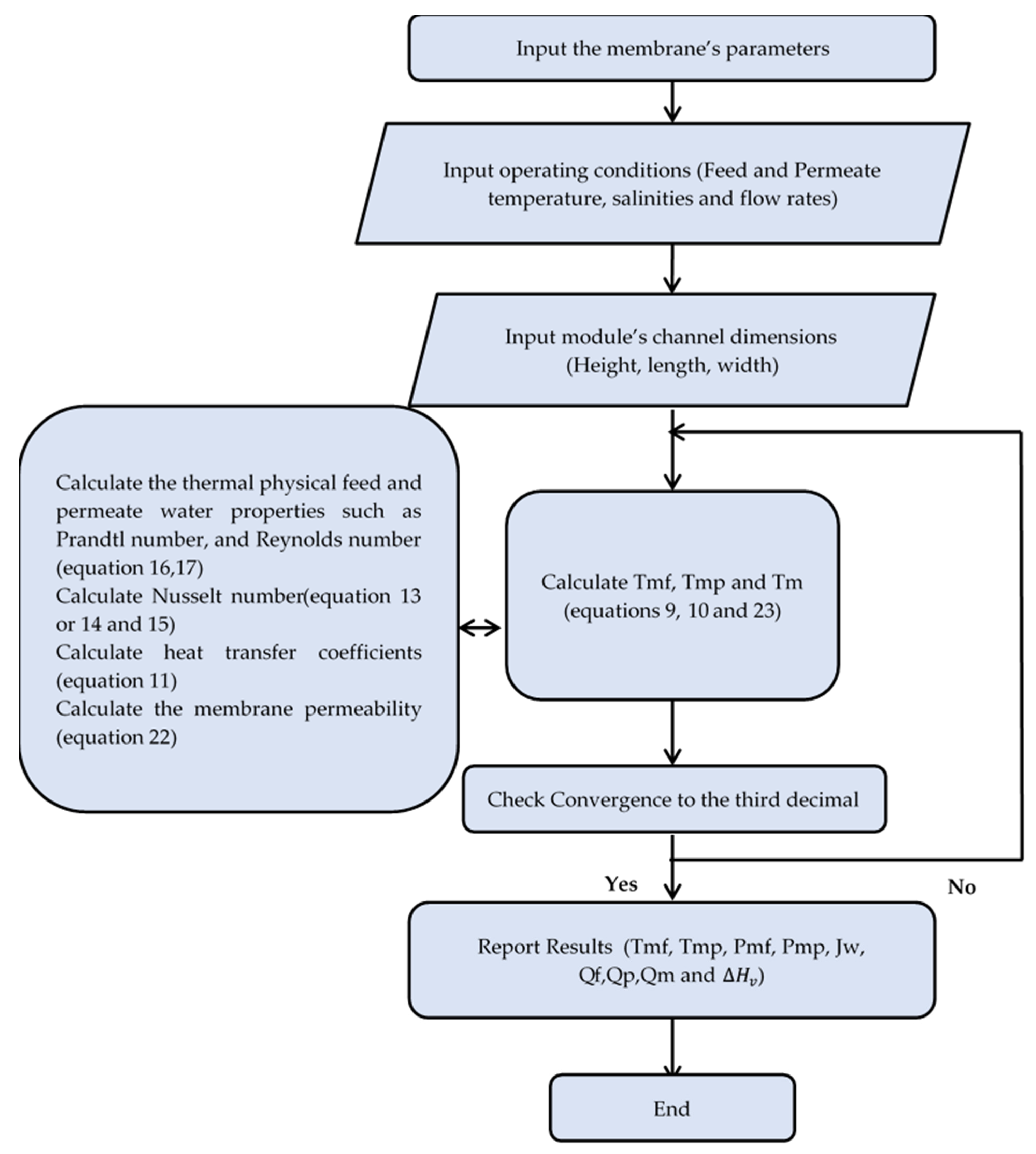
2.3. Solution Procedure

Figure 3 represents the algorithm for heat and mass transfer. Firstly, the parameters such as the membrane characteristics, the operating conditions and the channels characteristics are inputted to the software. Secondly, the software simultaneously computes the thermal physical feed and permeate water properties, the membrane permeability, the heat transfer coefficients, the membrane surface temperatures, the heat transfer rates and the mass flux in an iteration mode. Then the software checks the convergence to the third decimal. Finally, the software reports the results.

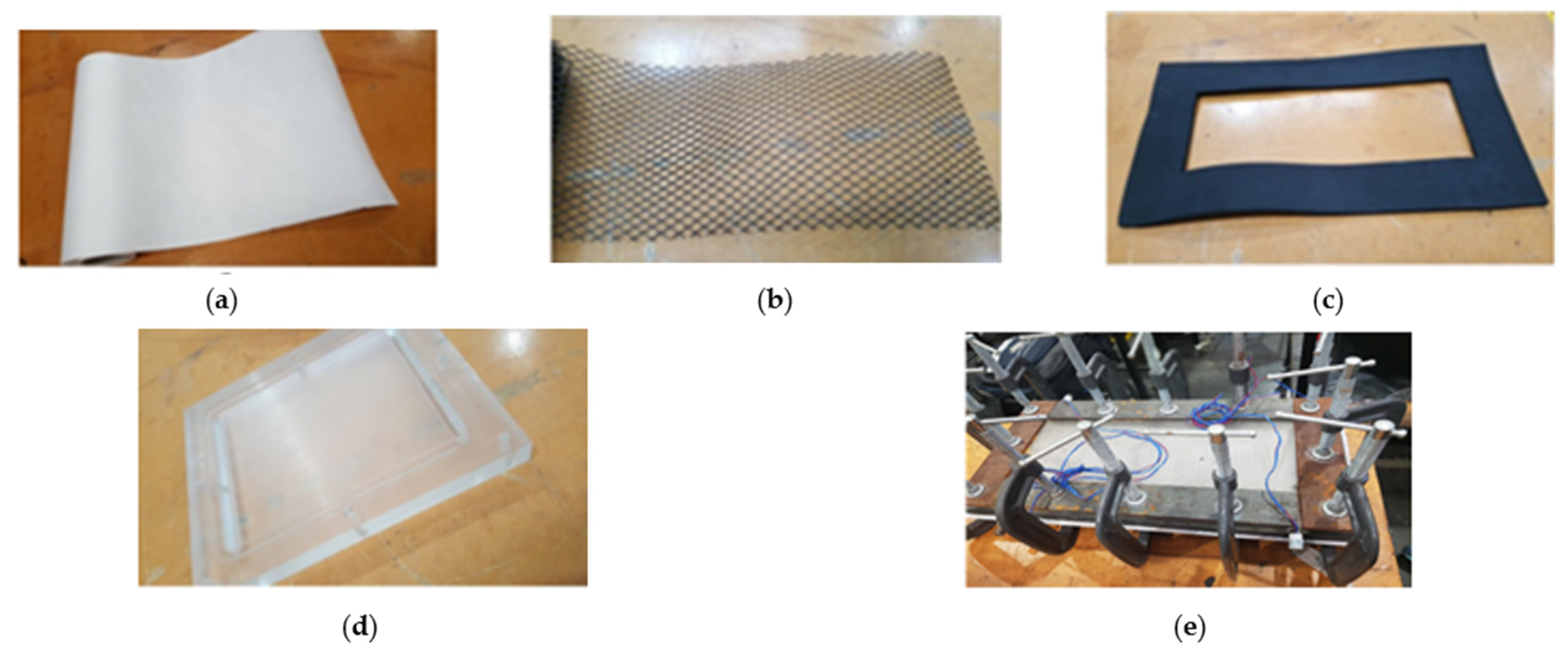
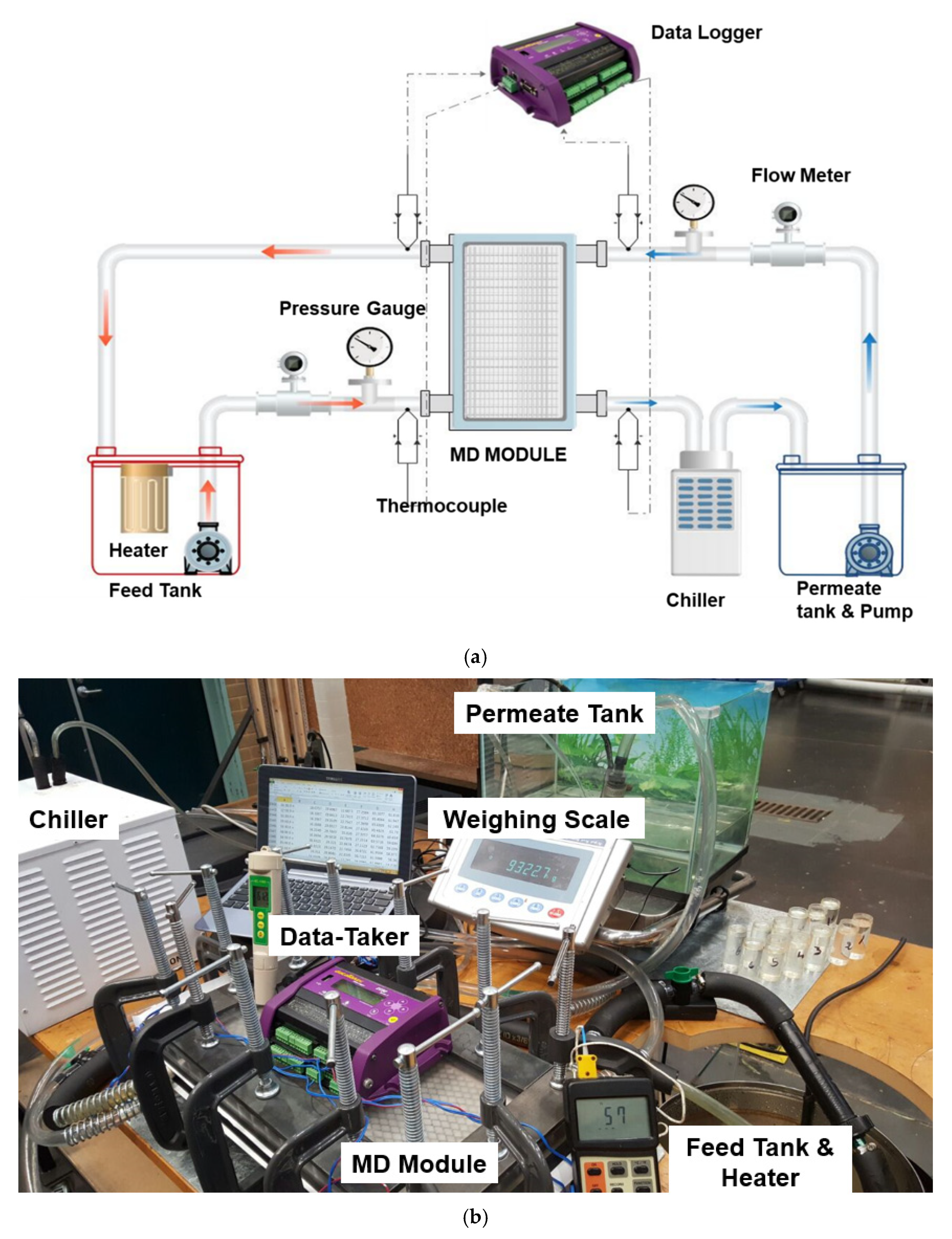
3. Experimental Procedure

3.1. Material

A plate and frame DCMD module with an effective membrane area of 0.0923 m² was designed and manufactured at the RMIT University workshop using acrylic sheets with a thickness of 25 mm. A hydrophobic PTFE membrane (85% porosity, 210 μm thickness and 0.22 μm nominal pore size) from membrane solutions was used. As shown in the figure below, to mechanically support the membrane and increase the flow turbulence, a plastic mesh structure was used at both sides of the membrane. A natural rubber gasket with 3 mm thickness from South Eastern Gaskets was used to seal the module. Finally, G claps were used to quickly assemble and disassemble the module if any modifications are required, as shown in Figure 4.

3.2. Procedure

To run the experiment, the sea water and the reject from the RO were artificially prepared by dissolving industrial raw salt in tap water. The feed water is heated up to the desired temperature with an insulated hot water urn (model: WB30-30L). At the same time, the permeate stream was maintained at the desired temperature using a 15 kW water chiller present in the RMIT thermal-fluids lab. The hot feed water and the cold permeate were pumped and circulated tangentially to the membrane using two identical submersible pumps (5–12 V Micro Hot Water Circulation Pump Brushless 3.5 M 3000 LPH). K-Flex elastomeric pipe insulations from Bunnings Warehouse were used to insulate the feed water piping. Feed and permeate water flow rates, pressures and temperatures were monitored and recorded at the inlet and outlet of both the channels. The density of feed water was measured with a handheld specific gravity/density meter (DMA 35 Anton Paar), then it was converted to salinity using Equation (25). The water at both sides was moving in a counter-current flow. Figure 5 shows the schematic and a real picture of the experimental set up. A weighing scale was used to monitor the increase in the mass of the permeate water. Further, the feed water levels and any water surface crystal formation were visually monitored.

$$S=\left[\left(\frac{\rho }{998}+\left(0.4\times {10}^{-3}\right)\left(T-293\right)-1\right)\times \frac{1}{0.65\times {10}^{-3}}\right]$$

(25)

where: $\rho$ is the fluid density at temperature T (in Kelvin) in kg/m³ and S is the salt concentration of the water kg/m³.

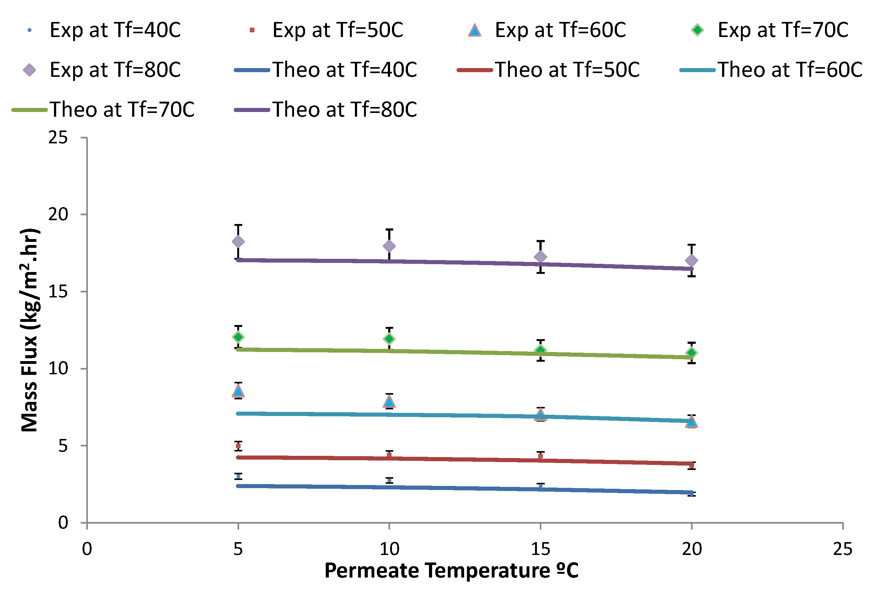
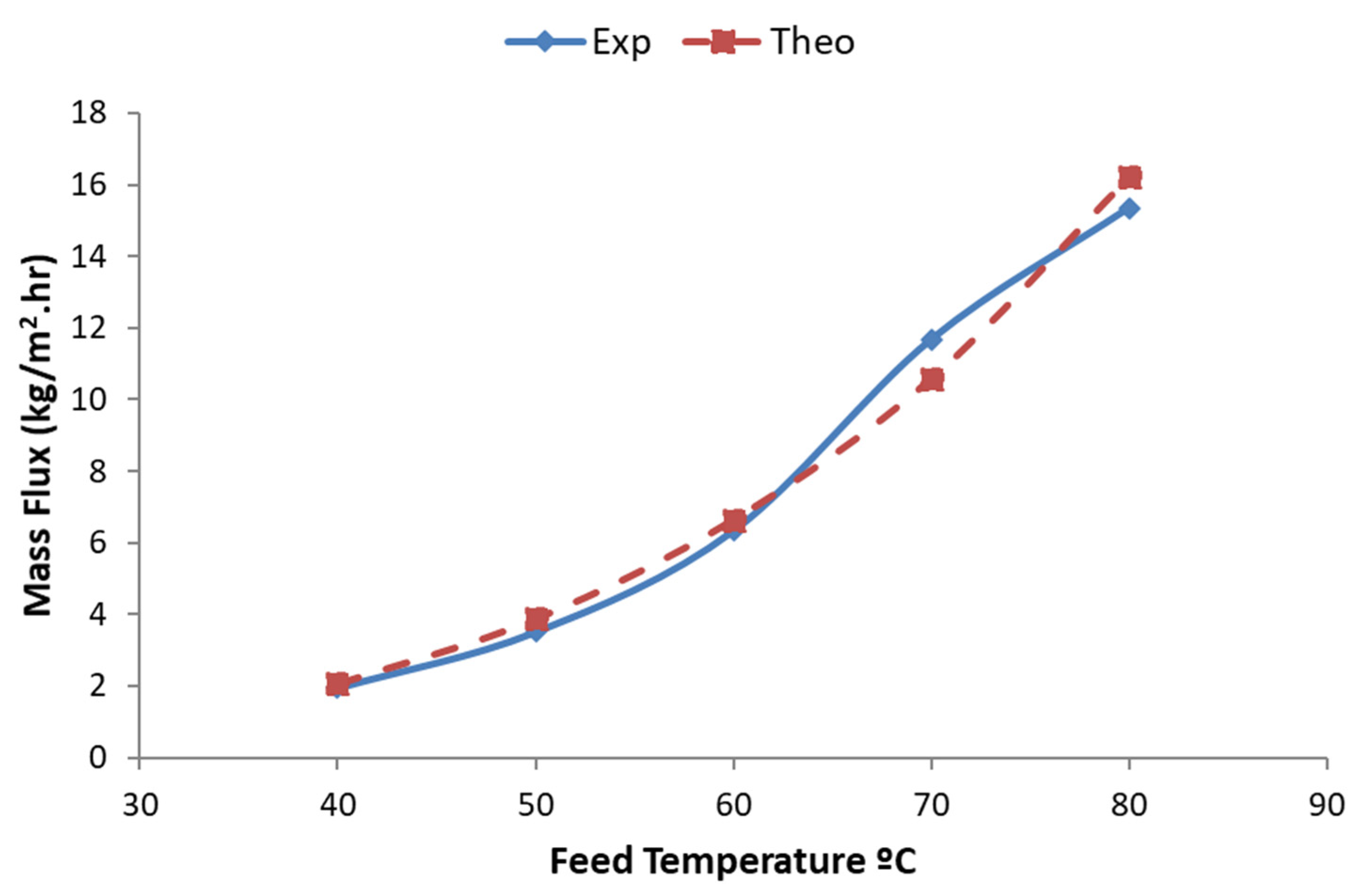
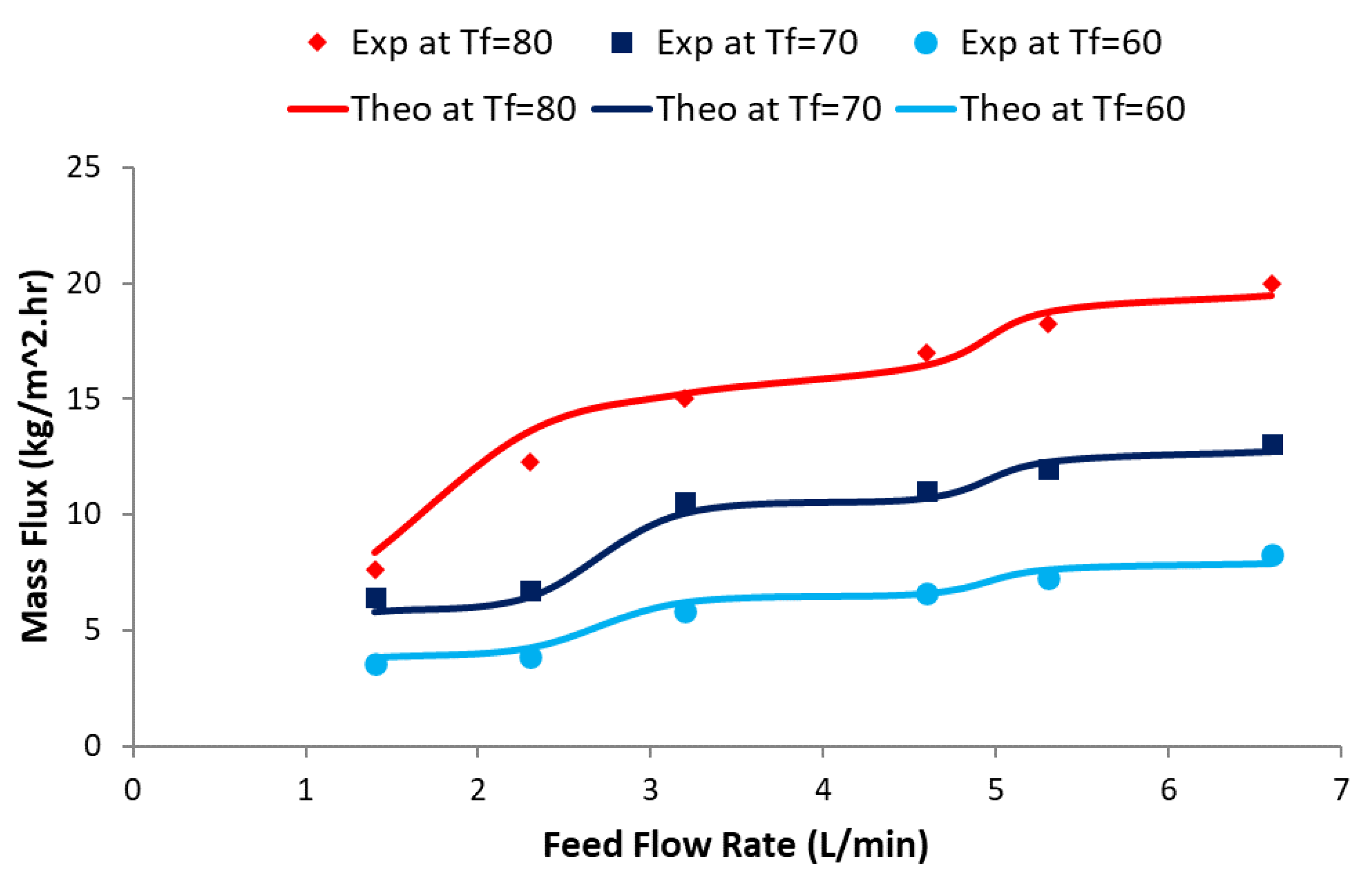
4. Results and Discussion

In this section, the results from experiments and the theoretical model are presented and discussed. The purpose of these experiments is to look at the effect of feed water temperature and salinity on the permeate mass flux and the maximum possible recovery ratio. Initial experiments were conducted with feed water salinities of 10,000 ppm (1%) and 30,000 ppm (3%). The main purpose of these tests was to establish base care mass flux results with low salinity that provides the upper limit for mass flux. Figure 6 shows the effect of permeate temperature on the performance of DCMD. In this study, the permeate temperature varied between 5 °C to 20 °C; at different feed temperatures, the feed salinity was kept constant at 10,000 ppm (1% wt.%) and the feed and permeate flow rates were also kept constant at 4 L/min. Decreasing the permeate water temperature results in increasing the mass flux; this is due to the increase of temperature difference across the membrane surface, which results in significant transmembrane vapor pressure difference and hence causes an increase in mass flux.

In order to improve the performance of DCMD, one can either increase the feed temperature or decrease the permeate temperature. However, the increase in mass flux is more profound when increasing the feed temperature than when decreasing the permeate temperature. For instance, at T_f = 80 °C, when the permeate temperature dropped from 20 °C to 10 °C, the mass flux increased by nearly 2.9%; on the other hand, at T_p = 10 °C, when the feed temperature increased from 70 °C to 80 °C, the mass flux increased by nearly 52%. During the experiments, the mass flow rate was measured with a digital scale and a digital timer; uncertainty due to instrumental and measurement accuracies was estimated to be around ±6% (following the law of error propagation).

The second set of initial experiments was conducted with feed at close to sea water salinity of around 30,000 ppm (3% wt.), and the feed water temperature was varied from 40 °C to 80 °C, while the permeate was maintained at 15 °C. The feed and permeate flow rates were maintained constant at 4.6 L/min. Figure 7 illustrates the relationship of mass flux and feed temperature. Due to the increase of vapor pressure with temperature, mass flux is observed to increase significantly with increasing temperature; this is due to the increased temperature difference between the feed and permeate sides. This increases the vapor pressure difference across the membrane and hence the driving force of the movement of water vapor molecules through the membrane. Here, the starting salinity of the feed was low, and the duration of the experiments was very short, hence there was no significant increase in the feed water salinity during each experiment that could affect the mass flux. Further, it can be seen that the increase in salinity from 10,000 ppm (1% wt.) to 30,000 ppm (3% wt.) does not have any visible influence on the mass flux. The main reason for this is that at 1% or 3%, the salinity polarisation on the feed side is not very predominant to cause visible change in the flux. However, the temperature of the feed has visible effect on the flux, as the driving force significantly increases at higher temperature differences and there is slight decrease in the latent heat of vaporisation at higher temperatures.

To study the effect of flow rate, experiments are done at a constant permeate temperature of 15 °C, three different feed temperatures of 60 °C, 70 °C and 80 °C and at a constant feed salinity of 30,000 ppm. From Figure 8 it is shown that the mass flux increases as the flow rate increases. The module has a channel width of 128 mm and a channel height of 2 mm; this provides a cross-sectional area of 256 mm². With the range of feed flow rate between 1.4 L/min to 6.6 L/min, the average flow velocity varies from 0.1 m/s to 0.4 m/s. With this velocity, the Reynolds number ranges from 400 to 1900, which means the flow regime is laminar. The addition of the supporting mesh helps create local turbulence, and the effect of the average flow velocity is not very apparent on the mass flux. The increase of flow rate results in an increase of localized turbulence, which results in an enhancement in heat and mass transfer in both the feed and permeate sides of the membrane, since this will reduce the thermal boundary layer and hence drop the temperature and salinity polarization effects. Besides, it improves the heat transfer through the membrane because the heat loss due to conduction per unit trans-membrane flux decreases. The mass flux can either be improved by increasing the feed temperature, increasing the mass flow rate or both. However, the increase of flow rate comes at a cost of higher pumping power. Consequently, an optimization should be done to choose the suitable and most appropriate working conditions.

To investigate the desalination of high saline water, another set of experiments was started with 10 kg of feed water with 30,000 ppm TDS and 5 kg of permeate with 70 ppm TDS. The experiments involved extended testing that allowed the feedwater volume to decrease and the permeate water volume to increase over time. Feed water salinity increased over time, and permeate water salinity decreased, which proves the transport of water vapor from the feed side to the permeate side and the production of fresh water. The permeate water salinity was recoded to ensure that no leakage or membrane wetting happened during the experiment. Figure 9 presents the change of feed and permeate water salinities over time. During this experiment, the effect of increased salinity on the mass flux was also monitored while keeping temperature and flow rate of feed water and permeate constant. The effect of feed salinity is presented in Figure 10. The experiments were done at the same feed and permeate temperature, 70 °C and 20 °C, respectively, and a feed and permeate flow rate of 3 L/min. It is observed that the mass flux decreases with increasing feed water salinity. The reduction in mass flux as the feed salinity increases is due to the rising effect of the salt concentration polarization that enhances the resistance for flow of the vapor to the permeate side across the membrane. Besides that, the partial vapor pressure of water also decreases with increasing feed salinity and hence causes the driving force of DCMD to reduce. To compensate for the decrease in the mass flux due to the rise in salinity, a larger membrane area should be considered when designing zero liquid discharge systems based on MD. It can be seen that a 10-fold increase in the salinity causes a 5-fold decrease in the mass flow, so, as a rule of thumb, the membrane area can be doubled for practical applications.

Figure 11 presents results from the experiments that were conducted at a three constant feed water temperature of 85 °C, 75 °C and 65 °C and an average permeate temperature of 30 °C. Both the feed water and permeate water flow rates were kept constant at 3 L/min. As the salinity increased, the mass flux decreased due to the increase of resistance of vapor flow transfer caused by the effect of concentration polarization at the surface of the membrane. The mass flux kept reducing to almost zero as the feed water salinity approached around 300,000 ppm TDS, which is very close to supersaturation. At feed water salinity of around 282,000 ppm TDS, small salt crystals started to form on the water surface in the feed water tank, as shown in Figure 12.

To assess the quality of the produced fresh water and the effectiveness of DCMD, the salt rejection factor (SRF) values were calculated using Equation (26), and, as can be seen in Figure 13 initially, the SRF was 99.78%, then, as the feed salinity increased to 308,092 ppm, the SRF increased as well, reaching 99.99%. These results prove the competence of DCMD to operate efficiently at high salinities up to crystallization.

$$SRF=\frac{Feed concentration-Permeate conncentration}{Feed concentration}\times 100$$

(26)

Initially, the experiment commenced at 10 L feed water with 30,000 ppm TDS and was run up to crystallization where the feed water salinity reached 308,092 ppm TDS, which is very close to supersaturation. The total amount of produced freshwater is 8.01 L, which indicates that the recovery rate is around 80%. It is noteworthy that the final volume of feedwater was 1 L, which implies that some water vapor has been lost during the experiment despite the fact that the urn was covered to recover any water vapor.

5. Conclusions

A detailed experimental set up of the DCMD system is presented. Thorough experimental findings on the performance of DCMD are provided. The effects of operating conditions on DCMD are studied, and high mass flux values were achieved at high feed temperatures, low permeate temperatures, high flow rates and low feed salinities. A theoretical model was also developed to validate the experimental results, and from the previous graphs, it can be seen that the theoretical model is in good agreement with the experimental results; this model was used to calculate the mass flux. This model can be used in the future to design a new module for specific working conditions (in combination with solar energy) and predict the performance of the system. The possibility of desalinating high salinities water is investigated. DCMD proved its effectiveness to produce high quality freshwater at salinities close to 290,000 ppm, which can lead to Zero Liquid Discharge desalination.

References

1. Khayyam, H.; Naebe, M.; Milani, A.S.; Fakhrhoseini, S.M.; Date, A.; Shabani, B.; Atkiss, S.; Ramakrishna, S.; Fox, B.; Jazar, R.N. Improving energy efficiency of carbon fiber manufacturing through waste heat recovery: A circular economy approach with machine learning. Energy 2021, 225, 120113. [Google Scholar] [CrossRef]
2. Phan, D.; Moradi Amani, A.; Mola, M.; Asgharian Rezaei, A.A.; Fayyazi, M.; Jalili, M.; Pham, D.; Langari, R.; Khayyam, H. Cascade Adaptive MPC with Type 2 Fuzzy System for Safety and Energy Management in Autonomous Vehicles: A Sustainable Approach for Future of Transportation. Sustainability 2021, 13, 10113. [Google Scholar] [CrossRef]
3. Khayyam, H. Automation, Control and Energy Efficiency in Complex Systems; MDPI Books: Basel, Switzerland, 2020. [Google Scholar]
4. Voutchkov, N. Desalination–Past, Present and Future; International Water Association: London, UK, 2016. [Google Scholar]
5. Kalogirou, S.A. Seawater desalination using renewable energy sources. Prog. Energy Combust. Sci. 2005, 31, 242–281. [Google Scholar] [CrossRef]
6. Qtaishat, M.R.; Banat, F. Desalination by solar powered membrane distillation systems. Desalination 2013, 308, 186–197. [Google Scholar] [CrossRef]
7. Sadhwani, J.J.; Veza, J.M.; Santana, C. Case studies on environmental impact of seawater desalination. Desalination 2005, 185, 1–8. [Google Scholar] [CrossRef]
8. Al-Mutaz, I.S. Environmental impact of seawater desalination plants. Environ. Monit. Assess. 1991, 16, 75–84. [Google Scholar] [CrossRef] [PubMed]
9. Lawson, K.W.; Lloyd, D.R. Membrane distillation. J. Membr. Sci. 1997, 124, 1–25. [Google Scholar] [CrossRef]
10. Curcio, E.; Drioli, E. Membrane distillation and related operations—A review. Sep. Purif. Rev. 2005, 34, 35–86. [Google Scholar] [CrossRef]
11. Cath, T.Y.; Adams, V.D.; Childress, A.E. Experimental study of desalination using direct contact membrane distillation: A new approach to flux enhancement. J. Membr. Sci. 2004, 228, 5–16. [Google Scholar] [CrossRef]
12. Martinetti, C.R.; Childress, A.E.; Cath, T.Y. High recovery of concentrated RO brines using forward osmosis and membrane distillation. J. Membr. Sci. 2009, 331, 31–39. [Google Scholar] [CrossRef]
13. Khayet, M.; Matsuura, T. Chapter 1—Introduction to Membrane Distillation. In Membrane Distillation; Khayet, M., Matsuura, T., Eds.; Elsevier: Amsterdam, The Netherlands, 2011; pp. 1–16. [Google Scholar]
14. Nakoa, K.; Rahaoui, K.; Date, A.; Akbarzadeh, A. An experimental review on coupling of solar pond with membrane distillation. Sol. Energy 2015, 119, 319–331. [Google Scholar] [CrossRef]
15. Nakoa, K. Sustainable zero liquid discharge desalination. Sol. Energy 2016, 135, 337–347. [Google Scholar] [CrossRef]
16. Rahaoui, K.; Ding, L.C.; Tan, L.P.; Mediouri, W.; Mahmoudi, F.; Nakoa, K.; Akbarzadeh, A. Sustainable membrane distillation coupled with solar pond. Energy Procedia 2017, 110, 414–419. [Google Scholar] [CrossRef]
17. Camacho, L.M.; Dumée, L.; Zhang, J.; Li, J.-d.; Duke, M.; Gomez, J.; Gray, S. Advances in membrane distillation for water desalination and purification applications. Water 2013, 5, 94–196. [Google Scholar] [CrossRef] [Green Version]
18. Alklaibi, A.M.; Lior, N. Membrane-distillation desalination: Status and potential. Desalination 2005, 171, 111–131. [Google Scholar] [CrossRef]
19. Alkhudhiri, A.; Darwish, N.; Hilal, N. Membrane distillation: A comprehensive review. Desalination 2012, 287, 2–18. [Google Scholar] [CrossRef]
20. Banat, F.; Jwaied, N.; Rommel, M.; Koschikowski, J.; Wieghaus, M. Performance evaluation of the “large SMADES” autonomous desalination solar-driven membrane distillation plant in Aqaba, Jordan. Desalination 2007, 217, 17–28. [Google Scholar] [CrossRef]
21. El-Abbassi, A.; Hafidi, A.; Khayet, M.; García-Payo, M.C. Integrated direct contact membrane distillation for olive mill wastewater treatment. Desalination 2013, 323, 31–38. [Google Scholar] [CrossRef]
22. Goh, S.; Zhang, J.; Liu, Y.; Fane, A.G. Fouling and wetting in membrane distillation (MD) and MD-bioreactor (MDBR) for wastewater reclamation. Desalination 2013, 323, 39–47. [Google Scholar] [CrossRef]
23. Banat, F.; Jwaied, N.; Rommel, M.; Koschikowski, J.; Wieghaus, M. Desalination by a “compact SMADES” autonomous solarpowered membrane distillation unit. Desalination 2007, 217, 29–37. [Google Scholar] [CrossRef]
24. Alves, V.D.; Coelhoso, I.M. Orange juice concentration by osmotic evaporation and membrane distillation: A comparative study. J. Food Eng. 2006, 74, 125–133. [Google Scholar] [CrossRef]
25. Gunko, S.; Verbych, S.; Bryk, M.; Hilal, N. Concentration of apple juice using direct contact membrane distillation. Desalination 2006, 190, 117–124. [Google Scholar] [CrossRef]
26. Godino, M.P.; Peña, L.; Rincón, C.; Mengual, J.I. Water production from brines by membrane distillation. Desalination 1997, 108, 91–97. [Google Scholar] [CrossRef]
27. Phattaranawik, J.; Jiraratananon, R.; Fane, A. Effect of pore size distribution and air flux on mass transport in direct contact membrane distillation. J. Membr. Sci. 2003, 215, 75–85. [Google Scholar] [CrossRef]
28. Khayet, M. Membranes and theoretical modeling of membrane distillation: A review. Adv. Colloid Interface Sci. 2011, 164, 56–88. [Google Scholar] [CrossRef]
29. Qtaishat, M.; Matsuura, T.; Kruczek, B.; Khayet, M. Heat and mass transfer analysis in direct contact membrane distillation. Desalination 2008, 219, 272–292. [Google Scholar] [CrossRef]
30. Schofield, R.; Fane, A.; Fell, C. Heat and mass transfer in membrane distillation. J. Membr. Sci. 1987, 33, 299–313. [Google Scholar] [CrossRef]
31. Srisurichan, S.; Jiraratananon, R.; Fane, A. Mass transfer mechanisms and transport resistances in direct contact membrane distillation process. J. Membr. Sci. 2006, 277, 186–194. [Google Scholar] [CrossRef]
32. Martínez-Díez, L.; Vazquez-Gonzalez, M.I. Temperature and concentration polarization in membrane distillation of aqueous salt solutions. J. Membr. Sci. 1999, 156, 265–273. [Google Scholar] [CrossRef]
33. Khalifa, A.; Ahmad, H.; Antar, M.; Laoui, T.; Khayet, M. Experimental and theoretical investigations on water desalination using direct contact membrane distillation. Desalination 2017, 404, 22–34. [Google Scholar] [CrossRef]
34. Hawlader, M.N.A.; Bahar, R.; Ng, K.C.; Stanley, L.J.W. Transport analysis of an air gap membrane distillation (AGMD) process. Desalination Water Treat. 2012, 42, 333–346. [Google Scholar] [CrossRef]
35. Lawson, K.W.; Lloyd, D.R. Membrane distillation. II. Direct contact MD. J. Membr. Sci. 1996, 120, 123–133. [Google Scholar] [CrossRef]
Figure 1. DCMD configuration.
Sustainability 13 10860 g001
Figure 2. Heat and mass transfer in DCMD.
Sustainability 13 10860 g002
Figure 3. Algorithm for heat and mass transfer.
Sustainability 13 10860 g003
Figure 4. Components and assembly of DCMD module: (a) PTFE membrane; (b) mesh; (c) gasket; (d) acrylic frame; (e) DCMD module assembly.
Sustainability 13 10860 g004
Figure 5. (a) Schematic of the membrane distillation system; (b) experimental setup design.
Sustainability 13 10860 g005
Figure 6. Experimental and theoretical results. Effect of permeate temperature on mass flux at different feed temperatures.
Sustainability 13 10860 g006
Figure 7. Effect of feed temperature on mass flux. Comparison of theory and experiments.
Sustainability 13 10860 g007
Figure 8. Experimental and theoretical results. Effect of flow rates of feed and permeate on mass flux at different feed temperatures.
Sustainability 13 10860 g008
Figure 9. Change of the feed and permeate salinities over time.
Sustainability 13 10860 g009
Figure 10. Experimental and theoretical results. Effect of feed salinity on mass flux.
Sustainability 13 10860 g010
Figure 11. Change of mass flux with the feed water salinities.
Sustainability 13 10860 g011
Figure 12. (a) initial thin salt crystal formation at around 282,000 ppm; (b) larger crystals and heavy precipitation when the feed water salinity reached 308,00 ppm.
Sustainability 13 10860 g012
Figure 13. Change of salt rejection factor with the change of feed salinity.
Sustainability 13 10860 g013
Publisher’s Note: MDPI stays neutral with regard to jurisdictional claims in published maps and institutional affiliations.