
Multi-Objective Optimization for Healthcare Waste Management Network Design with Sustainability Perspective


1
Faculty of Engineering and Natural Sciences, Sabanci University, Istanbul 34956, Turkey
2
Department of Maritime and Logistics Management, Australian Maritime College, University of Tasmania, Launceston, TAS 7248, Australia
3
Department of Industrial Engineering, Istinye University, Istanbul 34010, Turkey
*
Author to whom correspondence should be addressed.
Sustainability 2021, 13(15), 8279; https://doi.org/10.3390/su13158279
Submission received: 27 May 2021
/
Revised: 7 July 2021
/
Accepted: 20 July 2021
/
Published: 24 July 2021
(This article belongs to the Special Issue Sustainable Global Supply Chain Management: From an International Perspective)
Abstract
:Healthcare Waste Management (HWM) is considered as one of the important urban decision-making problems due to its potential environmental, economic, and social risks and damages. The network of the HWM system involves important decisions such as facility locating, inventory management, and transportation management. Moreover, with growing concerns towards sustainable development objectives, HWM systems should address its environmental and social aspects as well as its economic and technical characteristics. In this regard, this paper formulates a novel multi-objective optimization model to empower companies in making optimized decisions considering the economic, environmental, and social aspects. Within the proposed model, the first objective function aims to minimize the transportation costs, processing costs, and establishment costs. The second objective function aims to minimize environmental risks and emissions related to the transportation of waste between facilities. The third objective function aims to maximize job creation opportunities. Formulating these three functions, an Improved Multi-Choice Goal Programing (IMCGP) approach is proposed to solve the multi-objective optimization model, which is then compared with the Goal Attainment Method (GAM). Finally, to show the applicability and feasibility of the proposed model, an illustrative example of healthcare waste management is analyzed, and the results are discussed.
1. Introduction
In the last decade, there have been increasing pressures from different stakeholders such as end-consumers and government agencies demanding more attention towards the concept of sustainable development [1]. Today, organizations are no longer consider themselves as isolated entities as they are facing a wider network which motivates them to collaborate with different players in such a complex network to create a sustainable business environment [2,3]. Particularly, since the introduction of the concepts of sustainable development and the circular economy, cities have made attempts to restructure their important infrastructures such as waste management systems to be aligned with the guidelines and principles of the sustainability framework [4,5]. One of the main environmental sustainability issues in urban communities and municipalities is associated with a high generation rate of healthcare waste (HW) from hospitals and medical centers [6,7]. The HW rate has increased exponentially due to several factors such as population growth, high demand for healthcare services, and the high consumption rate of materials in medical centers [8]. This issue is critically important, as generating more environmental hazards can significantly endanger public health. Previous works have highlighted the potential problems caused by ineffective methods of waste disposal [9].
Considering the dangerous negative effects of the inappropriate HW treatment on humans’ life including environmental, economic, and social issues, highly populated cities are seeking to develop a reliable HW management (HWM) system for the optimal planning of collection, processing, recycling, disposal, and transportation of waste [10,11]. One of the main solutions that municipalities are applying is related to the establishment of waste collection stations and waste sorting centers. This can provide efficient low-pollution services through recycling usable wastes and delivering waste to suitable waste treatment facilities [12]. HW is mainly associated with a high proportion of plastic waste and metal waste, which is included in every medical material. Due to the recyclable nature of these elements, recycling HW would ultimately create many economic, environmental, and social advantages for cities, medical centers, and waste organizations. For example, recycled HW can be reutilized through secondary markets, which would act as delivery points between HWM systems and consumers. Despite the significance of this issue, there is a lack of research on developing a comprehensive framework that considers sustainability issues in dealing with HW disposal. In addition, HWM systems are highly complex systems with many players involved in their network, which makes the optimal planning of the HWM network more beneficial for the related stakeholders. The purpose of this study is to provide an optimal and sustainable planning framework for HWM through minimizing the total cost of the system (establishment cost, operational cost, transportation cost) and its environmental pollutants as well as maximizing the attention paid to the social concerns of urban communities (job creation opportunities). In detail, this study aims to tackle sustainable HWM network design to efficiently deal with HW collection from hospitals and medical centers, transportation through the network, transferring recyclable HW from waste sorting centers to recycling centers, and finally, to secondary markets where the final consumer would receive it.
The rest of the paper is organized as follows. Section 2 presents a comprehensive literature review related to previous work in the field of waste management. Section 3 includes the problem definition, notations, and mathematical models. Section 4 presents an illustrative example, the results, and a discussion. Finally, we conclude in Section 5.
2. Literature Review
This section presents an in-depth literature review of location problems, vehicle routing problems, and network design problems for the HWM network.
Due to the high complexity of problems associated with HWM, previous studies have applied various approaches to address specific problems. Mathematical models are among the frequently applied methods to tackle the facility location problems (FLP), vehicle routing problems (VRP), network design problems (NDP), inventory management problems (IMP), and allocation problems within HWM systems [13]. Mathematical modeling has several advantages in comparison to other methods such as simulation modeling or soft computing-based models. First, mathematical modeling enables us to simply and precisely model a real-life situation with many constraints. In other words, mathematical modeling allows us to accurately represent a reality into a mathematical model. Due to its fundamentals, mathematical modelling can give us a better understanding of the different situations in real-life based on the nature of decision variables. In better words, we can state that mathematical modeling empowers decision makers to understand insights and information based on formulation of a problem. Due to the complexity and big data nature of decision-making problems, mathematical modeling is an efficient tool which saves time, effort, and money. Meanwhile, other related problems such as socioeconomic analysis and technology selection for HWM systems have been addressed by using multi-criteria decision-making [14,15] and machine learning [16] techniques.
In one of the first studies in the field of HWM, Beltrami and Bodin [17] used VRP to address the waste collection of municipalities of New York and Washington with respect to different characteristics of transportation modes. Later, Kim et al. [18] formulated a mathematical model to address multi-trip VRP with time windows for municipal waste collection with an aim to minimize the number of vehicles and total travel time to satisfy all demands. In a similar study, Buhrkal et al. [19] used VRP with time windows for efficient waste collection modes and transportation vehicles with minimum traveling cost. Huang and Lin [20] characterized the waste collection problem as a set-covering problem and VRP problem with inter-arrival time constraints to minimize the number of vehicles and distance traveled. Heuristic algorithms were applied to tackle the model for a numerical example. Louati [21] proposed a multi-objective VRP considering several transfer stations, collection sites, and different transportation vehicles. Asefi et al. [22] proposed a bi-objective mathematical model for VRP considering the fleet size to minimize transportation costs in waste management systems as well as to minimize the total deviation from the right load allocation to waste transfer stations. Wu et al. [23] formulated a chance-constrained-based VRP for wet waste collection to minimize costs and emissions. Particle swarm optimization and simulated annealing algorithms were applied to solve the proposed model. Ghannadpour et al. [24] proposed a multi-objective optimization model for VRP to address healthcare waste collection from small medical centers with a focus on minimizing economic and environmental concerns and social health risks.
To further tackle the complexity of HWM networks, the location-routing problem (LRP), as an extension of the classical routing problem combining VRP and FLP, has been studied as one of the useful methods to address strategic and operational decisions in the HWM network. In one of the very first studies in HWM network design, Zografros and Samara [25] suggested LRP as a promising framework for addressing the transportation and disposal of hazardous material through minimizing disposal risks and travel time. Alumur and Kara [26] proposed a modified formulation for LRP to both minimize the total cost of the system and transportation risk for the HWM of Turkey. Shi et al. [27] developed a MILP model to minimize the overall logistics costs of the reverse network of medical waste using the genetic algorithm. Das et al. [28] formulated a multi-objective optimization model for LRP to minimize the costs and transportation risks. Mohsenizadeh et al. [29] proposed a bi-objective MILP model for waste management network design with a focus on minimizing the total cost of the system and greenhouse gas emissions through locational planning and routing problems. Darmian et al. [30] formulated a multi-objective location-based mathematical model to determine optimal locations for solid waste management considering economic, environmental, and social factors using a heuristic algorithm. Kargar et al. [11] studied the reverse logistics network of HWM during the COVID-19 pandemic. They formulated multi-objective linear programming to minimize the total costs, transportation risks, and HW treatment. Yu et al. [10] suggested multi-objective programming to address a multi-period reverse logistics of waste management systems during the COVID-19 era.
Recently, Tirkolaee et al. [31] proposed a multi-objective MILP model for a multi-trip location-routing problem with time windows for HWM considering sustainability factors during the COVID-19 pandemic. To address the possible uncertainty within the parameters of the model, they formulated their model under fuzzy chance-constrained programming. Zaeimi and Rassafi [32] formulated a multi-objective MILP under fuzzy chance-constrained programming to minimize the total costs of the network as well as environmental emissions under uncertain information.
Table 1 summarizes the goals of the current study and the recent important studies in the literature of sustainable waste management.
According to the above survey, it should be mentioned that a multi-objective mathematical model is developed in this study in order to optimally plan the HWM network with a sustainability perspective. In the formulated MILP, the objectives aim to minimize the total cost of the HWM system, minimize environmental pollutions, and maximize social factors such as job creation opportunities within the established facilities. To sum up, the contributions of this study are (i) the formulation of a multi-objective mathematical model for sustainable healthcare waste management, (ii) the network design of healthcare waste management considering treatment, disposal, and recycling facilities, (iii) the consideration of sustainability factors such as cost, environmental and emission risks, and job creation, and (iv) the investigation of an illustrative example for the proposed optimization model.
3. Problem Definition
This section describes the problem and the proposed mathematical model according to the main assumptions. Consider a sustainable HWM system including waste generation centers, waste treatment centers, waste recycling centers, and waste disposal centers (see Figure 1). The aim is to find the optimal policy in terms of the best locational decisions, allocation, and transportation planning within the network. Due to this, a set of assumptions is first defined based on the real-world conditions to formulate the problem which is given as follows:
- (1)
- Locational decisions are made on the levels of treatment, recycling, and disposal centers;
- (2)
- Three types of vehicles are defined to be used between different levels, where the first type of transportation vehicles are used between waste generation centers and waste treatment centers/waste recycling centers, the second type of transportation vehicles are used between the waste treatment centers and the waste recycling centers/waste disposal centers, and the third type of transportation vehicles are used between the waste recycling centers and waste disposal centers;
- (3)
- A planning horizon is considered;
- (4)
- There are multiple types of HW;
- (5)
- All the parameters are deterministic;
- (6)
- Waste generation points include hospitals and infirmaries;
- (7)
- The given flow rates of waste are regarded between different centers;
- (8)
- The capacity of different centers is limited as well as the capacity of the vehicles.
To address the sustainability of the system, three objective functions of total cost minimization, total population risk minimization, and the total number of job opportunities are followed in the problem.
The proposed multi-objective MILP model is given in the following subsection.
Mathematical Model
The proposed mathematical model is defined as follows:
- 1.
- Objective Functions
Equation (1) represents the first objective function of the model, which seeks to minimize the total cost. The first 5 terms stand for the transportation costs, terms 6–8 represent the processing costs, terms 9–11 show the establishment costs, and terms 12–14 display the usage costs of vehicles,
Equation (2) represents the second objective function, which tries to minimize the total population risk for transporting waste between different facilities.
Equation (3) represents the third objective function, which maximizes the total number of job opportunities after establishing the treatment, recycling, and disposal centers. According to Equations (1)–(3), three pillars of sustainable development are defined.
- 2.
- Constraints
Constraints (4)–(6) indicate the capacity limitation of treatment, recycling, and disposal centers, respectively.
Constraints (7) and (8) express the capacity limitation of the first type of vehicles.
Constraint (9) and (10) state the capacity limitation of second type of vehicles.
Constraint (11) denotes the capacity limitation of third type of vehicles.
Constraint (12) ensures that a specific amount of demand should be transferred to treatment centers.
Constraint (13) guarantees that the remaining amount of demand is transferred to recycling centers.
Constraints (14) and (15) control the output flows of waste from treatment centers towards recycling and disposal centers, respectively.
Constraint (16) calculates the amount of output flows from recycling centers towards disposal centers.
Constraint (17) displays the types of variables.
4. Improved Multi-Choice Goal Programming (IMCGP)
IMCGP was first presented by Jadidi et al. [44] as an improved variant of the goal programming (GP) approach. It is one of the recently extended versions of GP that has attracted much attention from researchers [45,46]. The main advantages of IMCGP are summarized as follows. It adds a priority function and considers a goal interval instead of a single goal. The main motivation is that since, in some cases, the objective function value may violate the expected or desire level, a penalty should be taken into account in the model. This feature has not been studied by previous variants of GP techniques [35]. Accordingly, due to the high probability of an unforeseen amount of waste in medical centers, the IMCGP method is utilized to tackle our proposed multi-objective model.
Based on the IMCGP method and to provide a final single-objective MILP model, Equation (18) is introduced as the new objective function of the problem. Moreover, Equations (19)–(24) are incorporated into the model as the new constraints while keeping Equations (4)–(17).
subject to.
where represents a positive continuous variable (coefficient)—the normalized distance of jth objective functions from which takes a value between 0 and 1. Moreover, and stand for the desirable and undesirable values of jth objective function. Here, represents the aspiration interval of jth objective functions to be determined by the decision maker. In this study, the upper bound of the aspiration interval () is assumed to be equal to , while the lower bound of the aspiration interval () takes a value greater than or equal to . In other words, the interval is broken down into the more desirable interval and the less desirable one . Furthermore, shows the normalized distance of the jth objective function from . If the value of the jth objective function is greater than , then a penalty is regarded, which takes a value between 0 and 1. Finally, is defined as a binary variable, and and denote the weight of the jth objective function with respect to and .
Equations (4)–(17),
5. Illustrative Example
In this section, a numerical example is illustrated to test the applicability of the proposed methodology. To this end, CPLEX solver/GAMS software is employed to run the final model within a time limitation of 3600 s. The information related to the examples and the values of the parameters is given in Table 2 and Table 3. It should be noted that these required data are adapted from similar research studies in the literature, such as Tirkolaee et al. [38].
Table 2 represents information about every index that is used in the proposed mathematical model. In this regard, 20 waste generation centers are considered, which are supposed to be allocated to 6 waste treatment centers, 6 waste recycling centers, and 6 disposal centers.
Now, the computational results are reported in Table 4 in terms of objective function values and runtime.
According to the results obtained, all the vehicles of different types are used in each time period to optimize the problem. Moreover, the numbers of the established treatment, recycling and disposal centers are six, four, and two, respectively. Therefore, the proposed model aims to optimally allocate the suitable waste types to the treatment and recycling centers rather than to the disposal centers. Therefore, in real-life practices, this can ensure that the municipalities can financially maximize their profit through treatment and recycling centers. Along with the objective function value for economic and environmental aspects, Z3 represents how many jobs can be created by designing an appropriate and comprehensive network to address healthcare waste. Therefore, for the small illustrative example, the results indicate that 1684 job opportunities can be created, which is for sure a noticeable number in terms of both social and economic aspects. Therefore, for real-life practices with large-scale datasets, the results denote that a high number of job opportunities can be created which can definitely affect the unemployment rate in every city. On the other hand, the proposed mathematical model aims to denote the waste collection and treatment problem with a network analysis where the decision maker can optimize the transferring task of waste based on their type, generation center, and treatment center with the most suitable transportation vehicles. This would not only bring up economic impacts for urban waste management systems, but it would also define the safest transfer operations in order to decrease profit loss and environmental issues. Locating waste management centers is one of the challenging problems that managers always deal with in this sector. The model empowers real-life decision makers and managers in healthcare waste management systems to make a decision on establishing treatment, recycling, and disposal centers in the most suitable locations in order to both increase the economic advantages and to minimize the environmental risks. As healthcare and medical waste types are very different from municipal solid waste, transportation operations with suitable vehicles are of high significance for the organization. In this regard, our results show how the optimized selection of vehicle types can be beneficial for the whole network. As can be seen, the proposed methodology could find the optimal solution within just 5.27 s, which highlights a high efficiency. In the following section, a set of sensitivity analyses is carried out to evaluate the behavior of the objective functions against the changes of key parameters. However, the model includes important parameters such as the capacity for different facilities as well as the flow rate, which can have dramatic effects on the computational running time and complexity of the model if we consider possible restrictions or uncertainty for them. As the waste generation rate is very sensitive to different events in our daily life, there is inevitable uncertainty whether we will observe any sudden decrease or increase in its rate due to unexpected events such as the COVID-19 pandemic. Thus, waste generation rate is also another crucial parameter that can have serious impacts on the computational time and complexity if the uncertainty is regarded.
5.1. IMCGP vs. GAM
Here, the performance of the proposed IMCGP is evaluated against one of the most applicable and well-known multi-objective decision-making (MODM) techniques, i.e., the Goal Attainment Method (GAM). The GAM was introduced by Gebicki [47]. It contains a set of ideal goals, , which are concerned with a set of objective functions, . The ideal goal of each objective function is obtained by optimizing the single-objective model using that objective function. Moreover, a set of weights (importance degrees) are assigned to each objective function where . Now, the GAM formulation corresponding to our proposed model is given as follows:
subject to
Equations (4)–(17).
Here, we consider () = (0.5, 0.3, 0.2) as well as the values taken into account by IMCGP. Now, the comparison results are given in Table 5.
As can be seen in Table 5, different outputs are obtained for IMCGP and GAM. Accordingly, GAM could just outperform IMCGP in terms of while it requires a runtime that is approximately 24.56 times larger than IMCGP. It is demonstrated that IMCGP is the superior solution method.
5.2. Sensitivity Analysis
Here, a set of sensitivity analyses are performed on the key parameters of (amount of waste type generated at waste generation center in period ), (flow rate of generated waste type which is transferred from waste generation center to waste treatment centers in period ), (flow rate of generated waste type which is transferred from waste treatment center to waste recycling centers in period ), and (flow rate of generated waste type which is transferred from waste recycling center to waste disposal centers in period ). Accordingly, the change intervals of −20%, −10%, 0%, +10%, and +20% are taken into account to assess the behavior of the objective functions. The obtained results are represented in Table 6 (“-” denotes an infeasible solution).
As can be seen from Table 5 and Figure 2, different behaviors are observed from the objective functions over the given change intervals. It means that the instability of real-world can directly affect the problem and change the optimal policy. For example, any changes in the key parameters decrease and the maximum (optimal) value of this objective function is achieved just at the change interval of 0%. This condition exactly occurs for where the maximum (optimal) value is attained at the change interval of 0%. On the other hand, the problem turned out to be infeasible over some change intervals. For example, there is no feasible region to find the optimal solution for the 20% increase in and . This means that the managers and decision makers should examine the number of available resources in the system.
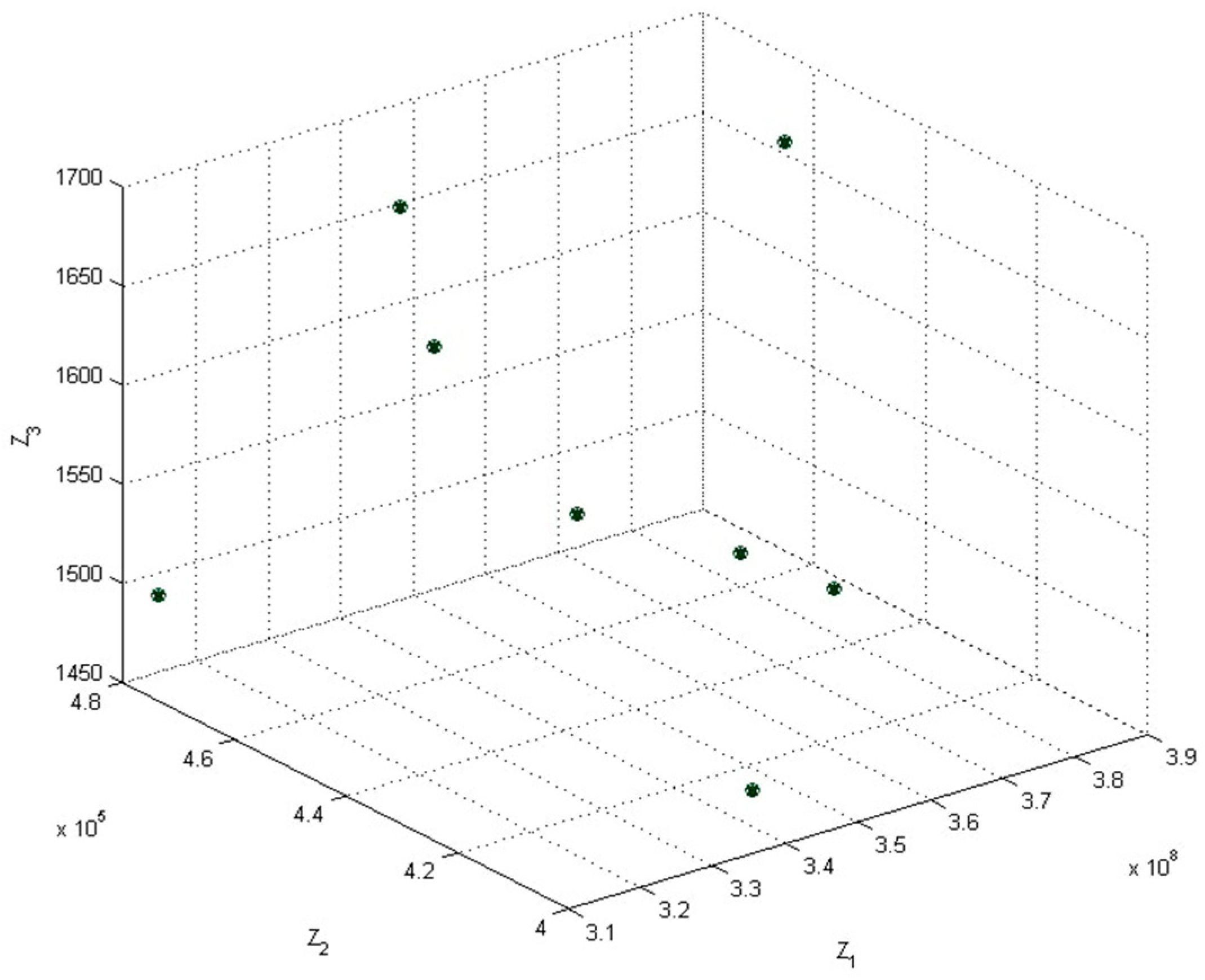
On the other hand, eight different combinations of and are taken into account to study the behavior of the objective functions, such as a Pareto front. The obtained results are outlined in Table 7 and Figure 3.
According to Figure 3, the decision maker can choose the most suitable point as the optimum in order to analyze and implement the solution.
6. Conclusions
HWM can become one of the important environmental planning and management issues for cities with a high population. Cities are losing their interest in using the traditional disposal of healthcare waste in the form of landfilling as it can cause dramatic and irrecoverable damages to the economy, society, and ecosystems. Therefore, practicing sustainability guidelines has turned to incentivize and motivates waste management organizations and healthcare centers such as hospitals to minimize waste footprints as well as maximize recycling and cleaner waste treatment. However, due to the complexity of the role of players and processes in healthcare waste management, the decision-making process becomes very complex. This study proposed a multi-objective optimization model to tackle decision-making problems related to locating, inventory management, and transportation within a waste network design including hospitals, waste treatment facilities, waste recycling facilities, and waste disposal facilities. The formulated optimization model aimed to optimize network decisions not only through economic aspects but also through environmental and social aspects considering different transportation vehicles. To tackle the multi-objectiveness of the model and solve the problem, the IMCGP approach was used and implemented by CPLEX solver/GAMS software. To show the applicability and feasibility of the formulated optimization model, an illustrative example was investigated and solved. Moreover, GAM was applied to test the performance of IMCGP, and finally, IMCGP outperformed GAM in terms of the second and third objective functions and runtimes. On the other hand, the results obtained from the analysis revealed that the objective functions are sensitive to the fluctuations of the key parameters, i.e., demand and flow rates of waste within the network, and it is thus critical that managers take this issue into consideration in their decision-making processes. Eventually, evaluating different combinations of weights considered in the objective function of IMCGP resulted in different behaviors that require the examination of decision makers.
Although this study presents novel ideas in terms of incorporating sustainability factors within healthcare network design and optimization, there exist some directions to improve it. The presented illustrative example was solved in a very logical and short time; however, for a real-life case study with large-scale data, future work may develop heuristic, meta-heuristic, or exact algorithms to solve the problem in shorter times. Another improvement venue is related to include uncertainty of the parameters using stochastic optimization, robust optimization, or fuzzy optimization models. In addition, considering the uncertainty of parameters for such strategic decision-making problems are of high significance for authorities and managers. The presented network design for healthcare waste can also be improved and used for other types of waste such as municipal solid waste by considering other components such as shredding or dismantling facilities within the network.
Author Contributions
Conceptualization, E.B.T. and A.E.T.; data curation, E.B.T.; formal analysis, H.R.V. and A.E.T.; investigation, E.B.T.; methodology, E.B.T.; software, E.B.T.; validation, H.R.V. and A.E.T.; visualization, A.E.T. and E.B.T.; writing—original draft, A.E.T.; writing—review and editing, E.B.T. and H.R.V. All authors have read and agreed to the published version of the manuscript.
Funding
This research received no external funding.
Institutional Review Board Statement
Not applicable.
Informed Consent Statement
Not applicable.
Data Availability Statement
Data is included in the manuscript.
Conflicts of Interest
The authors declare no conflict of interest.
Nomenclature
This section presents detailed information about the notations that are used in the mathematical model.
| Sets and indices | |
| Set of waste generation centers (hospitals and infirmaries) (), | |
| Set of waste treatment centers (), | |
| Set of waste recycling centers (), | |
| Set of waste disposal centers (), | |
| Set of time periods (), | |
| Set of waste types (), | |
| Set of vehicles (), including , and as the sets of 1st, 2nd and 3rd type vehicles, respectively. | |
| Parameters | |
| Amount of waste type generated at waste generation center in period . | |
| Flow rate of generated waste type w which is transferred from waste generation center to waste treatment centers in period . | |
| Flow rate of generated waste type which is transferred from waste generation center to waste recycling centers in period . | |
| Flow rate of generated waste type which is transferred from waste treatment center to waste recycling centers in period . | |
| Flow rate of generated waste type which is transferred from waste treatment center to waste disposal centers in period . | |
| Flow rate of generated waste type which is transferred from waste recycling center to waste disposal centers in period . | |
| Capacity of waste treatment center to process waste type in each period. | |
| Capacity of waste recycling center to process waste type in each period. | |
| Capacity of waste disposal center to process waste type in each period. | |
| Capacity of 1st type transportation vehicles. | |
| Capacity of 2nd type transportation vehicles. | |
| Capacity of 3rd type transportation vehicles. | |
| Distance between waste generation center and waste treatment center . | |
| Distance between waste generation center and waste recycling center . | |
| Distance between waste treatment center and waste recycling center . | |
| Distance between waste treatment center and waste disposal center . | |
| Distance between waste recycling center and waste disposal center . | |
| Cost of transporting waste type from waste generation center to waste treatment center with 1st type transportation vehicle in period . | |
| Cost of transporting waste type from waste generation center to waste recycling center with 1st type transportation vehicle in period . | |
| Cost of transporting waste type from waste treatment center to waste recycling center with 2nd type transportation vehicle in period . | |
| Cost of transporting waste type from waste treatment center to waste disposal center with 2nd type transportation vehicle in period . | |
| Cost of transporting waste type from waste recycling center to waste disposal center with 3rd type transportation vehicle in period . | |
| Processing cost of waste type at waste treatment center in period . | |
| Processing cost of waste type at waste recycling center in period . | |
| Processing cost of waste type at waste disposal center in period . | |
| Fixed cost of establishing waste treatment center in period . | |
| Fixed cost of establishing waste recycling center in period . | |
| Fixed cost of establishing waste disposal center in period . | |
| Fixed cost of using a 1st type transportation vehicle in period . | |
| Fixed cost of using a 2nd type transportation vehicle in period . | |
| Fixed cost of using a 3rd type transportation vehicle in period | |
| Population risk for transporting waste type between waste generation center and waste treatment center . | |
| Population risk for transporting waste type between waste generation center and waste recycling center . | |
| Population risk for transporting waste type between waste treatment center and waste recycling center . | |
| Population risk for transporting waste type between waste treatment center and waste disposal center . | |
| Population risk for transporting waste type between waste recycling center and waste disposal center . | |
| Number of potential job opportunities obtained when waste treatment center is established. | |
| Number of potential job opportunities obtained when waste recycling center is established. | |
| Number of potential job opportunities obtained when waste disposal center is established. | |
| Variables | |
| Quantity of waste type transferred from waste generation center to waste treatment center by 1st type transportation vehicle in period . | |
| Quantity of waste type transferred from waste generation center to waste recycling center by 1st type transportation vehicle in period . | |
| Quantity of waste type transferred from waste treatment center to waste recycling center by 2nd type transportation vehicle in period . | |
| Quantity of waste type transferred from waste treatment center to waste disposal center by 2nd type transportation vehicle in period . | |
| Quantity of waste type transferred from waste recycling center to waste disposal center by 3rd type transportation vehicle in period . | |
References
- Vandchali, H.R.; Cahoon, S.; Chen, S.L. Creating a sustainable supply chain network by adopting relationship management strategies. J. Bus. Bus. Mark. 2020, 27, 125–149. [Google Scholar] [CrossRef]
- Vandchali, H.R.; Cahoon, S.; Chen, S.-L. The impact of supply chain network structure on relationship management strategies: An empirical investigation of sustainability practices in retailers. Sustain. Prod. Consum. 2021, 28, 281–299. [Google Scholar] [CrossRef]
- Vandchali, H.R.; Cahoon, S.; Chen, S.L. The impact of power on the depth of sustainability collaboration in the supply chain network for Australian food retailers. Int. J. Procure. Manag. 2021, 14, 165. [Google Scholar] [CrossRef]
- Zaman, A.U.; Lehmann, S. Urban growth and waste management optimization towards ‘zero waste city’. City Cult. Soc. 2011, 2, 177–187. [Google Scholar] [CrossRef]
- Tirkolaee, E.B.; Mahdavi, I.; Esfahani, M.M.S.; Weber, G.-W. A hybrid augmented ant colony optimization for the multitrip capacitated arc routing problem under fuzzy demands for urban solid waste management. Waste Manag. Res. 2019, 38, 156–172. [Google Scholar] [CrossRef] [PubMed]
- Mantzaras, G.; Voudrias, E.A. An optimization model for collection, haul, transfer, treatment and disposal of infectious medical waste: Application to a Greek region. Waste Manag. 2017, 69, 518–534. [Google Scholar] [CrossRef] [PubMed]
- Tirkolaee, E.B.; Aydın, N.S. A sustainable medical waste collection and transportation model for pandemics. Waste Manag. Res. 2021. [Google Scholar] [CrossRef]
- Minoglou, M.; Gerassimidou, S.; Komilis, D. Healthcare waste generation worldwide and its dependence on socioeconomic and environmental factors. Sustainability 2017, 9, 220. [Google Scholar] [CrossRef] [Green Version]
- Ferreira, V.; Teixeira, M.R. Healthcare waste management practices and risk perceptions: Findings from hospitals in the Algarve region, Portugal. Waste Manag. 2010, 30, 2657–2663. [Google Scholar] [CrossRef]
- Yu, H.; Sun, X.; Solvang, W.D.; Zhao, X. Reverse Logistics Network Design for Effective Management of Medical Waste in Epidemic Outbreaks: Insights from the Coronavirus Disease 2019 (COVID-19) Outbreak in Wuhan (China). Int. J. Environ. Res. Public Health 2020, 17, 1770. [Google Scholar] [CrossRef] [Green Version]
- Kargar, S.; Pourmehdi, M.; Paydar, M.M. Reverse logistics network design for medical waste management in the epidemic outbreak of the novel coronavirus (COVID-19). Sci. Total. Environ. 2020, 746, 141183. [Google Scholar] [CrossRef]
- Olapiriyakul, S.; Pannakkong, W.; Kachapanya, W.; Starita, S. Multiobjective Optimization Model for Sustainable Waste Management Network Design. J. Adv. Transp. 2019, 2019, 1–15. [Google Scholar] [CrossRef]
- Mamashli, Z.; Javadian, N. Sustainable design modifications municipal solid waste management network and better optimization for risk reduction analyses. J. Clean. Prod. 2021, 279, 123824. [Google Scholar] [CrossRef]
- Torkayesh, A.E.; Malmir, B.; Asadabadi, M.R. Sustainable waste disposal technology selection: The stratified best-worst multi-criteria decision-making method. Waste Manag. 2021, 122, 100–112. [Google Scholar] [CrossRef] [PubMed]
- Torkayesh, A.E.; Zolfani, S.H.; Kahvand, M.; Khazaelpour, P. Landfill location selection for healthcare waste of urban areas using hybrid BWM-grey MARCOS model based on GIS. Sustain. Cities Soc. 2021, 67, 102712. [Google Scholar] [CrossRef]
- Kannangara, M.; Dua, R.; Ahmadi, L.; Bensebaa, F. Modeling and prediction of regional municipal solid waste generation and diversion in Canada using machine learning approaches. Waste Manag. 2018, 74, 3–15. [Google Scholar] [CrossRef]
- Beltrami, E.J.; Bodin, L.D. Networks and vehicle routing for municipal waste collection. Networks 1974, 4, 65–94. [Google Scholar] [CrossRef]
- Kim, B.-I.; Kim, S.; Sahoo, S. Waste collection vehicle routing problem with time windows. Comput. Oper. Res. 2006, 33, 3624–3642. [Google Scholar] [CrossRef]
- Buhrkal, K.; Larsen, A.; Ropke, S. The waste collection vehicle routing problem with time windows in a city logistics con-text. Procedia Soc. Behav. Sci. 2012, 39, 241–254. [Google Scholar] [CrossRef] [Green Version]
- Huang, S.H.; Lin, P.C. Vehicle routing–scheduling for municipal waste collection system under the “Keep Trash off the Ground” policy. Omega 2015, 55, 24–37. [Google Scholar] [CrossRef]
- Son, L.H.; Louati, A. Modeling municipal solid waste collection: A generalized vehicle routing model with multiple transfer stations, gather sites and inhomogeneous vehicles in time windows. Waste Manag. 2016, 52, 34–49. [Google Scholar] [CrossRef]
- Asefi, H.; Shahparvari, S.; Chhetri, P.; Lim, S. Variable fleet size and mix VRP with fleet heterogeneity in Integrated Solid Waste Management. J. Clean. Prod. 2019, 230, 1376–1395. [Google Scholar] [CrossRef]
- Wu, H.; Tao, F.; Qiao, Q.; Zhang, M. A chance-constrained vehicle routing problem for wet waste collection and transportation considering carbon emissions. Int. J. Environ. Res. Public Health 2020, 17, 458. [Google Scholar] [CrossRef] [PubMed] [Green Version]
- Ghannadpour, S.F.; Zandieh, F.; Esmaeili, F. Optimizing triple bottom-line objectives for sustainable health-care waste collection and routing by a self-adaptive evolutionary algorithm: A case study from tehran province in Iran. J. Clean. Prod. 2021, 287, 125010. [Google Scholar] [CrossRef]
- Zografros, K.G.; Samara, S. Combined location-routing model for hazardous waste transportation and disposal. Trans-Portation Res. Rec. 1989, 1245. Available online: http://worldcat.org/isbn/0309049679 (accessed on 26 May 2021).
- Alumur, S.; Kara, B.Y. A new model for the hazardous waste location-routing problem. Comput. Oper. Res. 2007, 34, 1406–1423. [Google Scholar] [CrossRef] [Green Version]
- Shi, L.; Fan, H.; Gao, P.; Zhang, H. Network model and optimization of medical waste reverse logistics by improved genetic algorithm. In International Symposium on Intelligence Computation and Applications; Springer: Berlin/Heidelberg, Germany, 2009; pp. 40–52. [Google Scholar]
- Das, A.; Mazumder, T.N.; Gupta, A.K. Pareto frontier analyses based decision making tool for transportation of hazardous waste. J. Hazard. Mater. 2012, 227, 341–352. [Google Scholar] [CrossRef]
- Mohsenizadeh, M.; Tural, M.K.; Kentel, E. Municipal solid waste management with cost minimization and emission control objectives: A case study of Ankara. Sustain. Cities Soc. 2020, 52, 101807. [Google Scholar] [CrossRef]
- Darmian, S.M.; Moazzeni, S.; Hvattum, L.M. Multi-objective sustainable location-districting for the collection of munici-pal solid waste: Two case studies. Comput. Ind. Eng. 2020, 150, 106965. [Google Scholar] [CrossRef]
- Tirkolaee, E.B.; Abbasian, P.; Weber, G.W. Sustainable fuzzy multi-trip location-routing problem for medical waste management during the COVID-19 outbreak. Sci. Total. Environ. 2021, 756, 143607. [Google Scholar] [CrossRef]
- Zaeimi, M.B.; Rassafi, A.A. Designing an integrated municipal solid waste management system using a fuzzy chanceconstrained programming model considering economic and environmental aspects under uncertainty. Waste Manag. 2021, 125, 268–279. [Google Scholar] [CrossRef] [PubMed]
- Ghiani, G.; Manni, A.; Manni, E.; Toraldo, M. The impact of an efficient collection sites location on the zoning phase in municipal solid waste management. Waste Manag. 2014, 34, 1949–1956. [Google Scholar] [CrossRef]
- Inghels, D.; Dullaert, W.; Vigo, D. A service network design model for multimodal municipal solid waste transport. Eur. J. Oper. Res. 2016, 254, 68–79. [Google Scholar] [CrossRef]
- López-Sánchez, A.; Hernández-Díaz, A.; Gortázar, F.; Hinojosa, M. A multiobjective GRASP–VND algorithm to solve the waste collection problem. Int. Trans. Oper. Res. 2016, 25, 545–567. [Google Scholar] [CrossRef]
- Yadav, V.; Karmakar, S.; Dikshit, A.K.; Bhurjee, A. Interval-valued facility location model: An appraisal of municipal solid waste management system. J. Clean. Prod. 2018, 171, 250–263. [Google Scholar] [CrossRef]
- Habib, M.S.; Sarkar, B.; Tayyab, M.; Saleem, M.W.; Hussain, A.; Ullah, M.; Omair, M.; Iqbal, M.W. Large-scale disaster waste management under uncertain environment. J. Clean. Prod. 2019, 212, 200–222. [Google Scholar] [CrossRef]
- Tirkolaee, E.B.; Mahdavi, I.; Esfahani, M.M.S.; Weber, G.-W. A robust green location-allocation-inventory problem to design an urban waste management system under uncertainty. Waste Manag. 2020, 102, 340–350. [Google Scholar] [CrossRef] [PubMed]
- Yu, H.; Sun, X.; Solvang, W.D.; Laporte, G.; Lee, C.K.M. A stochastic network design problem for hazardous waste management. J. Clean. Prod. 2020, 277, 123566. [Google Scholar] [CrossRef] [PubMed]
- Rathore, P.; Sarmah, S. Economic, environmental and social optimization of solid waste management in the context of circular economy. Comput. Ind. Eng. 2020, 145, 106510. [Google Scholar] [CrossRef]
- Abdallah, M.; Hamdan, S.; Shabib, A. A multi-objective optimization model for strategic waste management master plans. J. Clean. Prod. 2021, 284, 124714. [Google Scholar] [CrossRef]
- Asefi, H.; Lim, S.; Maghrebi, M.; Shahparvari, S. Mathematical modelling and heuristic approaches to the location-routing problem of a cost-effective integrated solid waste management. Ann. Oper. Res. 2019, 273, 75–110. [Google Scholar] [CrossRef]
- Valizadeh, J.; Hafezalkotob, A.; Alizadeh, S.M.S.; Mozafari, P. Hazardous infectious waste collection and government aid distribution during COVID-19: A robust mathematical leader-follower model approach. Sustain. Cities Soc. 2021, 69, 102814. [Google Scholar] [CrossRef] [PubMed]
- Jadidi, O.; Cavalieri, S.; Zolfaghari, S. An improved multi-choice goal programming approach for supplier selection prob-lems. Appl. Math. Model. 2015, 39, 4213–4222. [Google Scholar] [CrossRef]
- Rezaei, E.; Paydar, M.M.; Safaei, A.S. Customer relationship management and new product development in designing a robust supply chain. RAIRO-Oper. Res. 2020, 54, 369–391. [Google Scholar] [CrossRef]
- Motevalli-Taher, F.; Paydar, M.M. Supply chain design to tackle coronavirus pandemic crisis by tourism management. Appl. Soft Comput. 2021, 104, 107217. [Google Scholar] [CrossRef]
- Gembicki, F. Vector Optimization for Control with Performance and Parameter Sensitivity Indices. Ph.D. Thesis, Case Western Reserve University, Cleveland, OH, USA, 1974. [Google Scholar]
Figure 1.
Network design of HWM system (Source: Author).
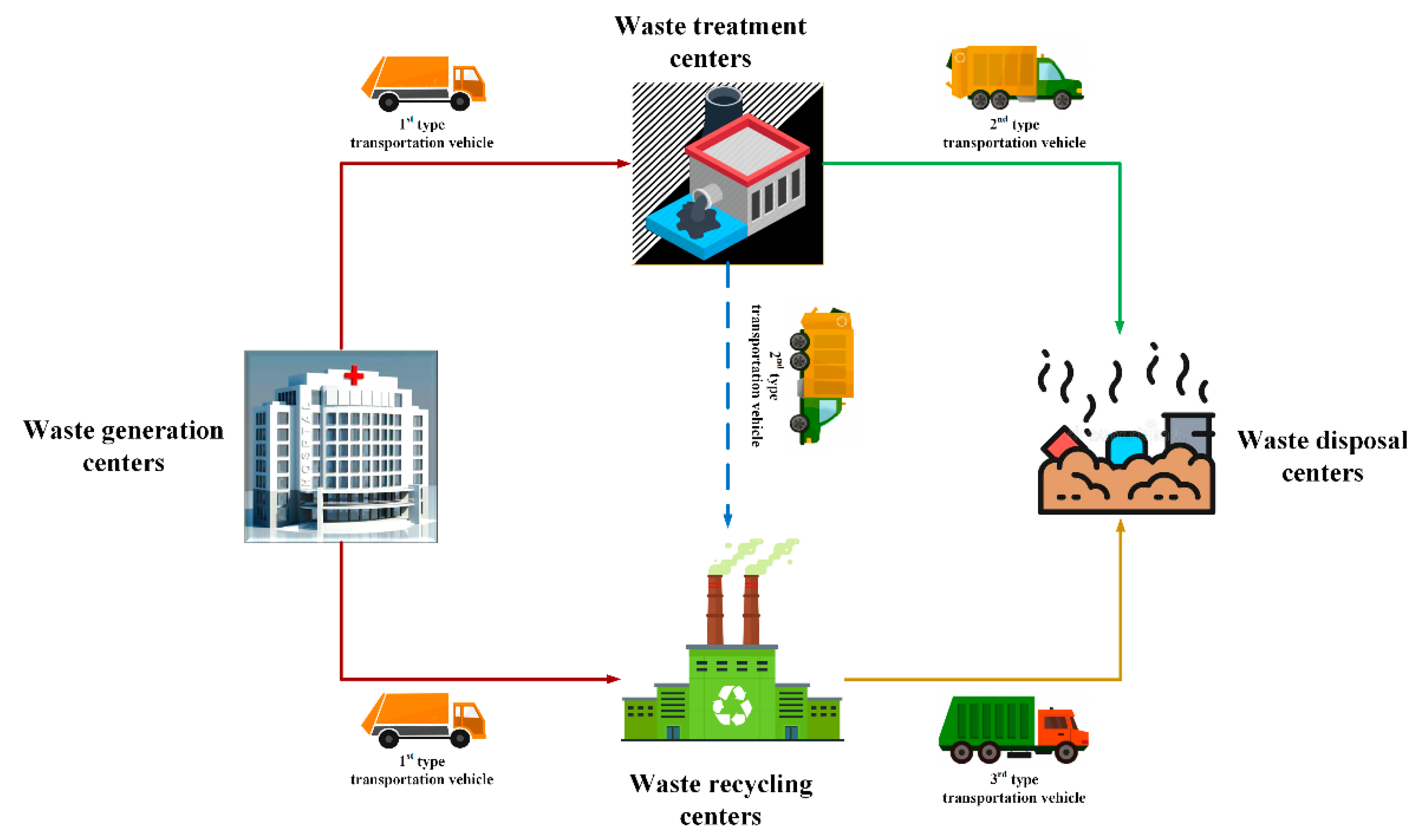
Figure 2.
Obtained results from the sensitivity analyses (Source: Author).

Figure 3.
Dispersion of objective functions against varying combinations of weights (Source: Author).
Figure 3.
Dispersion of objective functions against varying combinations of weights (Source: Author).

Table 1.
Summary of recent studies on sustainable waste network problems (Source: Author).
| Reference | Problem Characteristics | Problem Type | Objective Function | Methodology | ||||||
|---|---|---|---|---|---|---|---|---|---|---|
| Location | Allocation | Inventory | Transportation | Deterministic | Uncertain | Economic | Environmental | Social | ||
| Huang and Lin [20] | ✓ | ✓ | ✓ | Ant colony optimization algorithm for linear programming. | ||||||
| Mohsenizadeh et al. [29] | ✓ | ✓ | ✓ | ✓ | ✓ | ✓ | Bi-objective MILP | |||
| Ghiani et al. [33] | ✓ | ✓ | ✓ | ✓ | Mathematical modeling and heuristic algorithms. | |||||
| Ingheles et al. [34] | ✓ | ✓ | ✓ | ✓ | ✓ | Integrated linear programming and simulation modeling. | ||||
| López-Sánchez et al. [35] | ✓ | ✓ | ✓ | ✓ | Variable neighborhood search algorithm for a multi-objective optimization model. | |||||
| Yadav et al., [36] | ✓ | ✓ | ✓ | Interval-valued facility location model. | ||||||
| Habib et al. [37] | ✓ | ✓ | ✓ | ✓ | ✓ | ✓ | The multi-objective mathematical model under fuzzy environment. | |||
| Tirkolaee et al. [38] | ✓ | ✓ | ✓ | ✓ | ✓ | ✓ | ✓ | Robust optimization model. | ||
| Yu et al. [39] | ✓ | ✓ | ✓ | ✓ | ✓ | ✓ | Multi-objective mathematical model under stochastic environment. | |||
| Tirkolaee and Aydin [7] | ✓ | ✓ | ✓ | ✓ | ✓ | ✓ | Bi-objective mixed-integer linear programming. | |||
| Rathore and Sarmah [40] | ✓ | ✓ | ✓ | ✓ | ✓ | ✓ | ✓ | Multi-objective MILP and particle swarm optimization algorithm | ||
| Abdullah et al. [41] | ✓ | ✓ | ✓ | ✓ | ✓ | AHP and Multi-objective optimization model | ||||
| Asefi et al. [42] | ✓ | ✓ | ✓ | ✓ | ✓ | MILP model with variable neighborhood search | ||||
| Valizadeh et al. [43] | ✓ | ✓ | ✓ | ✓ | ✓ | ✓ | ✓ | Stochastic programming and Benders decomposition | ||
| Our study | ✓ | ✓ | ✓ | ✓ | ✓ | ✓ | ✓ | Multi-objective MILP model, Improved Multi-Choice Goal Programing, and Goal Attainment Method | ||
Table 2.
Information about the scale of the illustrative example (Source: Author).
| Scale | |G| | |T| | |R| | |D| | |H| | |W| | |K| | ||||
|---|---|---|---|---|---|---|---|---|---|---|---|
| Value | 20 | 6 | 6 | 6 | 7 | 3 | 7 | 7 | 7 | 7 | 7 |
Table 3.
Input parameters (Source: Author).
| Parameter | Value | Parameter | Value |
|---|---|---|---|
| uniform (1000,5000) | uniform (0.4,0.6) | ||
| uniform (0.4,0.6) | uniform (0.1,0.3) | ||
| uniform (180,000,220,000) | uniform (180,000,220,000) | ||
| uniform (180,000,220,000) | 15,000 | ||
| 10,000 | 8000 | ||
| uniform (10,100) | uniform (10,100) | ||
| uniform (10,100) | uniform (10,100) | ||
| uniform (10,100) | uniform (1,3) | ||
| uniform (1,3) | uniform (1,3) | ||
| uniform (1,3) | uniform (1,3) | ||
| uniform (2,5) | uniform (2,5) | ||
| uniform (2,5) | uniform (100,000,300,000) | ||
| uniform (100,000,300,000) | uniform (100,000,300,000) | ||
| uniform (1000,3000) | uniform (1000,3000) | ||
| uniform (1000,3000) | uniform (0.1,0.3) | ||
| uniform (0.1,0.3) | uniform (0.1,0.3) | ||
| uniform (0.1,0.3) | uniform (0.1,0.3) | ||
| uniformint (100,200) | uniformint (100,200) | ||
| uniformint (100,200) | 108 | ||
| (0.5, 0.3, 0.2) | (0.5, 0.3, 0.2) | ||
| (4.685512 × 10⁸, 523,663.149, 354) | (6.941714 × 10⁷, 282,966.137, 1715) | ||
| (6.941714 × 10⁷, 282,966.137, 1715) | (4.685512 × 10⁸, 523,663.149, 354) |
Table 4.
Computational results (Source: Author).
| Variable | Runtime (s) | ||||
|---|---|---|---|---|---|
| Value | 0.755 | 3.360903 × 10⁸ | 464,277.679 | 1684 | 5.27 |
Table 5.
Computational results (Source: Author).
| Variable | Solution Method | |
|---|---|---|
| IMCGP | GAM | |
| 3.360903 × 10⁸ | 8.130581 × 10⁷ | |
| 464,277.679 | 465,944.123 | |
| 1684 | 1666 | |
| Runtime (s) | 5.27 | 129.94 |
Table 6.
Results of the sensitivity analyses (Source: Author).
| Variables | |||||
|---|---|---|---|---|---|
| −20% | −10% | 0% | +10% | +20% | |
| 0.565 | 0.661 | 0.755 | 0.739 | - | |
| 2.806736 × 10⁸ | 3.129266 × 10⁸ | 3.360903 × 10⁸ | 3.147639 × 10⁸ | - | |
| 3.72241 × 10⁵ | 4.16891 × 10⁵ | 4.64277 × 10⁵ | 4.77076 × 10⁵ | - | |
| 1642 | 1642 | 1684 | 1646 | - | |
| Variables | |||||
| −20% | −10% | 0% | +10% | +20% | |
| - | 0.673 | 0.755 | 0.736 | - | |
| - | 3.080476 × 10⁸ | 3.360903 × 10⁸ | 3.351169 × 10⁸ | - | |
| - | 4.31786 × 10⁵ | 4.64277 × 10⁵ | 4.67695 × 10⁵ | - | |
| - | 1639 | 1684 | 1532 | - | |
| Variables | |||||
| −20% | −10% | 0% | +10% | +20% | |
| 0.693 | 0.650 | 0.755 | 0.713 | 0.747 | |
| 3.179353 × 10⁸ | 3.024876 × 10⁸ | 3.360903 × 10⁸ | 3.180348 × 10⁸ | 3.285489 × 10⁸ | |
| 4.44649 × 10⁵ | 4.32470 × 10⁵ | 4.64277 × 10⁵ | 4.59516 × 10⁵ | 4.71544 × 10⁵ | |
| 1583 | 1519 | 1684 | 1592 | 1629 | |
| Variables | |||||
| −20% | −10% | 0% | +10% | +20% | |
| 0.744 | 0.715 | 0.755 | 0.697 | 0.710 | |
| 3.511672 × 10⁸ | 3.239917 × 10⁸ | 3.360903 × 10⁸ | 3.320888 × 10⁸ | 3.354814 × 10⁸ | |
| 4.47964 × 10⁵ | 4.55373 × 10⁵ | 4.64277 × 10⁵ | 4.41305 × 10⁵ | 4.45765 × 10⁵ | |
| 1618 | 1589 | 1684 | 1514 | 1534 | |
Table 7.
Results obtained from different combinations of weights (Source: Author).
| (0.5, 0.3, 0.2) | 0.755 | 3.360903 × 10⁸ | 464,277.679 | 1684 |
| (0.5, 0.2, 0.3) | 0.734 | 3.400649 × 10⁸ | 437,537.653 | 1563 |
| (0.5, 0.4, 0.1) | 0.710 | 3.121720 × 10⁸ | 476,392.155 | 1497 |
| (0.6, 0.2, 0.2) | 0.809 | 3.825484 × 10⁸ | 456,083.940 | 1677 |
| (0.6, 0.3, 0.1) | 0.704 | 3.334987 × 10⁸ | 454,209.999 | 1631 |
| (0.6, 0.1, 0.3) | 0.699 | 3.364545 × 10⁸ | 400,897.908 | 1480 |
| (0.7, 0.2, 0.1) | 0.717 | 3.584374 × 10⁸ | 431,522.267 | 1532 |
| (0.7, 0.1, 0.2) | 0.738 | 3.595847 × 10⁸ | 417,509.831 | 1532 |
Publisher’s Note: MDPI stays neutral with regard to jurisdictional claims in published maps and institutional affiliations. |
© 2021 by the authors. Licensee MDPI, Basel, Switzerland. This article is an open access article distributed under the terms and conditions of the Creative Commons Attribution (CC BY) license (https://creativecommons.org/licenses/by/4.0/).
Share and Cite
MDPI and ACS Style
Torkayesh, A.E.; Vandchali, H.R.; Tirkolaee, E.B. Multi-Objective Optimization for Healthcare Waste Management Network Design with Sustainability Perspective. Sustainability 2021, 13, 8279. https://doi.org/10.3390/su13158279
AMA Style
Torkayesh AE, Vandchali HR, Tirkolaee EB. Multi-Objective Optimization for Healthcare Waste Management Network Design with Sustainability Perspective. Sustainability. 2021; 13(15):8279. https://doi.org/10.3390/su13158279
Chicago/Turabian StyleTorkayesh, Ali Ebadi, Hadi Rezaei Vandchali, and Erfan Babaee Tirkolaee. 2021. "Multi-Objective Optimization for Healthcare Waste Management Network Design with Sustainability Perspective" Sustainability 13, no. 15: 8279. https://doi.org/10.3390/su13158279
Note that from the first issue of 2016, this journal uses article numbers instead of page numbers. See further details here.