
Economic Development Policies and Land Use Changes in Thailand: From the Eastern Seaboard to the Eastern Economic Corridor


1
Faculty of Architecture and Planning, Rangsit Campus, Thammasat University, Pathum Thani 12121, Thailand
2
Department of Urban and Regional Planning, Faculty of Architecture, Chulalongkorn University, Bangkok 10330, Thailand
3
Regional, Urban, and Built Environment Analytics, Faculty of Architecture, Chulalongkorn University, Bangkok 10330, Thailand
*
Author to whom correspondence should be addressed.
Sustainability 2021, 13(11), 6153; https://doi.org/10.3390/su13116153
Submission received: 28 April 2021
/
Revised: 27 May 2021
/
Accepted: 28 May 2021
/
Published: 30 May 2021
(This article belongs to the Special Issue Urban Planning and Economic Development)
Abstract
:The Thai government’s project called “Eastern Economic Corridor (EEC)” was announced in 2016 to stimulate economic development and help the country escape from the middle-income trap. The project provides investment incentives for the private sector and the infrastructure development of land, rail, water, and air transportation. The EEC project encompasses three provinces in the eastern region of Thailand because of their strategic locations near deep seaports and natural resources in the Gulf of Thailand. Clearly, this policy will lead to dramatic changes in land uses and the livelihoods of the people in these three provinces. However, the extent to which land use changes will occur because of this project remains unclear. This study aims to analyze land use changes in the eastern region of Thailand using a Cellular Automata–Markov model. The results show that land uses of the coastal areas have become more urbanized than inland areas, which are primarily agricultural lands. The predicted land uses suggest shrinking agricultural lands of paddy fields, field crops, and horticulture lands but expanding perennial lands. These changes in land uses highlight challenges in urban administration and management as well as threats to Thailand’s agricultural cultures in the future.
1. Introduction
1.1. From the Eastern Seaboard
During the past several decades, the Thai economy has become rapidly industrialized. Once relying on agricultural products such as rice, wood, and sugar as well as simple processing industries in the 1960s–1970s, the economy has shifted toward export-driven industrialization since the mid-1980s. Rapid industrialization resulted from fiscal reforms and the aggressive promotion of industrial exports. Foreign Direct Investment (FDI) played a vital role in the strong economic growth of Thailand in the 1980s and 1990s [1].
In 1982, the Thai government launched the Eastern Seaboard Development Program (ESB) under the 5th National Economic and Social Development Plan (1982–1986). The project areas were in the eastern region of Thailand, covering three provinces, including Chonburi, Rayong, and Chachoengsao, chosen for their strategic locations near natural resources, such as natural gas, in the Gulf of Thailand. The goal of the ESB was to advance manufacturing industries from light to export-oriented heavy and commercialized manufacturing, for example, automobiles, electronics, and petrol chemical industries. The project consisted of several industrial estates, a deep seaport in Map Ta Phut, and a commercial port in Laem Chabang. Figure 1 illustrates the spatial distribution of the industrial estates, the deep seaport, and the commercial port in the region.
The ESB project has attracted a wide spectrum of businesses, ranging from agricultural processing to high-tech automobile assembling factories. As a result, the eastern region of Thailand has been an important economic driver of the country. In 2018, its Gross Regional Product (GRP) accounted for 17 percent of Thailand’s GDP [2]. As shown in Figure 2, the Gross Regional Product, in real terms, of the eastern region ranked the highest among the other regions (except for Bangkok) in Thailand. It also grew at a much higher rate than the other regions. In the early 90s, GRPs were similar across the regions. Two decades later, however, the real GRP of the eastern region increased from around 500,000 THB in 1994 to 1.7 million THB in 2018, around 10% annual growth, while the lowest GRP (the western region) grew slowly from about 100,000 THB in 1994 to 0.4 million THB. In 1994, the GRP of the eastern region was slightly higher than the second-highest GRP (the southern region), but in 2018, it was almost twice as much as the second-highest (the northeastern region).
Non-agricultural sectors contributed largely to the drastic growth of the GRP of the eastern region. Like the GRP, the eastern region’s GRP in non-agricultural sectors ranked second, following Bangkok. As shown in Figure 3 and Figure 4, the east’s non-agricultural sectors grew significantly from 1994 to 2018, and its growth pattern was very similar to the growth of the GRP. The non-agricultural sectors include manufacturing, construction, and services. On the other hand, the GRP in the eastern region’s agricultural sectors grew only slightly from 1994’s GRP. The eastern region ranked fourth in GRP in the agricultural sectors. The Southern region dominated the agricultural sectors, because it has rubber plantations, which have a relatively higher value than other agricultural products, as seen in Figure 5.
The ESB program has raised the per capita income level and reduced poverty in the region. As shown in Figure 5, the income per capita of the eastern region ranked first in 2018; it exceeded that of Bangkok from 2006 onward. The gaps of regional income per capita also widened, leaving the northeast and the north behind. Economic development policies such as the ESB have also driven land use changes in the region, for example, changes in land uses around Map Ta Phut Seaport in Rayong Province in the early 1980s. The development of the seaport has altered land uses around the port, transforming them from agricultural lands to urban areas. These transformations of land uses have had policy implications regarding urban and environmental management. Although much of the policy discussions have focused on its effectiveness regarding poverty reduction and increase in income per capita, its effects on land use changes—in terms of rapid urbanization and declining agricultural lands—have been largely underexamined.
1.2. To the Eastern Economic Corridor
The project called the “Eastern Economic Corridor (EEC)” was announced in 2016 under the 12th National Economic and Social Development Plan (2017–2021) in order to stimulate the economic development of the country. In particular, the project focuses on high-value-added industries such as automotive industries, electronics, robotics, aviation and logistics, biofuels and biochemicals, digital technologies, and medical hubs. Like the ESB, the EEC project covers three provinces in the eastern region: Chonburi, Rayong, and Chachoengsao (henceforth, EEC provinces).
The project has provided investment incentives for private sectors and public investments in land, rail, water, and air transportation infrastructures (Figure 6). A high-speed train route is planned, connecting two major airports in Bangkok (Don Muang Airport and Suvarnabhumi Airport) to the new airport (U-Tapao Airport) in the region. Industrial clusters and new cities are planned and promoted.
Unlike other area-based industrial estates where local municipalities are responsible for managing the area, as a public agency, the Eastern Economic Corridor Office of Thailand (EECO) was established to facilitate investments and coordinate with local authorities under the EEC Act BE 2561 (2018). In addition, the Act specifies three levels of planning frameworks: (1) the EEC Regional Plan and Provincial Plan, (2) the Town Comprehensive Plan, and (3) the Specific Plan (Figure 7). The Regional and Provincial Plan sets the direction of the development at the regional and provincial levels, such as the development of infrastructure networks. The Town Comprehensive Plan defines zoning control for urban areas, whereas the Specific Plan specifies the development plans, including area master plans, land readjustment plans, and implementation processes. The Department of Public Works and Town and Country Planning (DPT), under the Ministry of the Interior, is responsible for preparing these plans of the EEC.
1.3. Economic Development Policies and Land Use Changes
The role of the government in economic development has long been a topic of debate in economic literature. Two extreme views of the role of the government depict one economy with extreme total government control and the other with a laissez-faire style of control. A third view, however, has emerged as the middle ground between these two extremes, where the economic development roles of the government and the private sector are balanced [3]. Fundamentally, the role of the government is to establish infrastructures, such as the physical, environmental, social, and financial infrastructures of the economy, in order to facilitate the functioning of the market so that the government’s central role of increasing wealth and improving living standards can be fulfilled [3,4]. As Stiglitz put it, “well-designed government actions can improve living standards whenever there are imperfections of information or competition or incomplete markets” [3].
For many developing countries, economic development policies have been driven by industrialization, whereby the governments have provided firms with strong financial and non-financial incentives [3]. Industrial policies have been viewed as a silver bullet for stimulating economic growth, since many empirical studies have shown that industrialization is positively correlated with economic growth [1,5,6].
Industrialization, however, has been strongly linked to urbanization. Evidence in China, for example, has shown that industrialization has significantly contributed to urban expansions [7]. Countries relying heavily on natural resource exports are also highly linked to urban expansions. Specifically, countries in Asia with a high percentage share of manufacturing and services in GDP are positively correlated with the degree of urbanization [8]. Industrialization policies clearly have strong implications for changes in land uses [9].
As an export-oriented market, the EEC project in Thailand has been expected to bring dramatic changes in the economic landscape. In particular, land uses in the region will drastically change from new infrastructure investments to the emergence of new settlements or cities. Nevertheless, the effects of the EEC on land use changes have not yet been well understood.
The objectives of this study are two-pronged: (1) to examine historical land cover changes of EEC provinces in Thailand and (2) to predict future land uses of these provinces by examining historical land use changes. This study analyzes land use changes in the EEC provinces, using a Cellular Automata–Markov (CA–Markov) model. The CA–Markov model is widely used in analyzing land use–land cover change patterns in the past to predict future land use changes. Previous empirical studies on land use changes in Thailand focused on major cities like the Bangkok Metropolitan Region [10] and Hua Hin [11], but not many studies have focused on the EEC. To the best of our knowledge, this analysis is the first of only a few attempts so far to examine the effects of the EEC policy on land use changes in the EEC provinces.
2. Materials and Methods
2.1. Spatial Data
The geospatial data of land use in the EEC provinces is obtained from the Soil Service Repository of Land Development Department, Ministry of Agriculture and Cooperatives of Thailand [12]. The land use data are based on the GISagro database of the Geo-Informatics and Space Technology Development Agency (GISTDA) of Thailand. The GISagro dataset is assembled on multiple sources of remote sensing data, including LANDSAT-7, THEOS, RADARSAT, QuickBird, SPOT-5and IKONOS [13]. The data are in a shapefile format that can be visualized and processed in ArcGIS. These multi-year data include 2007, 2010, 2012, and 2016 (Figure 8). The analysis is limited to these years because of the constraint in data availability.
The land use data provide detailed classification of land use types on three levels. The first level consists of five major types of land use: (1) urban and built-up land, (2) agricultural land, (3) forest land, (4) water bodies, and (5) miscellaneous land. The second level provides greater classifications of land use of the first level. The third level gives the finest details of land use classification. For example, perennial classification in the second level may be further classified as mixed perennial, Para rubber, oil palm, bamboo, eucalyptus, or teak (this is not an exhaustive list). However, the level 3 land use classification is not available in every year of the data set. Therefore, the analysis is limited to the second level of land use classification.
Table 1 shows the description of land use classification in the analysis. Level II classifications are grouped into 9 types of land use. Out of these groups, five are agricultural lands because different crops tend to have different changing patterns. For example, rice paddy fields are cultivated in the rice harvesting season, which is between August and December in Thailand. Field crops, on the other hand, are cultivated year-round. While crop changes are observed for paddy fields and field crops, there are not many changes in perennials.
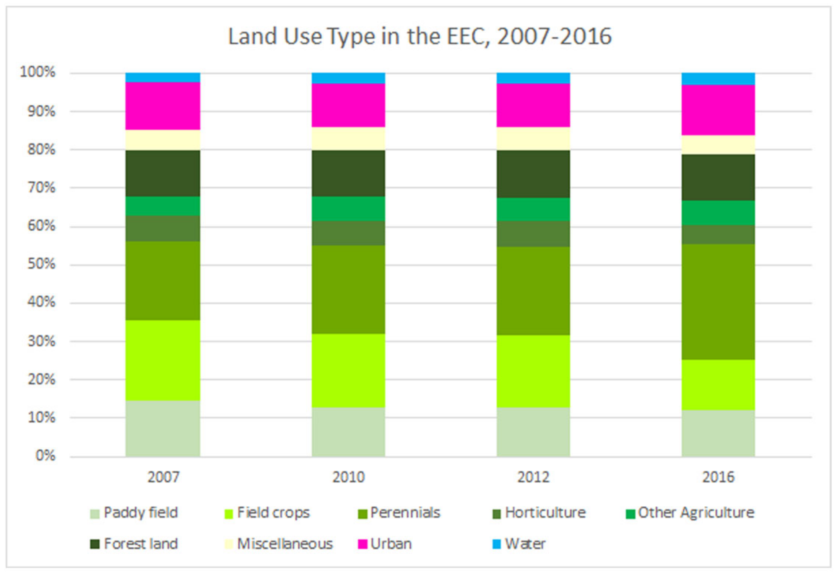
Although the economy is manufacturing-based, land uses in the EEC are primarily agricultural lands. Altogether, agricultural lands accounted for 67 percent in the EEC in 2016. Urban and built-up lands accounted for 13 percent, and forest lands accounted for 12 percent. Miscellaneous lands and water bodies accounted for 5 and 3 percent, respectively (Figure 9).
The EEC Provinces were not equally urbanized. Chon Buri had the largest urbanized lands with an area of over 900 square kilometers (347 square miles) in 2016, accounting for 20 percent of total land areas. Rayong was the second largest urbanized province in the East, with urban areas of 484 square kilometers in 2016 (13 percent of total areas). Chachoengsao had the smallest share of urban areas at 412 square kilometers or 8 percent of the total areas. One caveat of the study should be mentioned, however. Since GISagro data are drawn from several remote sensing data sources, it is possible that the land use data of 2007 and 2016 may come from a different source than that of the 2010 and 2012 data.
2.2. Land Use Change Model
There are many approaches to analyzing land use changes and predicting future land use. Land use models can be classified into four categories: (1) statistical and econometric models, (2) spatial interaction models, (3) optimization models, and (4) integrated models [15]. With the improvement in Geographic Information Systems and remote sensing, spatially and temporally explicit models of land use changes such as Cellular Automata–Markov (CA–Markov) have been widely used in land use change and land use simulation (for example, [10,16,17,18]. A CA–Markov model combines spatial neighboring effects in a Cellular Automata model with temporal transition in a Markov model.
Based on the concept of von Neumann’s spatial structure, Cellular Automata (CA) is a land use/land cover model that has been widely used since the 1960s because of its simplicity and independence of theoretical hypotheses [19]. A two-dimensional lattice of cells represents spatial dimensions in a CA model. These cells’ characteristics can be changed in each state according to some transition rules defined in the model [20]. As such, a CA model can incorporate changes in both space and time.
A typical CA model process is defined in iteration; for each iteration, a status or the characteristics of a cell may change or remain unchanged, depending on the status of its adjacent neighbor cells. These neighbors can be characterized in two different ways: (1) the Moore neighborhood and (2) the von Neumann neighborhood. The Moore neighborhood takes all eight cells surrounding the cell into consideration, while the von Neumann neighborhood consists of four cells in the North, East, South, and West [19].
The other component of a CA–Markov model is a Markov model. A Markov Land Use/Land Cover (LULC) model takes into consideration temporal transitions through a Markovian process. In a Markovian process, the status of a cell in period t + 1 is characterized by its status in the previous period, t. The change from one period to another is defined by a transition probability matrix [21]. Suppose P denotes a probability of land use change among k land use classifications, which can be described in a matrix as follows:
where Pij denotes the probability of changing from a status i to a status j. The probability has the following properties:
P = Pij,
∑j=1Pij = 1,
0 ≤ Pij ≤ 1.
Therefore, a Markov model has the following property:
where P(n) denotes a probability in period n, and P(0) denotes a probability from the land use data. With these properties of the probability transition matrix, a Markov model can be used to predict future land uses from the current ones [21].
P(n) = P(n−1)Pij = P(0) Pijn,
The CA–Markov model is widely used to analyze land use/land cover change because of its practicality advantages and spatio-temporal explicitness. At least two time periods of land use data are required to successfully run the model, which is very convenient for areas where land use data are not frequently available. However, the CA–Markov has some disadvantages. Because the future land use is predicted from previous land use patterns, the model is more suitable for predicting land use changes in the short and medium terms than in the long term. Nevertheless, for the purpose of this analysis, the CA–Markov is suitable because the short and medium-term land use changes are the focus of the land use prediction.
In this analysis, a CA–Markov model was run using TerrSet Geospatial Monitoring and Modeling Software. This software supports GIS image processing as well as geospatial tools that can analyze land use changes [22]. Figure 10 illustrates the procedure of the analysis. Three years of land use data (2007, 2012, and 2016) are model inputs to analyze short-term changes (five-year period from 2007 to 2012) and medium-term changes (nine-year period from 2007 to 2016). The predicted 2016 land use from short-term changes was compared with actual 2016 land use to validate the model, using statistical independence tests [23], because the land use to be used for comparison purposes should not be used for calibration [24]. Using the validated model, land use prediction was simulated for a short term (2022) and medium term (2027) with a specification of urban growth from the EEC project.
3. Results
3.1. Land Use Change
A CA–Markov model of land use gives two major outputs: (1) a Markov transition probability matrix of different land use types and (2) Markovian conditional probability maps. The Markov transition probability matrix of land use change in the short term is shown in Table 2 and in the medium term in Table 3. The values in each row of the matrix can be summed up to one, meaning that they are probabilities of turning from one type of land use in the first time period (denoted in rows) into other types of land use in the second time period (denoted in columns). The diagonal cells represent the probability of land use remaining the same. Comparison of the Markov transition matrix in the short run and in the medium run shows changing patterns of land use in different time spans. For example, the probability of a rice paddy field turning into an urban land is 2.2 percent in the short term but increases to 5.7 percent in the medium term. Likewise, miscellaneous lands have a higher probability of being converted to urban areas in the medium term than in the short term. Urban expansion is impacted primarily due to the conversion of miscellaneous lands and agriculture lands such as paddy fields, crops, and horticulture, suggesting that urban lands come from both brownfield and greenfield developments.
In addition to the likelihood of land use changes in the Markov transition probability matrix, Markov conditional probability maps show spatial locations with probabilities being in each land use class. Markov conditional probability maps of 2007–2012 and 2007–2016 transitions are shown in Figure 11 and Figure 12, respectively. As can be seen, the Markov conditional probability of being paddy fields is high in areas in Chachoengsao Province in the northwest of the region, whereas the conditional probability of being crop fields and perennial lands is high in the central and west areas of the region. Urban areas are primarily along coastal areas.
3.2. Model Validation
The CA–Markov model is validated by comparing the predicted 2016 land use to the actual 2016 land use at the pixel level, using the cross-tabulation analysis. A Chi-square test and Cramer’s V are used in the pixel cross-tabulation to test the interdependence between actual and predicted land uses, while the Overall Kappa is used for proportional cross-tabulation to validate model prediction of land use changes [24,25,26]. The value of Cramer’s V is acceptable when its value is greater than 0.5. Preferable Overall Kappa should be above 0.8 [26,27]. The test statistics are reported in Table 4. Overall, the tests show satisfactory results, with Cremer’s V of 0.8183 and Overall Kappa of 0.8457.
3.3. Predicted Land Use
With the Markov transitional probability matrix and Markov conditional probability maps, we can predict future land uses. In this case, land uses in 2022 and 2027 were simulated based on land use changes from 2007–2012 and validated with actual 2016 land use. The results of the simulation are shown in Figure 13. As can be seen, the coastal areas are still primarily urban and built-up lands, with some urban developments in inland areas in the western part of the region.
As shown in Table 5, the model predicts the growth in perennials, other agriculture, urban, and water land uses, with an average annual growth of 5.15%, 3.38%, 2.40%, and 2.67%, respectively. On the other hand, by 2027, other agricultural lands, including paddy fields, field crops, and horticulture, are expected to have declined, with an annual average of −2.86%, −4.05%, and −4.37%, respectively. Forest lands and miscellaneous lands are also expected to be declining slightly with an annual average of −0.09% and −0.57%.
4. Discussion
The results show that urban areas in the EEC are expected to expand unevenly across the region, primarily along the coastal areas. These urban expansions from economic development policies have many implications in terms of physical infrastructures such as roads, sewage systems, and electricity, and in terms of social infrastructures such as schools, health care services, and hospitals. These services should be sufficiently provided for growing urban populations.
Another policy implication of urban expansions relates to the administration and management of urban areas. As shown in Figure 14, urban spatial growths extend beyond just one administrative boundary. This could be problematic for appropriate fiscal and resource allocations among these municipalities, both in terms of natural resources and man-made ones. Thus, regional and urban plans should be integrative among several municipalities when urban areas expand beyond more than two local administrative boundaries.
In addition, the land use change simulation predicts a decline in agricultural lands, particularly paddy fields, field crops, and horticulture. These trends present a threat not only to the food security for human beings, but also to Thailand’s agricultural cultures. Rice cultivation has long been a part of Thai agriculture cultures, and rice is one of Thailand’s main agricultural products. A decrease in paddy fields could lead to declining rice production as well as a disappearing rice cultivation culture.
Further, the eastern region of Thailand is well-known for its geographical identities (similar to “terroir” in wine production) of orchards and tropical fruits such as durian, mangosteen, and rambutan. Durian, in particular, is a major exported fruit of Thailand. In the first half of 2019, the value of durian exports was US$817 million, accounting for 44% of the total Thai fruit exports [28]. A decrease in horticultural lands and orchards could lead to a lower level of such high-value agricultural productions. Since Thailand is one of the world’s leading food exporters, agricultural land uses should be carefully planned for in the future. Land use planning at the regional level (EEC Plan) and the Town Comprehensive Plan are essential to ensure the balance between urban growth and changes in agricultural lands.
A draft of the EEC land use plan for 2037 was announced in 2019 (Figure 15). As can be seen, high-density urban areas are primarily along the coastal areas, which are supported by the results of this study. Industrial lands (shown in purple) are planned in the inner lands and buffered to urban areas by land reform zones announced in Royal Decree. Land use regulations for these land reform zones are primarily for agricultural purposes. Therefore, the zones could serve as a natural boundary to urban areas as well as a buffer between industrial and residential lands. In particular, the concept of controlling greenfield developments and promoting brownfield developments should be introduced in the regional and provincial plans for spatial developments in the urban–rural fringe.
It is also worth noting that the prediction of an increase in perennials is based on its increasing trend in the past, which was a result of the high commodities and market prices of such perennial agricultural products. Examples of such perennials in the region include Para rubber, palm oil, and eucalyptus. Para rubber, particularly, has been widely grown not only in the EEC region, but also in the rest of Thailand during the past few decades because of its high prices, together with the Thai government’s policy to promote rubber cultivation. Because of the increase in rubber prices in the 2000s, Para rubber has become one of the major crops in the eastern region, along with tropical fruit orchards. The Para rubber price reached its peak in 2011 and has been steadily declining since then [30]. However, Para rubber gained the largest share in agricultural lands in 2016 while the rubber price was at its lowest, suggesting that land use changes are likely to be lagging behind changes in prices. Thus, our timeframe of land use change may not be able to capture the decline of perennials due to its decline in prices, such that the interdependence of commodity prices and land use changes could result in a knowledge gap that can be explored in the future.
5. Conclusions
Land use changes have often been driven by economic development policies. In the past few decades, the Eastern Seaboard Development Program (ESB) has shaped land use changes in three provinces in the east of Thailand, namely Chonburi, Rayong, and Chachoengsao. These provinces have been transformed from agricultural lands to industrial and urban land uses. In 2016, the Eastern Economic Corridor (EEC) Project was announced as a strategy to promote higher investments in high-tech industries and innovations. Little is known, however, about the effects of the EEC on the future land uses in the region.
This analysis employs the CA–Markov land use model to examine land use changes and to predict short- and medium-term future land use in the EEC region. The model also compares land use transition probabilities of two time periods in the past. The analysis reveals that agricultural land uses are less likely to maintain their uses in the medium term than in the short term. Forest lands remain unchanged in both short and medium terms, and urban lands tend to be converted from miscellaneous lands.
The predicted future land uses show that urban expansions are primarily along coastal areas of the region. The growth of urban lands implies higher provisions of both physical and social infrastructures to serve the growing urban population. It also suggests integrative planning among several municipalities at the regional and urban levels. On the other hand, the model predicts the expansion of commodity crops like perennials, but a decline in other agricultural lands. These shrinking agricultural lands present threats to agriculture cultivation cultures, especially rice cultivation and horticulture, which have long been an important part of Thai agricultural cultures. Thus, future urbanization driven by infrastructure investments and industrialization policies like the ESB and the EEC should be carefully planned for, with consideration to urban administration and management as well as the preservation of agricultural lands. Some limitations of this analysis should be noted. First, future land uses have been path-dependent on the historical trend since 2007. Thus, the model may not be able to fully capture patterns of land use changes since the launch of the ESB, which began in the 1980s. Nonetheless, these current land use change patterns may serve as a basis for assessing the impacts of the EEC on future land uses in the region. Second, the land use change model does not incorporate other socio-economic factors such as land ownership and prices of agricultural products, which could be key factors driving land use changes. Several agricultural commodities such as rice, Para rubber, palm oil, and tropical fruits have been major agricultural exports of Thailand and major crops in the region. The interdependence of commodity prices and land use changes could be a topic for future investigation. Finally, another missing factor affecting land use changes is the individual decisions of landowners, for example, whether to maintain current uses, convert their lands to other uses, or sell their lands. These autonomous land use decisions may collectively alter land use patterns in the future. This issue may be well-addressed in an agent-based model [31], which could be another direction of future research.
Author Contributions
Conceptualization, N.T. and S.A.; methodology, N.T. and S.A.; software, N.T. and S.A.; validation, N.T. and S.A.; formal analysis, N.T. and S.A.; investigation, N.T. and S.A.; resources, N.T. and S.A.; writing—original draft preparation, N.T. and S.A.; writing—review and editing, N.T. and S.A.; visualization, N.T. and S.A.; funding acquisition, N.T. All authors have read and agreed to the published version of the manuscript.
Funding
This study was supported by Thammasat University Research Fund, Contract No. TUFT 10/2562 and the Grants for Development of New Faculty Staff, Ratchadaphiseksomphot Endowment Fund, Chulalongkorn University, Contract No. DNS 60-055-25-002-1.
Institutional Review Board Statement
Not applicable.
Informed Consent Statement
Not applicable.
Data Availability Statement
Publicly available datasets were analyzed in this study. This data can be found here: http://dinonline.ldd.go.th/ (accessed on 29 May 2021).
Acknowledgments
The authors would like to thank the research support team at Regional, Urban, and Built Environment Analytics, Faculty of Architecture, Chulalongkorn University, namely, Chachanok Rukbanglaem, Korrakot Positlimpakul, and Oraya Pienrakkarn.
Conflicts of Interest
The authors declare no conflict of interest.
References
- Hussey, A. Rapid Industrialization in Thailand 1986–1991. Geogr. Rev. 1993, 83, 14–28. [Google Scholar] [CrossRef]
- [NESDB] Gross Regional and Provincial Product Chain Volume Measures 2018 Edition. Office of the National Economic and Social Development Board. Available online: https://www.nesdc.go.th/main.php?filename=gross_regional (accessed on 23 February 2021).
- Stiglitz, J.E. The role of government in economic development. In Annual World Bank Conference on Development Economics 1996; Bruno, M., Pleskovic, B., Eds.; The World Bank: Washington, DC, USA, 1996; pp. 11–23. ISBN 0821337866. [Google Scholar]
- Stiglitz, J.E. Government, Financial Markets and Economic Development. Natl. Bur. Econ. Res. 1991, 3669, 1–40. Available online: http://www.nber.org/papers/w3669.pdf (accessed on 23 February 2021).
- Kim, J.I.; Lau, L.J. The sources of economic growth of the east asian newly industrialized countries. J. Jpn. Int. Econ. 1994, 8, 235–271. [Google Scholar] [CrossRef]
- Salvatore, D. International trade policies, industrialization, and economic development. Int. Trade J. 1996, 10, 21–47. [Google Scholar] [CrossRef]
- Deng, X.; Huang, J.; Rozelle, S.; Uchida, E. Growth, population and industrialization, and urban land expansion of China. J. Urban Econ. 2008, 63, 96–115. [Google Scholar] [CrossRef]
- Gollin, D.; Jedwab, R.; Vollrath, D. Urbanization with and without industrialization. J. Econ. Growth 2016, 21, 35–70. [Google Scholar] [CrossRef]
- Kim, J.H. Linking land use planning and regulation to economic development: A literature review. J. Plan. Lit. 2011, 26, 35–47. [Google Scholar]
- Losiri, C.; Nagai, M.; Ninsawat, S.; Shrestha, R.P. Modeling urban expansion in Bangkok Metropolitan region using demographic-economic data through cellular Automata-Markov Chain and Multi-Layer Perceptron-Markov Chain models. Sustainability 2016, 8, 686. [Google Scholar] [CrossRef] [Green Version]
- Kityuttachai, K.; Tripathi, N.; Tipdecho, T.; Shrestha, R. CA-Markov Analysis of Constrained Coastal Urban Growth Modeling: Hua Hin Seaside City, Thailand. Sustainability 2013, 5, 1480–1500. [Google Scholar] [CrossRef] [Green Version]
- Land Development Department. Available online: http://webapp.ldd.go.th/Soilservice/ (accessed on 15 November 2017).
- [GISTDA] The Role of Geographic Information Systems in Agricultural Management. Technical Reports of Geo-Informatics and Space Technology Development Agency. Available online: http://slb-gis.envi.psu.ac.th/home/images/download/Data-dictionary/theme08.pdf (accessed on 22 August 2018).
- [GISTDA] Classification Standard of Fundamental Geographic Data Set (FGDS). Technical Reports of Geo-Informatics and Space Technology Development Agency. Available online: https://sites.google.com/site/fgdsservice/home/fgds (accessed on 22 August 2018).
- Briassoulis, H. Analysis of land use change: Theoretical and modeling approaches. In Web Book of Regional Science; West Virginia University: Morgantown, WV, USA, 2000. [Google Scholar]
- Sang, L.; Zhang, C.; Yang, J.; Zhu, D.; Yun, W. Simulation of land use spatial pattern of towns and villages based on CA-Markov model. Math. Comput. Model. 2011, 54, 938–943. [Google Scholar] [CrossRef]
- Yang, X.; Zheng, X.-Q.; Chen, R. A land use change model: Integrating landscape pattern indexes and Markov-CA. Ecol. Model 2014, 283, 1–7. [Google Scholar] [CrossRef]
- Yirsaw, E.; Wu, W.; Shi, X.; Temesgen, H.; Bekele, B. Land Use/Land Cover Change Modeling and the Prediction of Subsequent Changes in Ecosystem Service Values in a Coastal Area of China, the Su-Xi-Chang Region. Sustainability 2017, 9, 1204. [Google Scholar] [CrossRef] [Green Version]
- Batty, M. Cellular Automata and Urban Form: A Primer. J. Am. Plan. Assoc. 1997, 63, 266–274. [Google Scholar] [CrossRef]
- White, R.; Engelen, G. Cellular automata and fractal urban form: A cellular modeling approach to the evolution of urban land-use patterns. Environ. Plan. A 1993, 25, 1175–1199. [Google Scholar] [CrossRef] [Green Version]
- Hyandye, C.; Martz, L.W. Markovian and cellular automata land-use change predictive model of the Usangu Catchment. Int. J. Remote Sens. 2017, 38, 64–81. [Google Scholar] [CrossRef]
- TerrSet Geospatial Monitoring and Modeling Software. Available online: https://clarklabs.org/terrset/ (accessed on 15 November 2017).
- Gil, R.P.; Jeffrey, M. Comparison of the structure and accuracy of two land change models. Int. J. Geogr. Inf. Syst. 2005, 19, 243–265. [Google Scholar] [CrossRef]
- Pontius, R.G.; Schneider, L. Land-cover change model validation by an ROC method for the Ipswich watershed, Massachusetts, USA. Agric. Ecosyst. Environ. 2001, 85, 239–248. [Google Scholar] [CrossRef]
- Mondal, M.S.; Sharma, N.; Garg, P.K.; Kappas, M. Statistical independence test and validation of CA Markov land use land cover (LULC) prediction results. Egypt. J. Remote Sens. Sp. Sci. 2016, 19, 259–272. [Google Scholar] [CrossRef] [Green Version]
- Hamad, R.; Balzter, H.; Kolo, K. Predicting Land Use/Land Cover Changes Using a CA-Markov Model under Two Different Scenarios. Sustainability 2018, 10, 3421. [Google Scholar] [CrossRef] [Green Version]
- Eastman, J.R. IDRISI Andes Tutorial; Clark Labs: Worcester, MA, USA, 2006. [Google Scholar]
- Bangkok Post. Thailand Champion of Durian Exports. Available online: https://www.bangkokpost.com/business/1735595/thailand-champion-of-durian-exports (accessed on 15 September 2019).
- [EECO] Overall Land Use Plan. Eastern Economic Corridor Office of Thailand. Available online: https://eeco.or.th/th/overall-land-use-plan (accessed on 26 May 2021).
- Statistics of Para Rubber Plantation in Thailand 2011–2013. Office of Agricultural Economics. Available online: http://www.rubberthai.com/statistic/stat_index.htm (accessed on 15 November 2017).
- Macal, C.M.; North, M.J. Tutorial on agent-based modelling and simulation. J. Simul. 2010, 4, 151–162. [Google Scholar] [CrossRef]
Figure 1.
Chonburi, Rayong, and Chachoengsao Provinces.

Figure 2.
Gross regional product chain volume measures, 1994–2018 (Source: Office of the National Economic and Social Development Board (NESDB)).
Figure 2.
Gross regional product chain volume measures, 1994–2018 (Source: Office of the National Economic and Social Development Board (NESDB)).

Figure 3.
Gross regional product chain volume measures in non-agricultural sectors, 1994–2018 (Source: NESDB).
Figure 3.
Gross regional product chain volume measures in non-agricultural sectors, 1994–2018 (Source: NESDB).

Figure 4.
Gross regional product chain volume measures in agricultural sectors, 1994–2018 (Source: NESDB).
Figure 4.
Gross regional product chain volume measures in agricultural sectors, 1994–2018 (Source: NESDB).

Figure 5.
Income per capita at current market price by region, 1994–2018 (Source: NESDB).

Figure 6.
Infrastructure and urban development in EEC (Source: adapted from Thailand Board of Investment, 2019).
Figure 6.
Infrastructure and urban development in EEC (Source: adapted from Thailand Board of Investment, 2019).

Figure 7.
Planning tier of EEC Act.

Figure 8.
Land use in the EEC Provinces, 2007–2016.

Figure 9.
Distribution of land use type in the EEC, 2007–2016.

Figure 10.
Overall procedure of the analysis.

Figure 11.
Markovian conditional probability maps, 2007–2012.

Figure 12.
Markovian conditional probability maps, 2007–2016.

Figure 13.
Predicted land use of the EEC, 2022 and 2027.

Figure 14.
Urban areas and municipality boundaries.

Figure 15.
EEC land use plan for 2037. (Source: adapted from EECO [29]).
Figure 15.
EEC land use plan for 2037. (Source: adapted from EECO [29]).


Table 1.
Land use classification Description.
| Class | Land Use | Level II Classification |
|---|---|---|
| 1 | Paddy field | Paddy field |
| 2 | Field crops | Field crop |
| 3 | Perennials | Perennial |
| 4 | Horticulture | Horticulture |
| Orchard | ||
| 5 | Other agricultural land | Swidden cultivation |
| Pasture and farmhouse | ||
| Aquatic plant | ||
| Aquacultural land | ||
| Integrated farm | ||
| 6 | Forest land | Evergreen forest |
| Deciduous forest | ||
| Mangrove forest | ||
| Swamp forest | ||
| Forest plantation | ||
| Agro-forestry | ||
| Beach forest | ||
| 7 | Miscellaneous land | Rangeland and scrub |
| Marsh and swamp | ||
| Mine and pit | ||
| Other miscellaneous land | ||
| Salt flat | ||
| Beach | ||
| Garbage dump | ||
| 8 | Urban and built-up land | Urban and commercial area |
| Residential area | ||
| Governmental and institutional land | ||
| Transportation, communication, and utilities | ||
| Industrial land | ||
| Other built-up land | ||
| Golf course | ||
| 9 | Water body | Natural water body |
| Artificial water body |
Source: Adapted from FGDS Data description [14].
Table 2.
Markov transition probability matrix, 2007–2012.
| 2012 | ||||||||||
|---|---|---|---|---|---|---|---|---|---|---|
| Paddy | Crop | Peren. | Horti. | Other | Forest | Misc | Urban | Water | ||
| 2007 | Paddy | 0.825 | 0.012 | 0.015 | 0.004 | 0.085 | 0.001 | 0.030 | 0.022 | 0.006 |
| Field Crop | 0.005 | 0.787 | 0.144 | 0.013 | 0.002 | 0.002 | 0.023 | 0.022 | 0.003 | |
| Perennials | 0.001 | 0.072 | 0.893 | 0.011 | 0.002 | 0.006 | 0.008 | 0.006 | 0.001 | |
| Horticulture | 0.006 | 0.068 | 0.142 | 0.698 | 0.019 | 0.005 | 0.032 | 0.027 | 0.003 | |
| Other | 0.060 | 0.004 | 0.005 | 0.003 | 0.882 | 0.002 | 0.018 | 0.022 | 0.005 | |
| Forest | 0.000 | 0.002 | 0.010 | 0.002 | 0.001 | 0.977 | 0.003 | 0.004 | 0.000 | |
| Misc | 0.011 | 0.064 | 0.040 | 0.010 | 0.019 | 0.043 | 0.740 | 0.052 | 0.022 | |
| Urban | 0.012 | 0.021 | 0.013 | 0.094 | 0.023 | 0.004 | 0.035 | 0.790 | 0.008 | |
| Water | 0.002 | 0.009 | 0.005 | 0.002 | 0.009 | 0.002 | 0.035 | 0.013 | 0.925 | |
Table 3.
Markov transition probability matrix, 2007–2016.
| 2016 | ||||||||||
|---|---|---|---|---|---|---|---|---|---|---|
| Paddy | Crop | Peren. | Horti. | Other | Forest | Misc | Urban | Water | ||
| 2007 | Paddy | 0.694 | 0.030 | 0.049 | 0.011 | 0.096 | 0.002 | 0.049 | 0.057 | 0.012 |
| Field Crop | 0.010 | 0.468 | 0.365 | 0.032 | 0.005 | 0.003 | 0.030 | 0.080 | 0.008 | |
| Perennials | 0.002 | 0.076 | 0.857 | 0.016 | 0.003 | 0.010 | 0.009 | 0.019 | 0.009 | |
| Horticulture | 0.011 | 0.115 | 0.314 | 0.392 | 0.026 | 0.003 | 0.032 | 0.099 | 0.008 | |
| Other | 0.091 | 0.009 | 0.016 | 0.009 | 0.787 | 0.003 | 0.028 | 0.047 | 0.011 | |
| Forest | 0.000 | 0.008 | 0.033 | 0.002 | 0.002 | 0.937 | 0.007 | 0.010 | 0.001 | |
| Misc | 0.015 | 0.108 | 0.111 | 0.016 | 0.030 | 0.039 | 0.473 | 0.171 | 0.039 | |
| Urban | 0.015 | 0.027 | 0.037 | 0.064 | 0.024 | 0.008 | 0.039 | 0.775 | 0.011 | |
| Water | 0.004 | 0.013 | 0.012 | 0.002 | 0.012 | 0.003 | 0.039 | 0.045 | 0.870 | |
Table 4.
Test statistics for model validation.
| Test Statistics | Value |
|---|---|
| Pixel Cross-tabulation | |
| Chi-square | 144,058,288 |
| Degree of Freedom | 81 |
| P-level | 0.00 |
| Cremer’s V | 0.8183 |
| Proportional Cross-tabulation | |
| Overall Kappa | 0.8457 |
Table 5.
Distribution of predicted land use of the EEC (Square Kilometer), 2022 and 2027.
| Land Use Classification | 2007 | 2012 | 2016 | 2022p | 2027p | Annual % Change |
|---|---|---|---|---|---|---|
| Paddy field | 1953.15 | 1701.31 | 1571.62 | 1402.03 | 1395.24 | −2.86 |
| Field crops | 2749.92 | 2534.82 | 1826.12 | 1678.43 | 1636.31 | −4.05 |
| Perennials | 2734.09 | 3067.30 | 3966.04 | 4167.78 | 4142.66 | 5.15 |
| Horticulture | 903.79 | 873.68 | 664.32 | 514.80 | 508.89 | −4.37 |
| Other agriculture | 676.19 | 845.98 | 839.87 | 917.15 | 904.78 | 3.38 |
| Forest land | 1643.38 | 1670.26 | 1633.34 | 1652.19 | 1629.04 | −0.09 |
| Misc. | 700.10 | 776.64 | 622.52 | 661.28 | 660.21 | −0.57 |
| Urban | 1674.49 | 1529.32 | 1820.82 | 1945.17 | 2076.10 | 2.40 |
| Water | 307.17 | 342.96 | 397.63 | 403.44 | 389.04 | 2.67 |
Publisher’s Note: MDPI stays neutral with regard to jurisdictional claims in published maps and institutional affiliations. |
© 2021 by the authors. Licensee MDPI, Basel, Switzerland. This article is an open access article distributed under the terms and conditions of the Creative Commons Attribution (CC BY) license (https://creativecommons.org/licenses/by/4.0/).
Share and Cite
MDPI and ACS Style
Tontisirin, N.; Anantsuksomsri, S. Economic Development Policies and Land Use Changes in Thailand: From the Eastern Seaboard to the Eastern Economic Corridor. Sustainability 2021, 13, 6153. https://doi.org/10.3390/su13116153
AMA Style
Tontisirin N, Anantsuksomsri S. Economic Development Policies and Land Use Changes in Thailand: From the Eastern Seaboard to the Eastern Economic Corridor. Sustainability. 2021; 13(11):6153. https://doi.org/10.3390/su13116153
Chicago/Turabian StyleTontisirin, Nij, and Sutee Anantsuksomsri. 2021. "Economic Development Policies and Land Use Changes in Thailand: From the Eastern Seaboard to the Eastern Economic Corridor" Sustainability 13, no. 11: 6153. https://doi.org/10.3390/su13116153
Note that from the first issue of 2016, this journal uses article numbers instead of page numbers. See further details here.