Modeling and Prioritizing Interventions Using Pollution Hotspots for Reducing Nutrients, Atrazine and E. coli Concentrations in a Watershed

Abstract

Excess nutrients and herbicides remain two major causes of waterbody impairment globally. In an attempt to better understand pollutant sources in the Big Sandy Creek Watershed (BSCW) and the prospects for successful remediation, a program was initiated to assist agricultural producers with the implementation of best management practices (BMPs). The objectives were to (1) simulate BMPs within hotspots to determine reductions in pollutant loads and (2) to determine if water-quality standards are met at the watershed outlet. Regression-based load estimator (LOADEST) was used for determining sediment, nutrient and atrazine loads, while artificial neural networks (ANN) were used for determining E. coli concentrations. With respect to reducing sediment, total nitrogen and total phosphorus loads at hotspots with individual BMPs, implementing grassed waterways resulted in average reductions of 97%, 53% and 65% respectively if implemented all over the hotspots. Although reducing atrazine application rate by 50% in all hotspots was the most effective BMP for reducing atrazine concentrations (21%) at the gauging station 06883940, this reduction was still six times higher than the target concentration. Similarly, with grassed waterways established in all hotspots, the 64% reduction in E. coli concentration was not enough to meet the target at the gauging station. With scaled-down acreage based on the proposed implementation plan, filter strip led to more pollutant reductions at the targeted hotspots. Overall, a combination of filter strip, grassed waterway and atrazine rate reduction will most likely yield measureable improvement both in the hotspots (>20% reduction in sediment, total nitrogen and total phosphorus pollution) and at the gauging station. Despite the model’s uncertainties, the results showed a possibility of using Soil and Water Assessment Tool (SWAT) to assess the effectiveness of various BMPs in agricultural watersheds.

1. Introduction

There is a growing concern about sediments and nutrients entering both surface water and groundwater bodies from nonpoint sources, and causing deterioration in water quality. Agricultural nonpoint source pollution (NPS) is the primary source of water quality degradation in different countries and regions [1,2,3,4]. It is also a major source of impairments to wetlands, and a key contributor to contamination of estuaries and groundwater according to the United States Environmental Protection Agency [5]. Activities such as overgrazing, improper fertilizer and pesticide application, poorly located or managed animal feeding operations and manure, as well as plowing too frequently and at the wrong time, may adversely impact water bodies. The activities which cause NPS in agriculture mostly occur due to the nonexistence or lack of adoption of conservation plans [6].

The movement of sediments, nutrients and pesticides from agricultural NPS into receiving waters can be successfully controlled by implementing best management practices (BMPs) [7,8]. Usually, BMPs are implemented at a field scale even if the desired water-quality goals are required at a sub-watershed or watershed scale. The goal of any BMP implementation plan is to reduce the pollutant loads to allowable levels in a watershed while minimizing the infrastructural and maintenance cost [9]. However, due to the spatio-temporal variability of sources and transport pathways, it is difficult to effectively mitigate agricultural pollution [10,11]. In addition, important factors such as the hydrology, meteorology, and geomorphology at field, sub-watershed and watershed scales also complicate the response of BMPs to NPS pollution [12,13]. Thus, the BMPs to be implemented in a watershed need to be of the right type and magnitude (acreage), and also be in the right place, in the right combinations, and at the right adoption level within different spatial scales [14,15,16].

Streams in the Big Sandy Creek Watershed (BSCW), which is located within the Little Blue River watershed, Nebraska, are impaired by high concentrations of the bacterium Escherichia coli (E. coli), the herbicide Atrazine and high concentrations of nitrogen and phosphorus. In order to better understand the pollutant sources and the potential to successfully implement BMPs, the Natural Resources Conservation Service (NRCS), Nebraska Department of Environment and Energy (NDEE) and Little Blue Natural Resources District (LBNRD) conducted a detailed assessment of the BSCW which resulted in the identification of target sub-watersheds (or hotspots). According to the Big Sandy Creek National Water Quality Initiative Watershed Implementation Plan (BSCW-NWQI) by the United States Department of Agriculture—Natural Resources Conservation Service (USDA-NRCS) [17], if the pollutant loads from these target sub-watersheds are reduced, this could have the most significant impact on water quality in Big Sandy Creek in the near future. Although Nebraska has no criteria for sediment and nutrients in flowing waters, the NWQI project set a goal of 20% reduction of these pollutants while total maximum daily loads (TMDLs) of 126 colony-forming unit (cfu)/100 mL and 12 µg/L were developed for E. coli and Atrazine respectively [17].

Though the SPAtially Referenced Regression on Watershed attributes (SPARROW) model was used to identify the location and origin of these pollutants for the Little Blue River watershed, there is a need for an alternative modeling tool that considers both hydrological and agricultural activity factors in a watershed to quantify the reduction of pollutant loads due to BMPs. The Soil and Water Assessment Tool (SWAT) is a watershed-scale hydrological and water quality modeling tool used for predicting streamflow and pollutant losses from watersheds made up of mixed land covers, soils and slopes [18]. The model was developed to help water resource managers in their assessment of water quantity and/or quality in watersheds and as a tool for evaluating the impact on BMPs’ implementation.

The SWAT model has been extensively used worldwide for over three decades [19,20]. The model is process-based and can simulate the hydrological cycle, crop yield, soil erosion, and nutrient transport. It has been used globally to successfully simulate sediment [21], nitrogen [22,23], phosphorus [24,25], Atrazine [26] and E. coli [27] as well as BMPs [15,28,29]. Mittelstet et al. [28] used the SWAT model to identify a combination of potential land management practices in Oklahoma to meet the water-quality standard for total phosphorus (0.037 mg/L) in three rivers in Oklahoma. The impact of various BMPs in reducing the sediment and phosphorus rates in Grand River’s discharge to Lake Erie in southern Ontario was investigated by Hanief and Laursen [25] using SWAT. Ikenberry et al. [23] used SWAT to simulate daily flow, nitrate concentrations in tile-drains, and soil-nitrogen dynamics.

While most of the previous SWAT studies are hypothetical and involve blanket BMPs that are implemented across entire watersheds, there are very few studies that considered implementing BMPs at hotspot sub-watersheds [15,30,31]. Lamba et al. [15] studied the effect of BMP implementation at sub-watershed and watershed scales on sediment and phosphorus load reductions at hotspots in south-central Wisconsin. They observed 66–99% reductions in sediment and total phosphorus loads at hotspot sub-watersheds after converting croplands to grasslands, and 14–25% reductions after implementing no-till practices at these hotspots. However, at the watershed outlet, sediment and phosphorus reduction was ≤15% after implementing both BMPs because only about 8% of the watershed area was targeted for BMPs. In order to reduce nitrate and total suspended sediment yields from hotspot areas in Raccoon River watershed in west-central Iowa, USA, Teshager et al. [30] analyzed fourteen BMPs based on systematic combinations of five strategies: fertilizer/manure management, changing row-crop land to perennial grass, vegetative filter strips, cover crops and shallower tile drainage systems. Their results indicated that sufficient reduction of nitrate load may require either implementing multiple BMPs or converting extensive areas into perennial grass in order to meet and maintain the drinking water standard. Himanshu, et al. [31] identified erosion hotspots in Marol watershed, India and evaluated the implementation of BMPs in those critical erosion-prone areas. They observed sediment and nutrient load reductions with alternate cropping of groundnut and soybean when compared to paddy and maize cultivation. The very few studies that consider hotspots usually evaluate different BMPs and give best-scenario recommendations based on the assumption that funding for implementation would not be a limiting factor.

Although few recent studies have shown that the cost-effectiveness of BMPs in mitigating pollution is greatly boosted by using BMP selection and placement tool at watershed-scale [32,33], studies which incorporate hotspots and fund limitations, not only for sediment and nutrient load reduction, but also for Atrazine and E. coli, are rare. Thus, based on the financial constraint of $500,000 annually for three years of the NWQI, and the detailed preliminary assessment conducted by the NDEE, the objectives of this study are to: (i) simulate BMPs proposed by the NDEE within target sub-watersheds to determine reductions in pollutant loads and (ii) determine if water-quality standards are met at the watershed outlet.

2. Materials and Methods

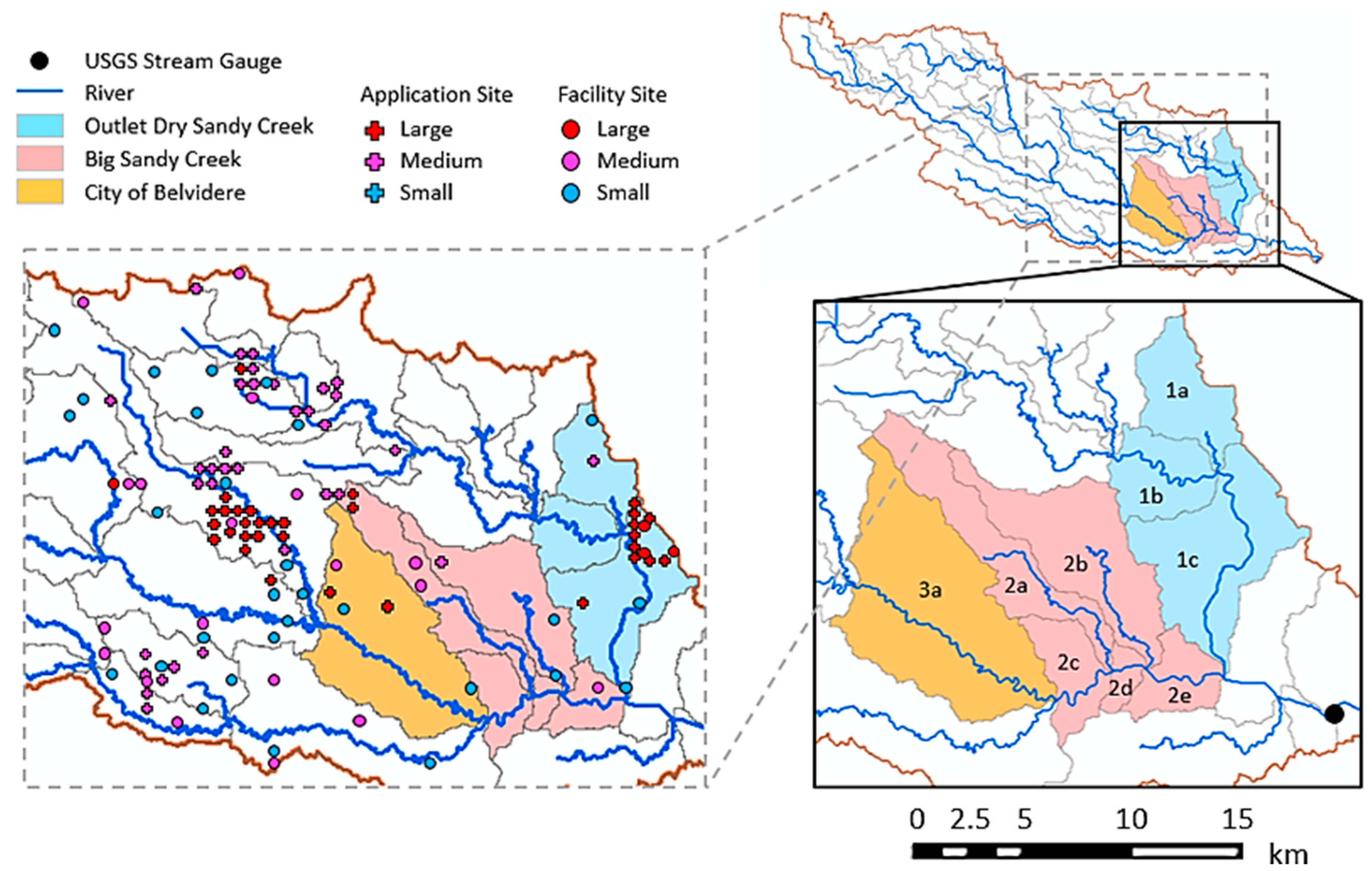
2.1. Study Area

The Big Sandy Creek Watershed (BSCW) is located along the northern edge of the Little Blue River watershed, Nebraska (Figure 1). The watershed is located between longitude 97°17′29′′ and 98°18′24′′ W and latitude 40°12′36′′ and 40°34′40′′ N. The area of BSCW is 1610 km² and the mean annual precipitation is 640 mm. Most of the precipitation occurs in the months of May, June and July. The climate is dry and continental, characterized by hot summers and cold winters. High winds, periodic droughts and flooding are climatic factors in this region. The land surface slopes from west-northwest to east-southeast with a maximum elevation of 1909 m to 1344 m above mean sea level. The topography is a relatively flat upland and slightly rolling hills, with narrow valley regions of low relief along rivers and streams. About 44% of the watershed has less than 3% slope, 29% has between 3–6% slope and the remaining 27% has more than 6% slope. The watershed lies within the Central Loess Plain Major Land Resource Area. Water-deposited sand and gravel occur as a heterogeneous mixture. Soils of the Jansen and Meadin series formed in loess overlaying the sand and gravel. Below is semi-consolidated bedrock or consolidated bedrock. The unconsolidated materials are primarily windblown clayey silts and loess overlying sands and gravels of alluvial origin. There are also alluvium soils that consist of valley sediments recently washed from the uplands and deposited on flood plains and stream terraces.

BSCW is predominantly an agricultural watershed with approximately 76% row crops (mainly corn and soybeans) and 23% pasture/hay. The remaining 1% includes urban, forest, water and other non-agricultural uses. Crop rotation primarily is corn and soybeans which accounts for 49% of the watershed while 27% is in rotation with at least two years of continuous corn. On average, approximately 15 km² of perennials crops such as alfalfa are grown annually.

The total area of the targeted sub-watersheds (Figure 2) is 240 km² and the mean annual precipitation is about 737 mm per year with approximately 80% coming as rain in high-intensity, convective thunderstorms. May and June are considered the critical erosion period following spring tillage and planting. Based on estimates from land use and crop rotation data for the target sub-watersheds, 49% of cropland is in a corn-soybean rotation and 36% is in a rotation with at least two years of continuous corn.

There are 19.2 km² of pasture in the target sub-watersheds. About 25,000 cattle (out of 36,000 in the whole BSCW) were in target sub-watershed 1a. Most pastures are used for summer grazing, but some are used for wintering cows prior to calving and staging pastures where cow-calf pairs are held after calving and prior to the summer pasture. Pastures often are overgrazed and void of vegetation along the streambanks. Moreover, cattle usually have direct access to the streams and they deposit fecal material while crossing, drinking from or loafing in the stream.

2.2. SWAT Model Set-Up

ArcSWAT (v2012) was used to divide the BSCW into 53 sub-watersheds, which were further divided into 1860 hydrologic response units (HRUs) based on the following thresholds: 5% land use, 0% soil and 0% slope. Each HRU was defined as a sub-watershed with similar land use, soil type and slope. Data used in SWAT model set-up/calibration/validation are presented in

Table 1. Input data used in the Soil and Water Assessment Tool (SWAT) setup and simulations.

Data Type	Date	Source	Description
Digital Elevation Model (DEM)	2014	United States Department of Agriculture—Natural Resources Conservation Service (USDA-NRCS)	10-m Resolution, Digital Elevation Model
Soils	2016	USDA-NRCS	State Soil Geographic (STATSGO)
Land use	2015	United States Department of Agriculture—National Agricultural Statistics Service (USDA-NASS)	National Agricultural Statistics Service—Cropland Data Layer
Weather	1989–2016	PRISM Climate Group	Daily precipitation, maximum and minimum daily temperature, solar radiation, wind speed, relative humidity
Crop & land management	2005	Nebraska Department of Environment and Energy (DEE), NRCS, UNL-CALMIT, Nebraska Department of Natural Resources (DNR)	Tillage operations, fertilizer and herbicide applications, crop rotation, time of planting, time of harvesting, irrigation, terraces
Streamflow Water quality	1989–2016 2002–2015	Nebraska DNR, Nebraska DEE	Flow measured at NDNR gauge 06883940 Nutrient concentration (total P, PO4, total N, NO2 + NO3), Atrazine and E. coli (2002 & 2012 data) at NDNR gauge 06883940

. The outlet of the BSCW was specified by a point downstream of the NDEE water quality monitoring station and the Nebraska Department of Natural Resources (DNR) streamflow gauging station 06883940 (latitude 40.235 and longitude −97.388). A lake at the US Meat Animal Research Center (Lake MARC) close to the headwater sub-watershed was included as a reservoir in the model though there is usually no outflow from this reservoir year round (Figure 1).

The NDEE provided monthly and/or bimonthly water-quality data on sediment (total suspended solids, n = 146), nitrogen (n = 146), phosphorus (n = 146), Atrazine (n = 105), and E. coli. (n = 39). Since daily data was not available for the water quality parameters, Load Estimator (LOADEST) was used to estimate daily loads for sediment, nutrients and Atrazine, while artificial neural network (ANN) was used to estimate daily E. coli concentrations. LOADEST estimates loads for a user-defined time period from discrete water quality samples and measured daily flow using a formulated regression model. Runkel et al. [34] provided detailed information on the LOADEST program and its techniques and methods. An ANN is a mathematical model comprising of a network of computation nodes with established connections between them [35]. Hsu et al. [36] and Sarle [37] provided detailed descriptions of ANN and its structure. An advantage of ANN is that it requires no a priori assumptions about the relationships between the independent and dependent variables as well as the mathematical functions to be used [38].

The prediction accuracy of an ANN model is strongly dependent of its generalization ability. A well-trained ANN model should have a very low root mean squared error at the end of the training and testing phases in order to avoid over-fitting and to generalize the model. An overfitted ANN model will give good predictions only for the training set (most of the time) but will perform poorly when predicting the test set (out-of-sample E. coli values). To develop the ANN model for predicting E. coli concentrations, the available dataset was randomly divided into a training dataset (70% of the total data), a validation dataset (15% of the total data), and a test dataset (15% of the total data). However, seeing that there were only thirty nine E. coli concentration observations for our study, the splitting of the dataset was done several times in order to get reasonable distributions for the training, validation, and test datasets which at least covered more than 80% of the range of E. coli values. This was an important step because any random split of our small E. coli dataset could give training, validation and test datasets with totally different data distributions based on the range of E. coli values covered. A model trained on a vastly different data distribution than the test set will perform inferiorly.

The fitting ANN was created using five hidden layers and Levenberg-Marquardt backpropagation algorithm in MATLAB (MathWorks Inc. Product R2019b). Training was done according to training parameters of the algorithm with their default values. Before ANN model development, the E. coli concentrations were log-transformed due to the presence of high concentration values. The initial predictor variables considered for predicting E. coli concentrations were cumulative precipitation on the day of sampling, cumulative precipitation a day before sampling, 7-day and 10-day moving averages of daily precipitation prior to sampling day, average streamflow on the day of sampling, and average streamflow a day before sampling. Later, the cumulative precipitation a day before sampling was removed due to low correlation with E. coli concentration. The coefficient of determination (R²) and root mean squared log error (RMSLE) statistics were used for checking model performance (Equations (1) and (2), respectively). RMSLE was used instead of root mean squared error (RMSE) because outliers can greatly increase the prediction error. While RMSLE considers only the relative error between predicted and actual values, and the scale of the prediction error is nullified by the log-transformation, in contrast, RMSE value increases in magnitude if the scale of error increases.

$$R^2=\frac{{\sum }_i{\left({\widehat{x}}_i-\overline{x}\right)}^2}{{\sum }_i{\left(x_i-\overline{x}\right)}^2}$$

(1)

$$RMSLE= \sqrt{\frac{1}{n}{\displaystyle \sum }_{i=1}^n{\left[\log (x_i+1)-\log \left({\widehat{x}}_i+1\right)\right]}^2}$$

(2)

where $x_i$ is the observed E. coli concentration (colony-forming unit (cfu)/100mL), ${\widehat{x}}_i$ is the predicted E. coli concentration (cfu/100 mL), $\overline{x}$ is the mean of the observed E. coli concentration (cfu/100 mL), and n is the total number of samples considered.

To improve modeling results and reduce the uncertainty in our SWAT model findings, management practices within the watershed were characterized. The management practices included the following: tillage operations, yearly planting and harvesting dates, nutrient and pesticide application rates and timing, irrigation and cattle density. Data on location of terraces and irrigation were also used in developing a detailed watershed model. Atrazine was simulated as loads from cropland only while E. coli was simulated as loads from both corn fields and pasture. Survey showed that producers commonly apply 1.7 kg/ha Atrazine to corn fields at a rate of 1.1 kg/ha at or before planting and 0.6 kg/ha post emergence. Management input files were created to simulate corn/soybeans rotation on all lands classified as soybeans in the land use layer file (Table S1 in Supplementary Materials). A grazing rate of 3.23 ha/cow was used for all pastures. SWAT was run at monthly time step from 1989 to 2016 with a warm-up period of five years (from January 1989 to December 1993).

2.3. Model Calibration and Validation

In order to parameterize the SWAT model to the given set of local conditions and to reduce uncertainty in model predictions, the auto-calibration program SWAT-CUP SUFI-2 was used to calibrate the model for streamflow, sediment, total nitrogen (TN), total phosphorus (TP), Atrazine and E. coli at the NDNR gauging station 06883940 with several repetitions of 1000 simulations. The SUFI-2 method takes into account all sources of uncertainties such as those from the input data, conceptual model, model parameters and observed data [39]. Manual calibration was also applied to improve the results of auto-calibration [40,41]. Before calibration, the ranges of targeted parameters for calibrating flow and pollutants were first defined by physically meaningful values. The values of these parameters were then allowed to change by replacement, addition, and relative change to the initial values. The model was calibrated (01/2004 to 12/2016) and validated (01/1994 to 12/2003) on a monthly time step using observed data at the NDRN gauging station 06883940. Streamflow was first calibrated, then sediment, nutrients, Atrazine and E. coli in that order.

In order to ensure a good calibration procedure, we used multiple statistics, each covering a different aspect of the hydrograph, so that the whole hydrograph is covered [42]. This reduced the unnecessary emphasis that using a single statistic can place on matching one aspect of the hydrograph at the expense of other aspects while recognizing potential errors in the observed data [43]. The model performance was assessed using R², Nash-Sutcliffe efficiency (NS), root mean square error (RMSE)-observations standard deviation ratio (RSR), and percent bias (PBIAS) as recommended by Moriasi et al. [42]. These statistics were calculated using Equations (1) and (3)–(5) respectively. R² values range from 0 to 1 and higher values indicate a better fit of the simulated data to the observed data. According to the general performance ratings for statistics for a monthly time step recommended by Moriasi et al. [42], values of R² > 0.5 are considered satisfactory. NSE ranges from −∞ to 1, where a value of 1 indicates an optimal model fit to the observed data. An NSE value between 0.75 and 1 shows a very good model fit, 0.65–0.75 is good, 0.50–0.65 is satisfactory, and <0.5 is considered unsatisfactory. RSR standardizes the RMSE with the standard deviation of the observed data. This ranges from 0 to large positive values with lower values indicating better model fit. RSR values between 0 and 0.5 indicate a very good model fit, 0.5–0.6 is good, 0.60–0.7 is satisfactory, and >0.7 is unsatisfactory. PBIAS is used to assess the average tendency of simulation to over- or under-predict the observation data. The optimal value of PBIAS is 0, with low values indicating better model fit. For streamflow, sediment, and nutrients, absolute PBIAS values <10%, <15%, and <25% respectively indicate a very good model fit, 10–15%, 15–30%, and 25–40% indicate good, 15–25%, 30–55%, and 40–70% indicate satisfactory, and >25%, >55%, and >70% indicate unsatisfactory. Positive PBIAS values show the model is underestimating bias while negative values indicate bias overestimation [44]. Visual comparisons between observed and simulated graphs were also carried out in addition to the statistics to see how peaks aligned in both observation and simulation.

$$NSE=1- \left[\frac{{\sum }_{i=1}^n{\left(X_i^{obs}-X_i^{sim}\right)}^2}{{\sum }_{i=1}^n{\left(X_i^{obs}-X^{mean}\right)}^2}\right]$$

(3)

$$RSR=\frac{RMSE}{{STDEV}_{obs}}=\frac{\left[\sqrt{{\sum }_{i=1}^n{\left(X_i^{obs}-X_i^{sim}\right)}^2}\right]}{\left[\sqrt{{\sum }_{i=1}^n{\left(X_i^{obs}-X^{mean}\right)}^2}\right]}$$

(4)

$$PBIAS=\left[\frac{{\sum }_{i=1}^n\left(X_i^{obs}-X_i^{sim}\right)\times 100}{{\sum }_{i=1}^n\left(X_i^{obs}\right)}\right]$$

(5)

where $X_i^{obs}$ is the observed variable (streamflow or pollutant load), $X_i^{sim}$ is the simulated variable, $X^{mean}$ is the mean of $n$ variables, ${STDEV}_{obs}$ is the standard deviation of observations, and $n$ is the number of observations.

2.4. Implementing BMPs in Hotspots

Hotspots for prioritizing installation of BMPs to reduce sediment, nutrients, Atrazine and E. coli runoff were identified from data collected during BSCW windshield surveys as well as data obtained from Agricultural Conservation Planning Framework (ACPF) and Agronomy technical notes. Although several potential BMPs were highlighted in the NWQI project, this study focused on six BMPs. These BMPs include no-till farming practice (NT), filter strip (FS), crop rotation (CR), grassed waterway (GW), terrace (TR), and reduced Atrazine application rate (RAR). The calibrated and validated SWAT model was used to evaluate the BMPs in terms of their effectiveness in reducing pollutant loads. Slope, soil type, and crop type were considered major factors in implementing the BMPs since these factors could influence pollutant runoff under normal farming and grazing operations.

The expected load reductions from BMPs as well as the total areas considered by the NWQI project for implementation of these BMPs in three years are shown in

Table 2. Pollutant load and concentration reduction goals from target sub-watersheds.

Pollutant	Location	Pollutant Reduction Goal
Sediment	Target sub-watersheds	20%
Total Nitrogen	Target sub-watersheds	20%
Total Phosphorus	Target sub-watersheds	20%
Atrazine	gauging station 06883940	12 µg/L
E. coli	gauging station 06883940	112 cfu/100 mL

and

Table 3. Areas (km²) considered for implementation of best management practices (BMPs) in three years.

BMP	Total Area	Year 1	Year 2	Year 3
NT	10.12	2.02	4.05	4.05
CR	2.02	0.40	0.81	0.81
FS	2.02	0.40	0.81	0.81
GW	2.02	0.40	0.81	0.81
TR	0.80	0.16	0.32	0.32
RAR	44.52	8.90	17.81	17.81

respectively. The load reductions for sediment, nitrogen and phosphorus are for the targeted subbasins (Figure 2) while the target concentrations of E. coli and atrazine are for the Nebraska Department gauging station. Pollutant loads were simulated before and after the implementation of BMPs. The locations and type of BMPs were based on the data provided by the NWQI project. Although the configurations of the BMPs may be variable in the real world, we assumed that they were generally representative and were meant to reflect the general operations of the BMPs in the target sub-watersheds in BSCW (

Table 4. BMPs in target sub-watersheds and representation in SWAT.

BMP	Management Practice	Representation in SWAT
NT	No-till	Field cultivator and tandem disk plow replaced with no-tillage operation in corn years (in rain fed and irrigated continuous corn and corn/soybeans rotation) and in soybean years (in rain fed and irrigated corn/soybeans rotation); mixing efficiency of tillage operation (EFFMIX) = 0.05; depth of mixing caused by tillage operation (DEPTIL) = 25 mm; SCS runoff curve number for moisture condition II (CNOP) reduced by 5%
CR	Crop rotation	Continuous corn replaced with corn/soybeans
FS	Filter strip	Used recommendations at optimal conditions on slopes greater than 6%: fraction of total runoff from the entire field entering the most concentrated 10% of the vegetative filter strip (VFSCON) = 0.5; field area to vegetative filter strip area ratio (VFSRATIO) = 40; fraction of flow through the most concentrated 10% of the vegetative filter strip that is fully channelized (VFSCH) = 0
GW	Grassed waterways	Used recommendations: Manning’s n value for the main channel (CH_N2) = 0.3 at optimal conditions; channel cover factor (CH_COV2) = 0.001 for fully protected channels; channel erodibility factor (CH_COV1) = 0.001 for zero erodibility
TR	Terrace	Used on slopes greater than 6%: Curve number reduced by 5 units; Universal Soil Loss Equation Practice factor (USLE_P) modified by multiplying with the suggested values given in Section 2.4.
RAR	Reduced Atrazine application rate	Application rates in corn reduced by 50%

).

NT increases the amount of residue on soil surface after crop harvest and before planting the next crop. To represent no-till farming in the SWAT model, conventional tillage operations with field cultivators and tandem disk plows were replaced with no tillage by modifying the till.dat and management files (Table 4). Crop rotation switched the conventional continuous corn to the two-year corn-soybean rotation (Table S1 in Supplementary Materials). According to the SWAT conservation practice modeling guide [45], representing filter strip in SWAT included adjusting the fraction of total runoff from a field entering the most concentrated 10% of a filter strip (VFSCON), field area to filter strip area ratio (VFSRATIO), and the fraction of flow within the most concentrated 10% of the filter strip that is fully channelized (VFSCH). Grassed waterway was represented by adjusting channel Manning’s roughness (CH_N2), channel cover factor (CH_COV2) and the channel erodibility factor (CH_COV1) [46,47,48]. Terrace was simulated by modifying the runoff curve numbers of cropland according to Strauch et al. [49] and modifying the Universal Soil Loss Equation practice factor (USLE_P) by using the values 0.12 (for slopes <3% and >6%) and 0.10 (for slopes between 3% and 6%) according to Haan et al. [50]. RAR was simulated by reducing Atrazine application rate by 50% in both rainfed and irrigated continuous corn and corn/soybean rotation.

It is important to note that whenever an empirical approach is used for simulating BMPs, it usually involves applying a linear approach to non-linear problems. In reality, due to the reason that one cannot expect any ratio or factor to be time-invariant irrespective of the hydro-meteorological, soil or land cover conditions, the results of BMP simulations and the direct comparisons amongst BMPs (in terms of pollutant reduction criteria) should be interpreted with caution.

Changes in the amount of sediment, TN and TP were evaluated at the outlets of the target sub-watersheds while changes in Atrazine and E. coli loads were evaluated at the NDNR gauging station 06883940 according to the NWQI project plan. The changes in pollutant loads due to BMPs’ implementation were compared with the baseline scenario which is the current practice carried out in the watershed. The baseline scenario was established with the calibrated SWAT model. The percent change was calculated using Equation (6):

$$Percent change= \left(\frac{Loa{d}_f-Loa{d}_i}{Loa{d}_i}\right)\times 100$$

(6)

where $Loa{d}_i$ is the load before implementing BMP and $Loa{d}_f$ is the load after implementing BMP (negative values imply reduction).

3. Results and Discussion

3.1. Daily E. coli Load Prediction

This study used ANN to predict daily E. coli concentrations at the gauging station. Figures S1 and S2 in the Supplementary Materials show the performance of the ANN model for training, validation and testing. The blue, green and red bars in Figure S1 (left) represent the training data, the validation data, and the testing data, respectively. The error from the neural network ranged from −0.52 logcfu/100 mL (leftmost bin) to 0.85 logcfu/100 mL (rightmost bin). The test set error and the validation set error had similar characteristics, and no significant overfitting occurred after iteration 3 where the best validation performance occurred (Figure S1 right). The training stopped when the validation error increased for six validation checks, which occurred at epoch 9. The RMSLE values for training, validation and testing at iteration 3 were all less than 0.45 (MSLE < 0.2) with an overall R² value of 0.83 (Figure S2).

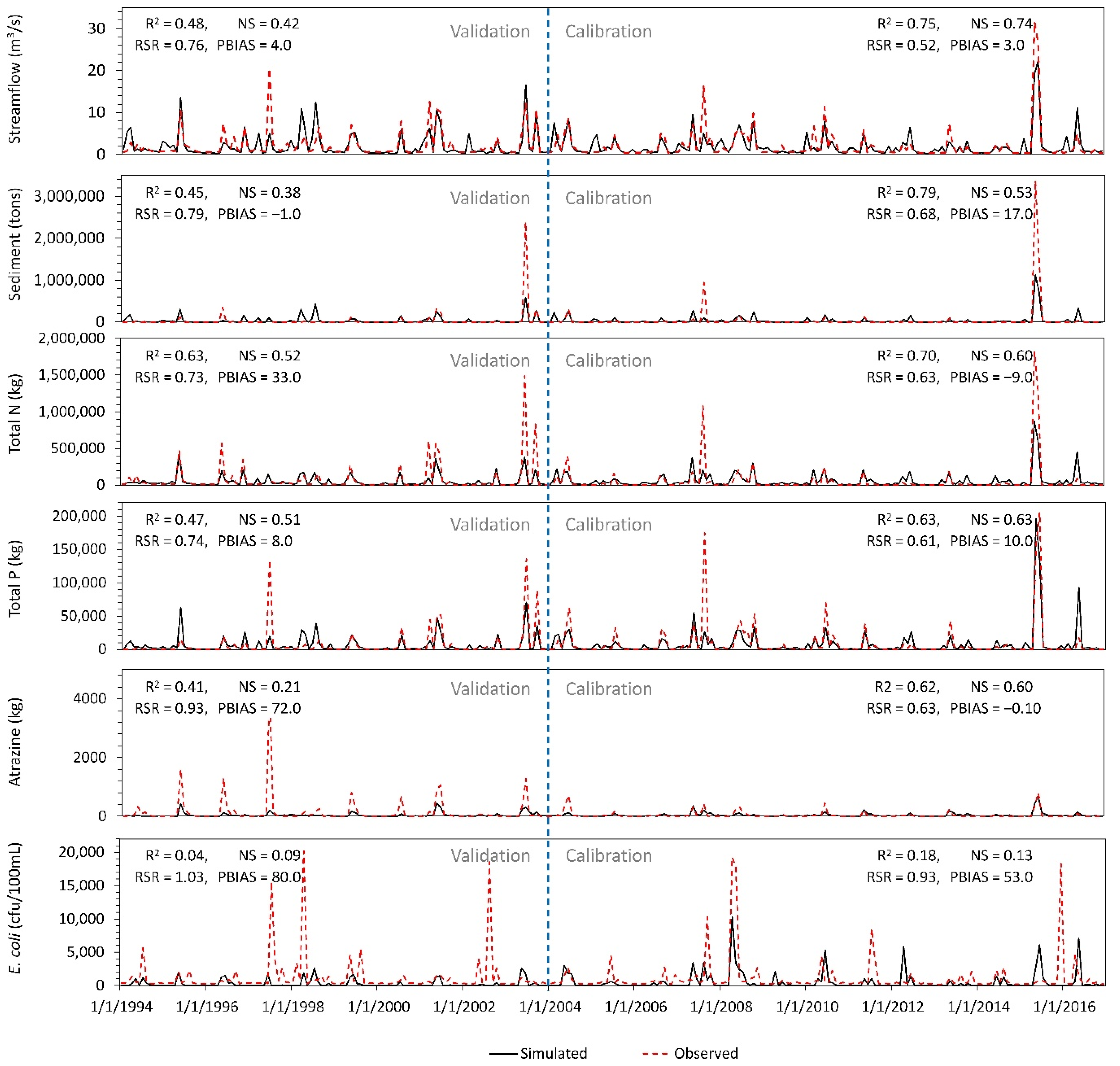
3.2. Streamflow and Water Quality Simulation

Table S2 in the Supplementary Materials lists the parameters for SWAT model calibration of streamflow and pollutants in the BSCW. The default values of these parameters were extracted from SWAT documents and used to set the initial parameter ranges. The SWAT–CUP program with the SUFI–2 algorithm was used for calibrating the model on monthly time step with 1000 runs. Figure 3 graphically illustrates the observed and simulated streamflow, sediment loss, TN loss, TP loss, Atrazine loss and E. coli at the NDNR gauging station 06883940. Based on the good R², NSE, RSR and PBIAS agreements between monthly observed and simulated flow, sediment, nutrients and Atrazine for the calibration period 2004–2016, the results showed that the model successfully predicted these variables in the study watershed (Figure 3). For streamflow, the NSE, RSR and PBIAS values were 0.74, 0.52, and 3.0, respectively. Furthermore, the performance of the calibrated model was close to satisfactory level for the validation period 1994–2003 with NSE  =  0.42 and PBIAS = 4.0 indicating the ability of the model to represent various climatic conditions (Figure 3).

Simulated sediment loss was also compared with the observed values at the gauging station. The calibration and validation results also showed good agreement between simulations and observations with acceptable statistical criteria (NSE  =  0.53, RSR = 0.68, PBIAS = 17.0). Similarly for TN and TP, the calibration and validation results indicated good performance of the model. The calibration and result for Atrazine indicated good performance although the validation objective functions are slightly below the satisfaction levels. The poor E. coli calibration and validation results were probably due to the uncertainty involved in E. coli source estimation from wildlife and wastewater treatment facilities, coupled with exclusion of failing septic systems in our SWAT model. A satisfactory calibration and validation result may be achieved if detailed wildlife records, which include daily information on forage type, number and type of swine and sheep, number and type of cattle grazing, the number of days each group stayed in each pasture or feedlot for the entire study period, unrestricted cattle access to streams, the number of migrating birds, etc., were considered as model inputs.

In general, the underestimation of LOADEST peaks by our SWAT model (Figure 3) may be attributed to poor LOADEST estimates due to the unavailability of water quality data from major storm events. In a study focused on simulating sediment and nutrient loads in several gauging stations, Park and Engel [51] observed that, although regression models based on LOADEST simulated pollutant loads reasonably with reliable model coefficients, some of their results also indicated that LOADEST overestimated pollutant loads and had a bias. With nine sub-sampled water quality data sets, they observed that some regression models in LOADEST overestimated sediment load by more than ten times and overestimated nitrogen and phosphorus loads by several hundred times. However, estimates of all pollutants significantly improved with the inclusion of water quality data for maximum streamflow. Therefore they concluded that avoiding water quality data extrapolation, coupled with the availability of water quality data from storm events, were critical in annual pollutant load estimation using LOADEST.

Moreover, the underestimation of some peaks for the five pollutant loads (Figure 3) could be dependent on whether the SWAT inputs such as weather (especially precipitation) and management operations (fertilizer type, application timing, application amount, and application location) which vary spatially and temporally were true representations of reality in the watershed. For instance, regardless of how complex or detailed a model is in simulating hydrological processes, the accurate representation of precipitation over the watershed (and sub-watersheds) is important for accurate runoff and pollutant load simulation. Since SWAT uses the minimum distance from a sub-watershed centroid to the available weather stations for selecting its representative station, the PRISM weather data used in our study may not be totally representative of the reality in the sub-watersheds of BSCW. This could also have contributed to the underestimation of simulated peaks. Furthermore, in order to reduce the errors involved in predicting E. coli concentration using data-driven methods, a recent study by Abimbola et al. [52] showed that more detailed information about animal management (e.g., animal density, locations or distances from streams, and grazing patterns) needs to be coupled with hydro-meteorological variables.

Another potential reason for underestimating the pollutant loads for some storm events is the overflowing of the reservoir. The reservoir, located in the headwaters of Big Sandy Creek, has high E. coli and nutrient concentrations [53]. From a separate study, we observed that the reservoir overflowed in 2019, but there is no documentation of previous reservoir water depths and overflowing.

3.3. Effect of Individual BMP Scenarios

This study evaluated the performance of five individual BMPs using the ‘best-case’ scenarios where the BMPs were implemented individually over the entire target sub-watersheds. The plan of the NWQI project is to implement all or combinations of these BMPs on portions of the target sub-watersheds for three years (Table 3). However, since there were many uncertainties in the future adoption of theses BMPs by agricultural producers, this made it difficult to select the exact future locations of the BMPs in the target sub-watersheds. Thus, the ‘best-case’ scenarios were based on the total areas of the target sub-watersheds, and the reductions of these ‘best-case’ scenarios were later scaled down to estimate reductions based on the acreage proposed by NWQI (Table 3). The effectiveness of the BMPs in mitigating sediment loss, total N loss, total P loss, Atrazine loss, and E. coli loss was determined under baseline climate conditions (2004–2016, calibrated). This baseline scenario formed the basis for evaluating the individual BMP scenarios. The differences in average annual losses of pollutants associated with BMP implementation were computed for the calibration period and aggregated by BMP. Summaries of the long-term average annual percentage reductions at the target sub-watersheds and gauging station are presented in

Table 5. Average annual reduction (standard deviation) in loadings using no-till at the target sub-watersheds. Negative values indicate an increase.

Sub-Watershed	Annual Reductions (%)
	Sediment	Total N	Total P
1a	23 (21)	7 (8)	16 (10)
1b	22 (18)	−8 (9)	6 (7)
1c	19 (12)	1 (3)	7 (3)
2a	39 (7)	−2 (2)	4 (2)
2b	22 (17)	−6 (5)	−1 (5)
2c	20 (10)	−3 (3)	1 (2)
2d	19 (7)	−2 (1)	1 (1)
2e	17 (8)	−2 (2)	0 (1)
3a	37 (17)	−1 (3)	8 (6)

,

Table 6. Average annual reduction (standard deviation) in loadings using crop rotation at the target sub-watersheds. Negative values indicate an increase.

Sub-Watershed	Annual Reductions (%)
	Sediment	Total N	Total P
1a	−1 (4)	23 (12)	22 (9)
1b	3 (7)	−5 (4)	11 (5)
1c	1 (3)	7 (6)	11 (6)
2a	1 (3)	−1 (2)	1 (1)
2b	0 (3)	−1 (1)	2 (1)
2c	0 (4)	−1 (2)	3 (2)
2d	−2 (5)	0 (2)	2 (2)
2e	−1 (3)	0 (1)	1 (1)
3a	5 (9)	−3 (3)	5 (2)

,

Table 7. Average annual reduction (standard deviation) in loadings using filter strips at the target sub-watersheds. Negative values indicate an increase.

Sub-Watershed	Annual Reductions (%)
	Sediment	Total N	Total P
1a	14 (13)	15 (8)	15 (9)
1b	17 (14)	18 (7)	18 (9)
1c	19 (12)	23 (10)	24 (11)
2a	29 (11)	24 (10)	27 (11)
2b	20 (12)	27 (9)	28 (10)
2c	21 (12)	23 (9)	25 (10)
2d	21 (11)	23 (10)	25 (11)
2e	20 (12)	23 (10)	25 (11)
3a	27 (10)	21 (7)	25 (7)

,

Table 8. Average annual reduction (standard deviation) in loadings using grassed waterway at the target sub-watersheds. Negative values indicate an increase.

Sub-Watershed	Annual Reductions (%)
	Sediment	Total N	Total P
1a	99 (4)	78 (16)	85 (15)
1b	99 (6)	59 (20)	80 (24)
1c	97 (15)	56 (23)	69 (24)
2a	95 (11)	46 (17)	54 (19)
2b	97 (13)	55 (18)	64 (21)
2c	94 (20)	46 (20)	56 (23)
2d	91 (26)	43 (20)	50 (23)
2e	93 (23)	44 (20)	52 (23)
3a	97 (6)	49 (16)	61 (18)

and

Table 9. Average annual reduction (standard deviation) in loadings using terrace at the target sub-watersheds. Negative values indicate an increase.

Sub-Watershed	Annual Reductions (%)
	Sediment	Total N	Total P
1a	72 (11)	51 (16)	58 (15)
1b	77 (9)	22 (10)	49 (19)
1c	61 (15)	14 (8)	28 (13)
2a	76 (11)	5 (4)	16 (9)
2b	73 (11)	4 (4)	18 (10)
2c	62 (16)	3 (3)	14 (9)
2d	51 (19)	1 (1)	8 (6)
2e	46 (17)	1 (2)	8 (5)
3a	77 (17)	15 (8)	29 (11)

. The distributions of annual reductions (box plots) and intra-annual reductions (bar charts) at the target sub-watersheds are shown in the Supplementary Materials (Figures S5–S16).

3.3.1. No-Tillage Scenario

When compared to the existing baseline conditions, results showed that change of tillage practices (e.g., field cultivator, tandem disk) to no-till resulted in sediment load reductions in all the hotspots (target sub-watersheds) and total phosphorus load reductions in most of the hotspots. Reductions in sediment and total phosphorus loads at sub-watershed level ranged from 17% to 39% and 1% to 16% respectively, with little or no increase in total phosphorus loads in two sub-watersheds (Table 5). Distributions of annual and intra-annual reductions are shown in the Supplementary Materials. In general, the reduction in sediment and total phosphorus loads with no-till could be due to the lower mixing efficiency (0.05) and lower mixing depth (~25 mm) of the no-till when compared with field cultivator (mixing efficiency = 0.3; depth of mixing 100 mm) and tandem-disk regular (mixing efficiency = 0.6; depth of mixing = 75 mm) in SWAT modeling. No-till results in no disturbance of the soil through tillage, and leaves previous crop residue on the soil surface. This reduces soil erosion due to surface runoff, especially during the early part of the growing season when fields are bare and more likely to be eroded [54]. Similar to our study, several SWAT studies have shown percentage reductions in sediment and total phosphorus due to the application of no-till at watershed scale [55,56,57].

Similar to some SWAT studies showing mixed results on the effects of no-till on total nitrogen and nitrate in literature [55,58,59], our no-till BMP predicted slight load reductions in only two sub-watersheds while other sub-watersheds had slight increase in loads. Mittelstet et al. [59] also found increase in simulated nitrate loads for three hydrologic soil groups in some Nebraska watersheds. In our study, the relatively high reductions in total nitrogen and total phosphorus loads in sub=watershed 1a was because this sub-watershed had feedlots with about 25,000 cattle.

3.3.2. Crop Rotation Scenario

Table 6 shows sediment and nutrient losses from crop rotation in the target sub-watersheds. In this scenario analysis, results showed that sediment was not sensitive to crop rotation management with values ranging between −2% and 5%. In a previous study focusing on crop rotation scenarios which included continuous corn, continuous soybean, and corn-soybean rotation in Mississippi, Ni and Parajuli [60] also reported similar insensitivity of sediment to crop rotation.

The total nitrogen loss would be expected to be lower in the corn-soybean rotation BMP than that in the continuous corn baseline due to the lower amount of nitrogen fertilizer application rate to soybeans. However, since the baseline land use in all of the target sub-watersheds contained about two times more corn-soybean rotation than continuous corn on the average, the conversion of continuous corn to corn-soybean rotation showed little effect in total nitrogen loads with mixed results. In addition, because total nitrogen uptake by corn and soybean may be similar [61,62], the only difference between the total nitrogen load reductions for sub-watershed 1a and other hotspots was probably due to the large number of cattle in feedlots present in sub-watershed 1a.

For total phosphorus loads, there were different magnitudes of reductions in all hotspots in the corn-soybean rotation scenario (Table 6). Compared to sub-watershed 1a (22% reduction), relatively lower total phosphorus reductions (11%) occurred in sub-watersheds 1b and 1c, and small reductions (between 1 and 5%) in the remaining hotspots. The 1–5% reductions in these hotspots could be attributed to the differences in cropland and pasture areas, as well as areas with slopes greater than 6%. In the baseline scenario, hotspots with small pasture areas (<22%) had more corn-soybean rotation (>53%) than continuous corn (<23%), which resulted in small reductions when continuous corn was converted to corn-soybean rotation. On the other hand, since hotspots with larger areas with >6% slope had pasture on these slopes close to the streams (see land use map for the inset in Figure S3 in Supplementary Materials), we could only speculate that the total phosphorus slightly reduced, probably because of phosphorus trapping and/or lower fertilizer demand in corn-soybean rotation. Distributions of annual and intra-annual reductions are shown in the Supplementary Materials.

3.3.3. Filter Strip Scenario

High reductions in sediment and nutrient loads were achieved by implementing filter strips in the agricultural areas on slopes greater than 6% (Table 7). Under this BMP, the highest reduction in pollutants was observed for total phosphorus with an average of 23.5%, followed by total nitrogen with an average of 20%. The higher reduction for total phosphorus may be caused by differences among nutrient sources considered in this study. Moreover, reductions were slightly higher in hotspots with less than 20% pasture (sub-watersheds 2a and 2b) than for those with pasture areas greater than 20% since most of the pastures were on slopes greater than 3% in most of the hotspots in the baseline scenario. Distributions of annual and intra-annual reductions are shown in the Supplementary Materials.

A number of studies have reported high removal rates of sediment and nutrients in surface flows through the use of filter strips [63,64]. In their study conducted in Iran, Babaei et al. [63] found filter strip to be a very effective BMP in reducing total nitrogen load (42.61%), and total phosphorus load (39.57%). In a field-scale modeling conducted by Merriman et al. [64], their results indicated that constructing filter strips was an effective BMP for reducing sediment (97% reduction), total nitrogen (13%) and total phosphorus (63%) loads.

3.3.4. Grassed Waterway Scenario

The highest reductions in pollution loads were achieved by implementing grassed waterways in the hotspots (Table 8). Under this BMP, the highest reduction in pollutants was observed for sediment (>91%). These high reductions were due to fact that the target hotspots already had pastures on slopes greater than 6% and close to stream reaches in the baseline scenario (Figures S3 and S4 in the Supplementary Materials). These pastures acted as filter strips. Coupling the existence of pastures with the implementation of grassed waterways in all tributaries in the hotspots, such high reductions would be expected. Furthermore, the results indicated that the total phosphorus loads were reduced slightly more than the total nitrogen (Table 8). Distributions of annual and intra-annual reductions are shown in the Supplementary Materials. Merriman et al. [64] observed reductions of 60%, 9% and 39% for sediment, total nitrogen and total phosphorus loads, respectively, with grassed waterways. When they combined grassed waterways with filter strips, they observed load reductions of 99%, 9% and 64% for sediment, total nitrogen and total phosphorus, respectively.

3.3.5. Terrace Scenario

Constructing terraces across field slopes would be an effective BMP for reducing erosion in any watershed. SWAT predicted that terraces, if constructed across slopes greater than 6% in hotspots, would reduce annual sediment, total nitrogen, and total phosphorus loads by 46–77%, 1–51% and 8–58%, respectively (Table 9). Although sub-watersheds 2d and 2e both had more than 60% land areas with slopes >6%, when compared to the other seven hotspots with an average of 41% area and slopes >6% (slope area in all nine hotspots ranging from 25.8% to 53.7%), the relatively lower reductions in sediment and nutrients in sub-watersheds 2d and 2e could be attributed to the bigger pasture areas that already existed on these slopes in the baseline scenario. With >6% slope area in all nine hotspots ranging from 25.8% to 53.7%, sub-watersheds 2a and 2b had an average of 33%, slightly above sub-watershed 1a (25.8%). Moreover, both sub-watersheds also had more land areas (average of 37.8%) with slopes <3% compared to other hotspots (average of 23.5%). For these two hotspots, terrace was not so effective probably because there was not enough slope gradient. The dominant flow process in both hotspots was most likely saturation excess overland flow because the field areas were relatively flat. In a field study in southwestern Iowa, Gassman et al. [65] found ten-fold reductions in sediment and nutrients loads with terrace BMP.

3.3.6. Atrazine Concentration at Gauging Station

Results indicated that reducing the application rates of Atrazine to 50% on all rainfed and irrigated corn in the ‘best-case’ scenario only reduced Atrazine concentration by 21% (from 92 µg/L to 72 µg/L) at the NDNR gauging station 06883940. This reduced concentration was still six times higher than the target concentration of 12 µg/L. As shown in Figure 4, baseline Atrazine concentrations in the reaches of sub-watersheds 2a and 2b were three times higher compared to other hotspot reaches. This was because sub-watersheds 2a and 2b were headwater sub-watersheds (Figure 2), and they had the highest combined percent of continuous corn and corn-soybean, 80.2% and 79.6%, respectively. Thus, the effect of dilution was minimal in both reaches. Since the predominant land use types in BSCW are corn-soybeans and continuous corn (Figure S3), there is a need to reduce Atrazine application in several upland sub-watersheds. With respect to the nine hotspots, there is need for more application rate reductions in sub-watersheds 2a and 2b, while in the BSCW in general, reducing or eliminating the use of Atrazine may be the way forward in order to achieve the target concentration.

Weed management alternatives to Atrazine should also be promoted for adoption in the BSCW. In field trials in major sweet corn production areas which included three US states, Arslan et al. [66] demonstrated that Atrazine-free weed management systems were comparable in performance to standard Atrazine-containing weed management systems based on input from sweet corn farmers. These systems included treatments with tembotrione either with or without interrow cultivation, and treatments with topramezone in locations where small-seeded weed species were prevalent. A published meta-analysis of existing literature by Rohr and McCoy [67] and other studies [68,69,70,71,72] showed the effects of different concentrations of Atrazine on amphibians and freshwater fish, which led to the conclusion that the adverse effects of Atrazine must be weighed against any of its benefits. It is important to note that whereas the European Union (EU) announced a ban on using Atrazine in 2003 because of unpreventable water contamination, the US Environmental Protection Agency (EPA) approved the continued use of Atrazine that same year [73].

3.3.7. E. coli Concentration at Gauging Station

Although grassed waterway had the highest E. coli reduction of 64%, followed by crop rotation (29% reduction), none of the BMPs reduced the E. coli concentrations at the gauging station to the target concentration of 112 cfu/100 mL (Figure 5). Other BMPs had less than 10% reductions. Even though the reach of sub-watershed 1a had very high average E. coli concentration because of the feedlots with about 25,000 cattle, this high concentration was diluted by streamflow from upland reaches flowing through reach 1b and continuing downstream to reach 1c (Figure 2). However, this dilution was not sufficient to reduce the concentration to target value. Moreover, the relatively high E. coli concentration in reach 2c did not originate from reach 3a. Rather, it was due to high concentrated streamflow from upland reaches with feedlots combining with streamflow from reach 3a before going through reach 2c (Figure 2).

Due to the uncertainty involved in E. coli source estimation from wildlife, coupled with exclusion of failing septic systems in our SWAT model, an effective manure management plan needs to be put in place based on the application amount, timing, and strategy, most especially in sub-watersheds with the greatest E. coli source contribution. This would go a long way to further reduce E. coli concentration at the gauging station to the target value. The target value can also be met by repairing failing septic tanks.

3.4. Scaling down the Best-Case Scenario BMPs

In order to examine how the BMPs would perform based on the control areas considered by the NWQI for their implementation in three years, we aggregated the nine hotspots to reflect the three major hotspots in the NWQI plan. Hotspots with numbers 1-, 2- and 3- in Figure 2 correspond to the three target sub-watersheds delineated by US Geological Survey (USGS) 12-digit hydrologic code (HUC-12). These target sub-watersheds 1, 2 and 3 are Outlet Dry Sandy Creek, Big Sandy Creek, and City of Belvidere, respectively. The aggregated reductions in these three HUC-12 sub-watersheds were calculated using the weighted average of the contributing hotspot areas. The load reductions were scaled down based on an area ratio method. Although there may not be linear relationships between increasing BMP implementation scale and Atrazine or E. coli concentration reductions at the gauging station due to the contributions from other 44 sub-watersheds, a linear relationship in the form of area ratio may be useful for sediment and nutrient loads transported with water into a reach at sub-watershed scale.

The area ratio method used in this study is similar to the drainage-area ratio method commonly used for estimating streamflow for ungauged sites. It was based on the assumption that the reduction in load for a hotspot of interest could be estimated by multiplying the ratio of the BMP implementation area for the hotspot of interest and the BMP area for the ‘best-case’ scenario in that hotspot by the load reduction for the ‘best-case’ scenario. To simplify the evaluation and to ensure that the estimated load reduction was an unbiased estimate of the order of magnitude of the actual load reduction, the average load reduction for the calibrated years was used rather than load reductions for individual months. It is important to note that while this area ratio method may overestimate or underestimate loads for some hotspots, it is a simple method that may be sufficient to capture the order of magnitude of load reductions. To remove all uncertainties and correct the bias in load estimations due to area ratio, a BMP simulation in SWAT would require having all the information and details about the exactness of all input parameters, including specific locations of each BMP, timing, proportion, magnitude, and adoption of the BMP by farmers.

However, with the exception of filter strip, no individual BMP was effective in achieving the targeted load reductions after down-scaling the implementation acreage (

Table 10. Scaled-down load reductions from BMPs in the three HUC-12 sub-watersheds aggregated from the nine hotspots.

BMP	Aggregated Subwatershed	Best-Case Annual Reduction (%)			Scaled Annual Reduction (%)
		Sediment	Total N	Total P	Sediment	Total N	Total P
NT	1	20.7	0.5	9.0	1.3	0.0	0.6
	2	26.0	−3.7	1.0	1.3	−0.2	0.0
	3	37.0	−1.0	8.0	2.4	−0.1	0.5
CR	1	1.0	8.3	13.7	0.0	0.3	0.5
	2	0.1	−0.8	1.7	0.0	0.0	0.1
	3	5.0	−3.0	5.0	0.2	−0.1	0.2
FS	1	17.3	19.9	20.4	13.7	15.7	16.2
	2	22.9	24.9	26.8	15.9	17.3	18.7
	3	27.0	21.0	25.0	24.6	19.1	22.7
GW	1	97.9	61.6	75.4	6.6	4.1	5.1
	2	95.2	49.2	57.8	6.4	3.3	3.9
	3	97.0	49.0	61.0	6.5	3.3	4.1
TR	1	67.3	24.9	40.1	0.5	0.2	0.3
	2	68.0	3.7	15.2	0.5	0.0	0.1
	3	77.0	15.0	29.0	0.7	0.1	0.3
Grand Total	1				22.2	20.4	22.6
	2				24.1	20.5	22.8
	3				34.4	22.3	27.8

). Therefore, to achieve a 20% sediment and nutrient load reduction in the hotspots, we suggested that multiple BMPs be implemented. Overall, a combination of filter strip, grassed waterway and Atrazine rate reduction is most likely to yield measureable improvement both in the hotspots and at the gauging station.

4. Conclusions

With limited funding and acreage for BMP implementation, the NWQI has set a target of 20% reduction in sediment and nutrients losses from target sub-watersheds (hotspots) in three years. With the focus of the NWQI in these hotspots, our results indicated that individual conservation practices were effective in reducing a particular pollutant load when implemented all over the hotspots (best-case scenario). Among the BMPs modeled, grassed waterway was the most effective individual BMP in reducing sediment and nutrient loads in the hotspots, and reducing E. coli concentrations at the gauging station. Reducing application rate by 50% was most effective for Atrazine reduction at the gauging station. It is noteworthy that, even in the best-case scenario, Atrazine and E. coli target concentrations at the station were not met. Besides the hotspots, a reduction or elimination of Atrazine use in upland sub-watersheds, and treatment of manure in sub-watersheds with high number of animals and feedlots, would benefit the whole BSCW.

When implementation areas were scaled down, a combination of filter strip and grassed waterway was sufficient for meeting the 20% reduction target for sediment and nutrients. In general, a combination of BMPs could yield measureable improvement in the hotspots and at the gauging station. Implementing a BMP such as filter strip may require additional management effort from farmers, and may reduce yields and profits due to high operating costs, especially in the first few years of adoption while the farmers are still learning how to successfully implement it. In addition, BMPs such as filter strips which displace cropland may create high opportunity costs for agricultural producers since there will not be profits on the plots of land with filter strips.

Moreover, future work needs to consider how to achieve these reduction objectives by exploring barriers to, and incentives for adopting and implementing the BMPs so that BMP solutions meet the target needs going forward.

References

1. Carkovic, A.B.; Pastén, P.; Bonilla, C.A. Sediment composition for the assessment of water erosion and nonpoint source pollution in natural and fire-affected landscapes. Sci. Total Environ. 2015, 512, 26–35. [Google Scholar] [CrossRef]
2. Shen, Z.; Liao, Q.; Hong, Q.; Gong, Y. An overview of research on agricultural non-point source pollution modelling in China. Sep. Purif. Technol. 2012, 84, 104–111. [Google Scholar] [CrossRef]
3. Turnbull, L.; Wainwright, J.; Brazier, R.E. Hydrology, erosion and nutrient transfers over a transition from semi-arid grassland to shrubland in the South-Western USA: A modelling assessment. J. Hydrol. 2010, 388, 258–272. [Google Scholar] [CrossRef]
4. Volk, M.; Bosch, D.; Nangia, V.; Narasimhan, B. SWAT: Agricultural water and nonpoint source pollution management at a watershed scale. Agric. Water Manag. 2016, 175, 1–3. [Google Scholar] [CrossRef]
5. USEPA. Water Quality Assessment and TMDL Information. 2019. Available online: https://ofmpub.epa.gov/waters10/attains_index.home (accessed on 15 November 2019).
6. Pokhrel, B.K.; Paudel, K.P. Assessing the Efficiency of Alternative Best Management Practices to Reduce Nonpoint Source Pollution in a Rural Watershed Located in Louisiana, USA. Water 2019, 11, 1714. [Google Scholar] [CrossRef] [Green Version]
7. Giri, S.; Qiu, Z.; Prato, T.; Luo, B. An Integrated Approach for Targeting Critical Source Areas to Control Nonpoint Source Pollution in Watersheds. Water Resour. Manag. 2016, 30, 5087–5100. [Google Scholar] [CrossRef]
8. Zhuang, Y.; Zhang, L.; Du, Y.; Chen, G. Current patterns and future perspectives of best management practices research: A bibliometric analysis. J. Soil Water Conserv. 2016, 71, 98A–104A. [Google Scholar] [CrossRef]
9. Balana, B.B.; Vinten, A.; Slee, B. A review on cost-effectiveness analysis of agri-environmental measures related to the EU WFD: Key issues, methods, and applications. Ecol. Econ. 2011, 70, 1021–1031. [Google Scholar] [CrossRef]
10. Ghebremichael, L.T.; Veith, T.L.; Hamlett, J.M. Integrated watershed- and farm-scale modeling framework for targeting critical source areas while maintaining farm economic viability. J. Environ. Manag. 2013, 114, 381–394. [Google Scholar] [CrossRef] [PubMed]
11. Jang, S.S.; Ahn, S.; Kim, S.J. Evaluation of executable best management practices in Haean highland agricultural catchment of South Korea using SWAT. Agric. Water Manag. 2017, 180, 224–234. [Google Scholar] [CrossRef]
12. Dai, C.; Cai, Y.; Ren, W.; Xie, Y.; Guo, H. Identification of optimal placements of best management practices through an interval-fuzzy possibilistic programming model. Agric. Water Manag. 2016, 165, 108–121. [Google Scholar] [CrossRef]
13. Petit-Boix, A.; Sevigné-Itoiz, E.; Gutierrez, L.A.R.; Barbassa, A.P.; Josa, A.; Rieradevall, J.; Gabarrell, X. Floods and consequential life cycle assessment: Integrating flood damage into the environmental assessment of stormwater Best Management Practices. J. Clean. Prod. 2017, 162, 601–608. [Google Scholar] [CrossRef] [Green Version]
14. McDowell, R.W.; Cosgrove, G.P.; Orchiston, T.; Chrystal, J. A Cost-Effective Management Practice to Decrease Phosphorus Loss from Dairy Farms. J. Environ. Qual. 2014, 43, 2044–2052. [Google Scholar] [CrossRef] [PubMed]
15. Lamba, J.; Thompson, A.M.; Karthikeyan, K.; Panuska, J.C.; Good, L.W. Effect of best management practice implementation on sediment and phosphorus load reductions at subwatershed and watershed scale using SWAT model. Int. J. Sediment Res. 2016, 31, 386–394. [Google Scholar] [CrossRef] [Green Version]
16. Xu, C.; Hong, J.; Jia, H.; Liang, S.; Xu, T. Life cycle environmental and economic assessment of a LID-BMP treatment train system: A case study in China. J. Clean. Prod. 2017, 149, 227–237. [Google Scholar] [CrossRef]
17. USDA-NRCS. Big Sandy Creek NWQI Watershed Implementation Plan; USDA-NRCS: Lincoln, NE, USA, 2018.
18. Arnold, J.G.; Allen, P.M.; Bernhardt, G. A comprehensive surface-groundwater flow model. J. Hydrol. 1993, 142, 47–69. [Google Scholar] [CrossRef]
19. Gassman, P.W.; Reyes, M.R.; Green, C.H.; Arnold, J.G. The Soil and Water Assessment Tool: Historical development, applications, and future research directions. Trans. ASABE 2007, 50, 1211–1250. [Google Scholar] [CrossRef] [Green Version]
20. Gassman, P.W.; Balmer, C.; Siemers, M.; Srinivasan, R. The SWAT Literature Database: Overview of Database Structure and Key SWAT Literature Trends. 2014. Available online: https://www.card.iastate.edu/swat_articles/ (accessed on 14 March 2018).
21. Zhang, S.; Fan, W.; Li, Y.; Yi, Y. The influence of changes in land use and landscape patterns on soil erosion in a watershed. Sci. Total Environ. 2017, 574, 34–45. [Google Scholar] [CrossRef]
22. Amin, M.G.M.; Veith, T.L.; Collick, A.S.; Karsten, H.D.; Buda, A.R. Simulating hydrological and nonpoint source pollution processes in a karst watershed: A variable source area hydrology model evaluation. Agric. Water Manag. 2017, 180, 212–223. [Google Scholar] [CrossRef] [Green Version]
23. Ikenberry, C.D.; Soupir, M.; Helmers, M.J.; Crumpton, W.G.; Arnold, J.G.; Gassman, P.W. Simulation of Daily Flow Pathways, Tile-Drain Nitrate Concentrations, and Soil-Nitrogen Dynamics Using SWAT. JAWRA J. Am. Water Resour. Assoc. 2017, 53, 1251–1266. [Google Scholar] [CrossRef] [Green Version]
24. Mittelstet, A.R.; Storm, D.E.; Fox, G.A.; Allen, P.M. Modeling Streambank Erosion on Composite Streambanks on a Watershed Scale. Trans. ASABE 2017, 60, 753–767. [Google Scholar] [CrossRef]
25. Hanief, A.; Laursen, A.E. Meeting updated phosphorus reduction goals by applying best management practices in the Grand River watershed, southern Ontario. Ecol. Eng. 2019, 130, 169–175. [Google Scholar] [CrossRef]
26. Bannwarth, M.; Sangchan, W.; Hugenschmidt, C.; Lamers, M.; Ingwersen, J.; Ziegler, A.; Streck, T. Pesticide transport simulation in a tropical catchment by SWAT. Environ. Pollut. 2014, 191, 70–79. [Google Scholar] [CrossRef] [PubMed]
27. Bergion, V.; Sokolova, E.; Astrom, J.; Lindhe, A.; Soren, K.; Rosen, L. Hydrological modeling in a drinking water catchment area as a means of evaluating pathogen risk assessment. J. Hydrol. 2017, 544, 74–85. [Google Scholar] [CrossRef] [Green Version]
28. Mittelstet, A.R.; Storm, D.; White, M. Using SWAT to enhance watershed-based plans to meet numeric water quality standards. Sustain. Water Qual. Ecol. 2016, 7, 5–21. [Google Scholar] [CrossRef] [Green Version]
29. Santhi, C.; Srinivasan, R.; Arnold, J.G.; Williams, J. A modeling approach to evaluate the impacts of water quality management plans implemented in a watershed in Texas. Environ. Model. Softw. 2006, 21, 1141–1157. [Google Scholar] [CrossRef]
30. Teshager, A.D.; Gassman, P.W.; Secchi, S.; Schoof, J.T. Simulation of targeted pollutant-mitigation-strategies to reduce nitrate and sediment hotspots in agricultural watershed. Sci. Total Environ. 2017, 607, 1188–1200. [Google Scholar] [CrossRef]
31. Himanshu, S.K.; Pandey, A.; Yadav, B.; Gupta, A. Evaluation of best management practices for sediment and nutrient loss control using SWAT model. Soil Tillage Res. 2019, 192, 42–58. [Google Scholar] [CrossRef]
32. Kurkalova, L.A. Cost-Effective Placement of Best Management Practices in a Watershed: Lessons Learned from Conservation Effects Assessment Project. JAWRA J. Am. Water Resour. Assoc. 2015, 51, 359–372. [Google Scholar] [CrossRef]
33. Noor, H.; Fazli, S.; Rostami, M.; Kalat, A.B. Cost-effectiveness analysis of different watershed management scenarios developed by simulation–optimization model. Water Supply 2017, 17, 1316–1324. [Google Scholar] [CrossRef]
34. Runkel, R.L.; Crawford, C.G.; Cohn, T.A. Load Estimator (LOADEST): A Fortran Program for Estimating Constituent Loads in Streams and Rivers. U.S. Geological Survey: Nutrient Science for the Improved Watershed Management Program, USDA/EPA. 2002–2005 Techniques and Methods Book 4, Chapter A5; Colorado Water Science Center: Lakewood, CO, USA, 2004; p. 69.
35. Sattari, M.T.; Dodangeh, E.; Abraham, J. Estimation of daily soil temperature via data mining techniques in semi-arid climate conditions. Earth Sci. Res. J. 2017, 21, 85–93. [Google Scholar] [CrossRef]
36. Hsu, K.-L.; Gupta, H.V.; Sorooshian, S. Artificial Neural Network Modeling of the Rainfall-Runoff Process. Water Resour. Res. 1995, 31, 2517–2530. [Google Scholar] [CrossRef]
37. Sarle, W.S. Neural Networks and Statistical Models. In Proceedings of the Nineteenth Annual SAS Users Group International Conference, Dallas, TX, USA, 10–13 April 1994; Available online: http://citeseerx.ist.psu.edu/viewdoc/download;jsessionid=1720105CE22F7526ED088FFED1E2FE06?doi=10.1.1.27.699&rep=rep1&type=pdf (accessed on 9 August 2020).
38. Wu, W.; Tang, X.-P.; Guo, N.-J.; Yang, C.; Liu, H.-B.; Shang, Y.-F. Spatiotemporal modeling of monthly soil temperature using artificial neural networks. Theor. Appl. Clim. 2012, 113, 481–494. [Google Scholar] [CrossRef]
39. Atkinson, H.D.; Johal, P.; Falworth, M.S.; Ranawat, V.S.; Dala-Ali, B.; Martin, D.K. Adductor tenotomy: Its role in the management of sports-related chronic groin pain. Arch. Orthop. Trauma Surg. 2010, 130, 965–970. [Google Scholar] [CrossRef] [PubMed]
40. Arnold, J.G.; Moriasi, D.N.; Gassman, P.W.; Abbaspour, K.C.; White, M.J.; Srinivasan, R.; Santhi, C.; Harmel, R.D.; Van Griensven, A.; Van Liew, M.W.; et al. SWAT: Model Use, Calibration, and Validation. Trans. ASABE 2012, 55, 1491–1508. [Google Scholar] [CrossRef]
41. Van Griensven, A.; Bauwens, W. Multi-objective auto-calibration for semi-distributed water quality models. Water Resour. Res. 2003, 39, 1348–1356. [Google Scholar]
42. Moriasi, D.N.; Arnold, J.G.; Van Liew, M.W.; Bingner, R.L.; Harmel, R.D.; Veith, T.L. Model Evaluation Guidelines for Systematic Quantification of Accuracy in Watershed Simulations. Trans. ASABE 2007, 50, 885–900. [Google Scholar] [CrossRef]
43. Boyle, D.P.; Gupta, H.V.; Sorooshian, S. Toward improved calibration of hydrologic models: Combining the strengths of manual and automatic methods. Water Resour. Res. 2000, 36, 3663–3674. [Google Scholar] [CrossRef]
44. Gupta, H.V.; Sorooshian, S.; Yapo, P.O. Status of Automatic Calibration for Hydrologic Models: Comparison with Multilevel Expert Calibration. J. Hydrol. Eng. 1999, 4, 135–143. [Google Scholar] [CrossRef]
45. Waidler, D.; White, M.; Steglich, E.; Wang, S.; Williams, J.; Jones, C.A.; Srinivasan, R. Conservation Practice Modeling Guide for SWAT and APEX; Texas Water Resources Institute Technical Report No. 399; Texas A & M University System: College Station, TX, USA, 2011. [Google Scholar]
46. Fiener, P.; Auerswald, K. Influence of scale and land use pattern on the efficacy of grassed waterways to control runoff. Ecol. Eng. 2006, 27, 208–218. [Google Scholar] [CrossRef]
47. Bracmort, K.S.; Engel, B.A.; Frankenberger, J.R. Evaluation of structural bestmanagement practices 20 years after installation Black Creek watershed, Indiana. J. Soil Water Conserv. 2004, 59, 191–196. [Google Scholar]
48. Bracmort, K.S.; Arabi, M.; Frankenberger, J.R.; Engel, B.A.; Arnold, J.G. Modeling long-term water quality impact of structural bmps. Trans. ASABE 2006, 49, 367–374. [Google Scholar] [CrossRef] [Green Version]
49. Strauch, M.; Lima, J.E.; Volk, M.; Lorz, C.; Makeschin, F. The impact of Best Management Practices on simulated streamflow and sediment load in a Central Brazilian catchment. J. Environ. Manag. 2013, 127, S24–S36. [Google Scholar] [CrossRef] [PubMed]
50. Haan, C.T.; Barfield, B.J.; Hayes, J.C. Design Hydrology and Sedimentology for Small Catchments; Academic Press: New York, NY, USA, 1994. [Google Scholar]
51. Park, Y.S.; Engel, B.A. Analysis for Regression Model Behavior by Sampling Strategy for Annual Pollutant Load Estimation. J. Environ. Qual. 2015, 44, 1843–1851. [Google Scholar] [CrossRef] [PubMed]
52. Abimbola, O.P.; Mittelstet, A.R.; Messer, T.L.; Berry, E.D.; Bartelt-Hunt, S.L.; Hansen, S.P. Predicting Escherichia coli loads in cascading dams with machine learning: An integration of hydrometeorology, animal density and grazing pattern. Sci. Total Environ. 2020, 722, 137894. [Google Scholar] [CrossRef] [PubMed]
53. Hansen, S.; Messer, T.L.; Mittelstet, A.R.; Berry, E.D.; Bartelt-Hunt, S.; Abimbola, O. Escherichia coli concentrations in waters of a reservoir system impacted by cattle and migratory waterfowl. Sci. Total Environ. 2020, 705, 135607. [Google Scholar] [CrossRef]
54. Yang, Q.; Benoy, G.; Chow, T.L.; Daigle, J.-L.; Bourque, C.P.-A.; Meng, F.-R. Using the Soil and Water Assessment Tool to Estimate Achievable Water Quality Targets through Implementation of Beneficial Management Practices in an Agricultural Watershed. J. Environ. Qual. 2012, 41, 64–72. [Google Scholar] [CrossRef]
55. Tuppad, P.; Kannan, N.; Srinivasan, R.; Rossi, C.G.; Arnold, J.G. Simulation of Agricultural Management Alternatives for Watershed Protection. Water Resour. Manag. 2010, 24, 3115–3144. [Google Scholar] [CrossRef]
56. Dechmi, F.; Skhiri, A. Evaluation of best management practices under intensive irrigation using SWAT model. Agric. Water Manag. 2013, 123, 55–64. [Google Scholar] [CrossRef] [Green Version]
57. Shipitalo, M.J.; Owens, L.B.; Bonta, J.V.; Edwards, W.M. Effect of No-Till and Extended Rotation on Nutrient Losses in Surface Runoff. Soil Sci. Soc. Am. J. 2013, 77, 1329–1337. [Google Scholar] [CrossRef]
58. Daryanto, S.; Wang, L.; Jacinthe, P.-A. Impacts of no-tillage management on nitrate loss from corn, soybean and wheat cultivation: A meta-analysis. Sci. Rep. 2017, 7, 1–9. [Google Scholar] [CrossRef] [PubMed]
59. Mittelstet, A.R.; Gilmore, T.E.; Messer, T.; Rudnick, D.R.; Heatherly, T. Evaluation of selected watershed characteristics to identify best management practices to reduce Nebraskan nitrate loads from Nebraska to the Mississippi/Atchafalaya River basin. Agric. Ecosyst. Environ. 2019, 277, 1–10. [Google Scholar] [CrossRef]
60. Ni, X.; Parajuli, P.B. Evaluation of the impacts of BMPs and tailwater recovery system on surface and groundwater using satellite imagery and SWAT reservoir function. Agric. Water Manag. 2018, 210, 78–87. [Google Scholar] [CrossRef]
61. Bender, R.R.; Haegele, J.W.; Ruffo, M.L.; Below, F.E. Nutrient Uptake, Partitioning, and Remobilization in Modern, Transgenic Insect-Protected Maize Hybrids. Agron. J. 2013, 105, 161–170. [Google Scholar] [CrossRef] [Green Version]
62. Bender, R.R.; Haegele, J.W.; Below, F.E. Nutrient Uptake, Partitioning, and Remobilization in Modern Soybean Varieties. Agron. J. 2015, 107, 563–573. [Google Scholar] [CrossRef] [Green Version]
63. Babaei, H.; Nazari-Sharabian, M.; Karakouzian, M.; Ahmad, S. Identification of Critical Source Areas (CSAs) and Evaluation of Best Management Practices (BMPs) in Controlling Eutrophication in the Dez River Basin. Environments 2019, 6, 20. [Google Scholar] [CrossRef] [Green Version]
64. Merriman, K.R.; Daggupati, P.; Srinivasan, R.; Toussant, C.; Russell, A.M.; Hayhurst, B.A. Assessing the Impact of Site-Specific BMPs Using a Spatially Explicit, Field-Scale SWAT Model with Edge-of-Field and Tile Hydrology and Water-Quality Data in the Eagle Creek Watershed, Ohio. Water 2018, 10, 1299. [Google Scholar] [CrossRef] [Green Version]
65. Gassman, P.W.; Tisl, J.A.; Palas, E.A.; Fields, C.L.; Isenhart, T.M.; Schilling, K.E.; Wolter, C.F.; Seigley, L.S.; Helmers, M.J. Conservation practice establishment in two northeast Iowa watersheds: Strategies, water quality implications, and lessons learned. J. Soil Water Conserv. 2010, 65, 381–392. [Google Scholar] [CrossRef] [Green Version]
66. Arslan, Z.F.; Williams, M.M.; Becker, R.; Fritz, V.A.; Peachey, R.E.; Rabaey, T.L.; Ii, M.M.W.; Fritz, V.; Peachey, E. Alternatives to Atrazine for Weed Management in Processing Sweet Corn. Weed Sci. 2016, 64, 531–539. [Google Scholar] [CrossRef]
67. Rohr, J.R.; McCoy, K.A. A Qualitative Meta-Analysis Reveals Consistent Effects of Atrazine on Freshwater Fish and Amphibians. Environ. Health Perspect. 2010, 118, 20–32. [Google Scholar] [CrossRef] [Green Version]
68. Abarikwu, S.O.; Adesiyan, A.C.; Oyeloja, T.O.; Oyeyemi, M.O.; Farombi, E.O. Changes in Sperm Characteristics and Induction of Oxidative Stress in the Testis and Epididymis of Experimental Rats by a Herbicide, Atrazine. Arch. Environ. Contam. Toxicol. 2010, 58, 874–882. [Google Scholar] [CrossRef]
69. Langlois, V.S.; Carew, A.C.; Pauli, B.D.; Wade, M.G.; Cooke, G.M.; Trudeau, V.L. Low Levels of the Herbicide Atrazine Alter Sex Ratios and Reduce Metamorphic Success in Rana pipiens Tadpoles Raised in Outdoor Mesocosms. Environ. Health Perspect. 2010, 118, 552–557. [Google Scholar] [CrossRef] [PubMed] [Green Version]
70. Lenkowski, J.R.; McLaughlin, K.A. Acute atrazine exposure disrupts matrix metalloproteinases and retinoid signaling during organ morphogenesis in Xenopus laevis. J. Appl. Toxicol. 2010, 30, 582–589. [Google Scholar] [CrossRef] [PubMed]
71. Olivier, H.M.; Moon, B.R. The effects of atrazine on spotted salamander embryos and their symbiotic alga. Ecotoxicology 2009, 19, 654–661. [Google Scholar] [CrossRef] [PubMed]
72. Tillitt, D.E.; Papoulias, D.M.; Whyte, J.J.; Richter, C.A. Atrazine reduces reproduction in fathead minnow (Pimephales promelas). Aquat. Toxicol. 2010, 99, 149–159. [Google Scholar] [CrossRef] [Green Version]
73. Sass, J.B.; Colangelo, A. European Union Bans Atrazine, While the United States Negotiates Continued Use. Int. J. Occup. Environ. Health 2006, 12, 260–267. [Google Scholar] [CrossRef]
Figure 1. Map of Big Sandy Creek Watershed and its sub-watersheds.
Sustainability 13 00103 g001
Figure 2. Map showing target sub-watersheds with the greatest impact on water quality in Big Sandy Creek. Crosses and circles are the manure application sites and animal facility sites respectively. Sub-watersheds with numbers 1, 2 and 3 correspond to the three target sub-watersheds delineated by US Geological Survey (USGS) 12-digit hydrologic code (HUC-12). These target sub-watersheds are Outlet Dry Sandy Creek, Big Sandy Creek, and City of Belvidere, respectively.
Sustainability 13 00103 g002
Figure 3. Observed and simulated monthly streamflow, sediment loss, total nitrogen (TN) loss, total phosphorus (TP) loss, Atrazine loss and E. coli at the NDNR gauging station 06883940. While daily sediment, total N, total P and atrazine were estimated with the regression-based load estimator (LOADEST), E. coli was estimated with artificial neural networks (ANN).
Sustainability 13 00103 g003
Figure 4. Simulated average Atrazine concentrations in hotspot reaches and gauging station by BMPs. (NT = no-till; CR = crop rotation; FS = filter strip; GW = grassed waterway; TR = terrace; RAR = reduced Atrazine application rate; Flow = average daily streamflow out of reach).
Sustainability 13 00103 g004
Figure 5. Simulated average E. coli concentrations in hotspot reaches and gauging station by BMPs. (NT = no-till; CR = crop rotation; FS = filter strip; GW = grassed waterway; TR = terrace; Flow = average daily streamflow out of reach).
Sustainability 13 00103 g005