Plant Layout Optimization for Chemical Industry Considering Inner Frame Structure Design

1
State Key Laboratory of Heavy Oil Processing, China University of Petroleum, Beijing 102249, China
2
School of Chemical Engineering & Technology, Xi’an Jiaotong University, Xi’an 710049, China
*
Author to whom correspondence should be addressed.
Sustainability 2020, 12(6), 2476; https://doi.org/10.3390/su12062476
Submission received: 18 January 2020
/
Revised: 6 March 2020
/
Accepted: 17 March 2020
/
Published: 21 March 2020
(This article belongs to the Special Issue Process Integration and Optimisation for Sustainable Systems)
Abstract
:Plant layout design is a complex task requiring a wealth of engineering experience. A well-designed layout can extraordinarily reduce various costs, so layout study is of great value. To promote the research depth, plenty of considerations have been taken. However, an actual plant may have several frames and how to distribute facilities and determine the location of them in the different frames has not been well studied. In this work, frames are set as a special kind of inner structure and are added into the model to assign facilities into several blocks. A quantitative method for assigning facilities is proposed to let the number of cross-frame connections be minimized. After allocating the facilities into several blocks, each frame is optimized to obtain initial frame results. With designer decisions and cross-frame flow information, the relative locations of frames are determined and then the internal frame layouts are optimized again to reach the coupling optimization between frame and plant layout. Minimizing the total cost involving investment and operating costs is set to be the objective. In the case study, a plant with 138 facilities and 247 material connections is studied. All the facilities are assigned into four frames, and only 17 connections are left to be cross-frame ones. Through the two optimizations of each frame, the length of cross-frame connections reduces by 582.7 m, and the total cost decreases by 4.7 × 10⁵ ¥/a. Through these steps, the idea of frame is successfully applied and the effectiveness of the proposed methodology is proved.
1. Introduction
Facility layout problem (FLP) is quite a broad concept that contains many branches and requires multi-disciplinary experience. A well-designed layout with properly arranged facilities can effectively reduce the distance of material handling, ensure the smooth and efficient completion of production tasks, save land resources, and ensure quick responses in emergencies [1]. Currently, industrial layout is almost achieved manually by designers with rich project experience. However, this arrangement manner may lead to suboptimal results due to the lack of quantitative measurements. Therefore, a computer aided systematic method is desired to help the design of facility layout.
To obtain a layout, the first thing to do is to arrange the location of facilities. Koopmans and Beckmann [2] proposed a method to arrange equal-area rectangular facilities in a given area by a discrete model with equal sized grids. To overcome the strong assumption of equal size, the model of unequal-area facility layout problems (UA-FLPs) were then carried out [3,4,5]. However, practical design often includes multiple floor structures, and most studies can only solve single-floor problems [6]. Although some recent works have considered multi-floor structures [7,8,9,10], they failed to give clear physical insights on how to arrange different facilities on different floors.
Arranging facilities is a complex task that requires consideration of various factors. For example, material transportation cost [11,12,13], occupied area [14], material handling distance [15], production time [16], and safety factors [17,18] have all adopted in layout design. Since it was unrealistic to obtain comprehensive results with only one optimization goal, multi-objective layout studies [19,20,21] were carried out and have obtained reasonable results.
Although the above-mentioned layout optimization considered layout design from various ways, they failed to describe the detailed design of inner structure of layout, so that the obtained results were still far from reality. Therefore, some efforts have been made in this area. Kulturel-Konak [22] planned the location of material handling points. Friedrich et al. [23] designed the connection paths for material handling, which were then replaced by aisles [24]. For layouts with large numbers of material connections, the arrangement manner of the pipeline network or pipe rack was studied [25]. Special structures like inner walls were also applied to the model [26]. However, the practical layout of a plant often includes several frames, and how to match facilities and frames is a key issue that significantly affects area occupation and material handling. However, the relative layout design considering multiple frame arrangement is rare. FLPs were well-known as NP-hard (non-deterministic polynomial) problems [27], thus various models and algorithms were applied for help. Sahinkoc and Bilge [28] proposed a quadratic assignment approach (QAP) to establish a discrete model. As more and more continuous constraints were added to the layout studies, continuous models such as MILP (mixed integer linear programming) [29] and MINLP (mixed integer non-linear programming) [30] were gradually accepted. As for algorithms, genetic algorithm (GA) was proved to be one of the most adopted algorithms in FLPs [31]. Other metaheuristics such as simulated annealing [32] and tabu search [33,34] were also applied and often combined to form a hybrid algorithm for better performance [35]. Conventional layout approach was generally carried out in a sequential manner [36,37], from overall layout to local layout. However, it may lead to suboptimal solutions since different levels of layouts would affect each other. Therefore, a few researchers have made attempts to deal with such issues. Leno et al. [38] put forward a method that solved two levels of layouts simultaneously with the requirement of longer calculation time. Meller et al. [39] came up with a bottom-up approach at the cost of increasing solving difficulty.
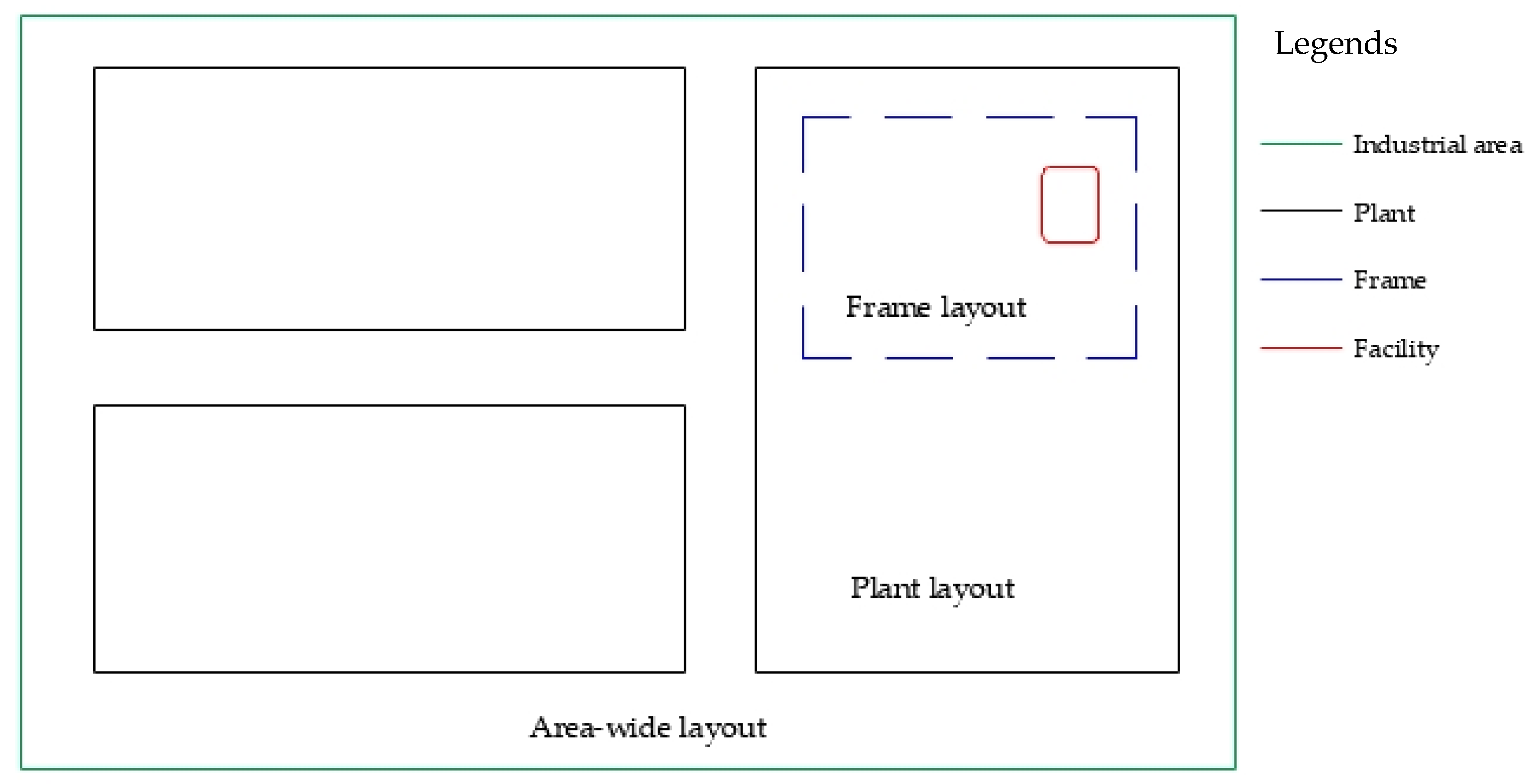
By studying previous work on layout design, it is found that two major problems have not been well studied. The first issue is the multiple frames problem. How to distribute facilities into different frames must be studied to keep the shortest connections between faculties. The second issue is the multiple floor problem. Although some efforts have been made regarding the multiple floor problem, when the multiple frames problem is raised, it is necessary to determine all the floor numbers of frames. Therefore, the main focus of this work can be described as the pursuit of a more practical plant layout with inner facilities arranged reasonably by considering the above-mentioned two issues. In this work, frames are added as a new sort of inner structure to fit the internal layout manner of an actual plant. After the addition of frames, the range of the various elements in FLPs can be intuitively comprehended in Figure 1. Then the frames are integrated into the plant layout. To divide facilities into several blocks, a quantitative mathematical model is proposed to form a few frames in the objective of minimizing the number of cross-frame connections. Each frame layout is optimized, and the floor number is determined in the objective of minimizing the total annual cost. A hybrid algorithm combing GA and surplus rectangle fill algorithm (SRFA) is used to do optimization in each frame to minimize total annual cost (TAC). Designer decisions are added to determine the relative frame locations and material handling points, so as to adjacently arrange frames with more material exchange. Then the internal layout of each frame is optimized again under the restriction of cross-frame connections, so as to reach the coupling optimization of frame layout and plant layout.
2. Mathematical Model and Algorithm
2.1. Problem Statement
FLPs generally possess great difficulty and long calculation time due to the large number of variables and constraints. For the sake of modeling, it is necessary to set a couple of assumptions and considerations to simplify the mathematical model.
- Plants, frames, and facilities are all regular rectangles and should be placed orthogonally;
- There are two levels of layouts involved in this work, which are frame layout and plant layout, increasing successively;
- Safety distances are considered both between facilities and between frames, according to the regulations;
- High facilities such as towers and reactors are placed apart from the frames in the plant layout;
- Facilities are arranged in a two-dimensional plane;
- Cylindrical facilities are regarded as rectangles during the optimization process;
- If necessary, multi-floor structure can be taken into consideration in the frame when there are plenty of facilities;
- If multiple floors are applied, attention to vertical transportations and floor requirement for special facilities should be paid. For instance, pumps should be placed on the first floor so as to avoid cavitation.
With the simplifications above, it is easier to set a model for the plant layout problem. Besides, some basic data is also required, such as facility number, sizes, and flow information. The obtained results after the modeling and optimization often consist of multiple aspects to form a complete plant layout, which are:
- Coordinates of each facility in the frame area;
- Relative locations of frames and high facilities;
- Various costs of each frame;
- Internal layout diagrams of frames and the whole plant.
2.2. Constraints
Frame layout dealing with multiple facilities usually considers more constraints than the plant layout, since facilities possess various shapes and functions. A few constraints are set to reach a reasonable and effective frame layout.
Facility orientation constraints are established to present the visual length and width of a facility in the frame region. When the term “length” is defined as the size parallel to x-axis and “width” is the size in y direction, there is a certain relationship between the visual and actual size of a facility. A binary variable d is defined to illustrate this relationship. It is stipulated that when di = 1, the facility is placed vertically, then the actual length is the visual width of the facility. On the contrary, when di = 0, it is arranged horizontally. Then the relationship between the visual and actual size of the facility can be described as follows:
where, li and wi are the visual length and width of facility i within a certain frame region; loi and woi are the actual length and width of the facility.
Non-overlapping constraints are used to prevent common area between facilities. These constraints concern the facility sizes and area and stipulate that no cross region of different facilities is allowed. Facility i and j are forced to meet one of the following four inequality constraints to avoid overlapping area:
where, xi and yi are the center coordinates of facility i, and xj and yj are the same for facility j; l and w are the visual length and width mentioned before. Inequalities (3)–(6) represent, respectively, that facility i is on the right, left, top, and bottom side of facility j.
Boundary constraints demand that the area of any facility cannot go beyond the frame area. Four constraints must be satisfied at the same time to limit the location of a facility:
where, L and W are the length and width of the frame.
Pump constraints are set to draw a rectangular area for pumps for the convenience of pump centralized management. Pumps are arranged neatly in each frame as a whole, in the manner of several rows and columns. To avoid irregular shapes in the model, pump area is stipulated as the smallest rectangle which contains all the pumps, even if it is not exactly filled by the pumps. Pump area is regarded as an ordinary facility to be optimized together with other facilities. When the relative locations of pumps within the pump area are obtained, their actual coordinates in the frame can be described as follows:
where, xpi and ypi are the center coordinates of pump i in the frame; xpa and ypa are the lower left coordinates of pump area; xpri and ypri are the center coordinates of pump i within the pump area.
Floor constraints for special facilities are necessary when there are multiple floors in the frame. It is common sense to place pumps on the first floor to avoid cavitation, and allocate air coolers to the top floor to ensure their cooling effect. These considerations are set as constraints in this model. Besides, parallel heat exchangers with similar function are also constrained to be placed as a whole.
2.3. Objective Function
Costs are usually served as the measure of layout performance [40,41]. In this work, total annual cost (TAC) is set as the objective function in each frame, including land cost (LC), floor cost (FC), pipeline construction cost (PCC) and material handling cost (MHC):
LC and FC are closely related to the frame area:
where, ULC and UFC are the unit land and floor cost (¥/m2); S is the frame area; Af is the annualized factor; I is the interest rate.
PCC is associated with the pipeline investment, which is calculated as follows:
where, UPC is the unit pipeline cost ($/m), which is obtained by the method proposed by Stijepovic and Linke [42]; MD is the Manhattan distance (m) between connected facilities.
where, A1–A4 are fixed parameters, which are respectively 0.82 $/kg, 185 $/m0.48, 6.8 $/m, and 295 $/m; wtpipe is the unit quality of pipelines (kg/m); Dout is the outer diameter of pipelines (m). They are determined by Equations (21)–(23) [42]:
where, Dinner is the inner diameter of pipelines (m); Q is the mass flow rate of the medium in the pipelines (kg/sec); ρ is the density (kg/m3), and u is the flow rate (m/s).
MHC is the cost of material handling, which is calculated by the cost of pump work in each year:
where, CE is the cost of unit energy ($/kW·h); H is the annual operating hours in each year (h/a); P is the pump work consumed by transporting materials (W), which can be calculated as follows:
where, hf is the energy consumed in material handling process, which is used to overcome the resistance and gravity (J/kg); η is the efficiency of pumps; λ is the friction coefficient; g is the gravity constant; z is the length of vertical material transportations (m). α is a binary variable which stipulates that if there is a connection that transports materials vertically from the bottom to the top, then α = 1; if not, α = 0.
2.4. Optimization Algorithm
Due to the large number of variables and constraints, there is great difficulty in solving FLPs. Therefore, algorithms are often applied to provide help for optimization. Since the algorithm is not taken as the focus of this work and few significant changes have been made to the basic settings of the algorithms mentioned, only a brief introduction is made for the two algorithms used and their combination approach.
Among the widely-used metaheuristics, GA has obvious advantages in dealing with layout problems and possesses strong global search ability [43,44]. There are plenty of individuals in GA, which can be matched with facilities in one-to-one correspondence. Genes on chromosomes can determine the performance of individuals. Similarly, multiple variables are set to decide the number, orientation, and placement order of facilities, the bottom length of the frame, and the facility number in each floor (if there is a multi-floor structure). Variables are arbitrarily valued within the pre-determined range to realize the randomness of the optimization. The fitness value is set as TAC, which means the performance of the frame layout is measured by costs. Through GA, desired solutions can be obtained, including facility arranging sequence and orientation, frame bottom length, and various costs.
However, although GA is proved to be a suitable algorithm due to its features, there are still disadvantages that impede the acquirement of the final precise layout. GA is hard to consider facility sizes and areas, and thus difficult to generate tight layouts. The targets of layout studies are always plenty of rectangles with different shapes and sizes. When considering unequal-area facilities and their safety distance, GA seems not to be competent enough to arrange all the facilities in a tight and efficient manner. Therefore, an additional algorithm is required to deal with these issues. Surplus rectangle fill algorithm (SRFA) [45,46] is a kind of algorithm with the ability to divide a rectangular plate into several smaller parts, the idea of which just coincides with the idea of arranging rectangular facilities in a rectangular area. SRFA establishes a residual rectangle data set to collect the available free space for the arrangement of target rectangles. It is applied to arrange facilities and obtain the final layout with facility coordinates in each floor.
Although it is suitable for arranging unequal-area rectangular facilities in a given region, SRFA cannot solve layout problems by itself because it is not eligible to minimize TAC through the iteration, and it requires some initial necessary conditions to reach a proper facility arrangement, such as facility placement order and orientation, and this information can be provided by GA. Therefore, it is combined with GA to form a hybrid algorithm to reach the optimization of the frame layout. The combination of the two algorithms can be simply described as follows. With the given information such as facility number and sizes, and the data generated by GA such as the facility placement orientation, order, and the frame bottom length, SRFA designs the internal precise layout by its residual rectangle data set, and acquires facility coordinates. These coordinates are then returned to GA as the input parameters to minimize TAC with flow information. After the iteration, the layout with the smallest fitness value is selected as the output result when the termination condition is satisfied. These two algorithms work together in this manner to realize the randomness of the hybrid algorithm and arrange facilities practically. As a result, reasonable layout results can be obtained. For a better understanding, Figure 2 shows the workflow of the hybrid algorithm intuitively. It should be noted that the algorithm is carried out in MATLAB 2018a, relative operators in GA are default in the toolbox.
3. Optimization Approach
In this work, frames are integrated into the model as a special structure in plant layout. Therefore, there are two levels of layouts in the design of a plant, which are frame layout for facilities and plant layout for frames. To divide facilities into several frames, a quantitative approach is required instead of a qualitative one. Frames are optimized for the first time to obtain initial sizes and layouts, and then arranged together with the high facilities according to the designer decisions. However, layout optimization of frames in the previous step only considers the internal material connections. Besides, within the frame area, positions of facilities with cross-frame connections are also affected by the relative locations of frames. The above factors may lead to suboptimal results of the first plant layout optimization. Therefore, in order to reach a coupling optimization between frame layout and plant layout, it is necessary to do the optimization in each frame for the second time in the addition of cross-frame connections, to obtain a final coupling layout of the plant. The above steps can be described in detail as follows.
- Facilities are classified according to their features. Attention to the floors of special facilities such as pumps and air coolers should be paid if there is a multi-floor structure in the frame. Parallel heat exchangers are required to be arranged as a whole. Pumps ought to be placed neatly in the pump area. High facilities like reactors and towers are put aside and not allocated into frames;
- Facilities except high ones are divided into several frames. The number of frames is determined according to the actual situation. The principle of the separation is to figure out the cutting positions with the least number of cross-frame connections being cut within a reasonable range. This approach will be described in detail in the later statements;
- According to the flow information, all the connections are then divided into two categories, which are internal connections within the frame and cross-frame connections;
- Each frame is optimized with the constraints and the objective function, using the hybrid algorithm. In this step, only internal connections are considered. After the optimization, initial sizes and layouts of frames can be obtained;
- Designer decisions are applied to the arrangement of frames and high facilities. Frames (or high facilities) with frequent material exchange are manually allocated adjacently as far as possible, to reduce the costs of cross-frame connections;
- Initial plant layout with initial frames is obtained;
- Due to the effect of frame positions on the locations of facilities possessing material exchange outside the frame, each frame is re-optimized by the addition of cross-frame connections, and the modified sizes of frames are acquired;
- The whole plant layout is updated with the modified frames. Comparisons are made to prove the reasonability and effectiveness of the modification.
As mentioned above, a quantitative method is proposed to assign facilities. One thing that should be noted is that designer decisions are added into the model in the step of arranging frames and high facilities, which prompts the plant layout more in line with the layout habits of designers. These frames and high facilities can be arranged by computational optimization theoretically, as the way of arranging facilities within the frame area in the previous step. However, the calculation results may lead to some situations that do not confirm to the actual plant layout. For instance, two high facilities (like towers) that are often located adjacently in an actual industrial plant may be placed far from each other through the calculation process because one of them has more material connections to other frames, which is against common sense in an actual plant. Besides, as the frame number is small and the size difference may be large, the optimization layout result may not be very neat, or the land utilization rate is not ideal. Therefore, adding designer decisions is a preferable measure to avoid the above issues.
A quantitative method is required in the step of allocating facilities into several groups. When the facilities are divided into frames, all the connections can be defined as internal ones and cross-frame ones. Since cross-frame connections usually require longer transportation distance, the reduction of these connections is theoretically in favor of the final plant layout. To minimize the number of cross-frame connections, some work needs to be done. All the facilities that need to be separated are arranged in a single-floor area. The hybrid algorithm is adopted in the objective function to minimize the total pipeline length (TL) in the direction of y-axis:
where, n is the number of all the material connections; Ply is the pipeline length of each connection, in y direction.
Figure 3 is a schematic diagram for this step. After the single-floor layout is obtained, facilities (shown as black blocks) can be simplified as center points (in red), and all the connections are drawn in the form of right-angle lines (in blue). Assuming that all the facilities are required to be separated into two frames, then only one cutting point is needed. The cutting line (in green) is set to be perpendicular to y-axis, and moves from the bottom to the top in order to select a best point with the minimum of cut connections. In Figure 3 it can be easily figured out that position cp is a reasonable position of the cutting point with only two connections cut. Besides, the position of cp is about the half of the frame width, which can form two frames with proper sizes. The two cut connections are defined to be cross-frame connections. When there are many more facilities in an actual plant, more cutting points are required to obtain more frames.
4. Case Study and Analysis
To verify the effectiveness of the proposed approach, a catalytic cracking plant with 138 facilities and 247 material connections is designed in detail. The selected case is pretty representative and comprehensive for most industrial parks, which arranges rectangular facilities in a rectangular region. The problem size is pretty large, and the facilities are rectangles (or regarded as rectangles) in different shapes and sizes. Facilities possess various functions and specific placement constraints. Parallel placement and centralized arrangement are both involved. Therefore, if this case is verified to be solved successfully, other types of block layout can be dealt with in this proposed methodology with small modifications according to the situation.
In this case, there are seven high facilities, which are riser reactor (RR), settler-regenerator (SR), fractionating tower (FT), stripping tower (ST), absorption-desorption tower (ADT), stabilization tower (STA), and reabsorption tower (RT). Basic data of sizes and categories of facilities and flow information have been already acquired. The remaining 131 facilities ought to be divided into several frames and then optimized in the objective of minimizing the pipeline length in the direction of y-axis, which is presented in Equation (27). The bottom length is set to be around 20 m, and the result diagram of facility separation is shown in Figure 4. The calculation process lasts around 300 s.
The result shows that the length and width of the whole layout are 22.80 m and 141.80 m, respectively. To obtain a neater layout, heat exchangers and air coolers are arranged in the same direction. A group of parallel heat exchangers is regarded as a whole, so only one center point remains when the diagram is simplified. All the connections are drawn as right-angle lines. Then, a cutting line which is parallel to x-axis is added into the simplified diagram, and goes from 0 to 141.8 m of the width in y-direction to search for proper cutting points. The relationship between the position of cutting point and the number of the cut connections is presented in Figure 5.
Considering the total layout width and the proper widths of frames, it is reasonable to equally divide the layout into four frames, the width of each is around 35 m. It means there should be three cutting points, whose locations are about 35 m, 70 m, and 105 m in y-direction. An appropriate cutting point means the minimum of the cut connections within the proper width range. According to the result data and Figure 5, three points are selected to be cutting points and separate facilities into four frames, which are shown in Table 1.
Four frames are named as A to D from the top to the bottom. For instance, frame D contains the facilities between 0 and 34.4 m in width. It can be easily figured out that in frame B and C, facilities are arranged more closely. Frame A mainly contains parallel heat exchangers and air coolers, which can be regarded as a frame for the centralized arrangement of facilities with similar functions. However, it should be noted that current sizes of frames are only used to assign facilities, which cannot be the final sizes.
In total, 23 material connections are cut according to Table 1. However, six connections of them are proved to be counted repeatedly, since these six connections are between frame A and C. They are counted twice because they cross three frames (from frame A to C) and two cutting lines. Thus, there are actually only 17 cut connections, which proves to be a better result of the facility assignment. The selected 17 connections are defined to be cross-frame connections.
Referring to the arranging manner of an actual plant, high facilities like towers and reactors should be placed on the edge of the frames, rather than inside the frames. Therefore, there are additional cross-frame connections transporting materials between towers (or reactors) and frames. The number of these connections is usually large and cannot be optimized because the towers and reactors are outside the frames. These connections are also defined as cross-frame connections. Table 2 shows the facility number and relative cross-frame connections of each frame.
With the steps above, four frames are finally determined. However, this step is only used to separate facilities into frames according to the objective of minimizing the pipeline length. The internal layout cannot be an optimal one when it is measured in costs, so that the sizes and layout are then optimized for minimizing TAC. Only internal connections are considered because the material handling points of cross-frame connections are not determined until the relative locations of frames are fixed. Besides, in order to prove the ability of proposed approach to deal with multi-floor structure, frame C is selected to be a double-floor layout due to its larger number of facilities and more complex material exchange, and other frames remain to be single-floor. If there is a plant with many more facilities to be studied, multi-floor structure can also be applied into more frames. The optimized layouts are obtained, and the initial frame sizes are listed in Table 3. The calculation process in each frame lasts around 300 seconds as well.
Through the layout design of the economic based optimization, the sizes and internal layouts have been adjusted to a more proper manner for the convenience of the further arrangement of the plant layout. Frame A to D are required to be arranged together with five towers and two reactors together in the plant area. Designer decisions are adopted to reach a more practical layout. There are conventional considerations that require a joint arrangement of FT and ST. In addition, RR and SR must also be placed next to each other due to the large amount of material exchange. To reach a neat plant layout, towers are arranged in a row. According to the frequency of material exchange, relative locations of frames and high facilities are manually adjusted. Initial plant layout is presented in Figure 6.
The initial plant layout embodies most of the considerations of designers. For instance, frame C is placed in the middle so as to realize more convenient material transportations with high facilities and other frames, because it has the most cross-frame connections. As a result, a tight and reasonable plant layout is obtained, and the material handling points of frames can be determined to be the midpoint of the frame edge in the direction of material transportation.
However, the initial results of frames are not that perfect, because the cross-frame connections are not taken into account. The positions of facilities having connections outside their frame will be affected to some extent. Theoretically, the facility with links to other frames will be forced to move in the direction of the attached frame. To reach optimal internal frame layouts, modifications of initial frames are required. Cross-frame connections are considered and added into the objective function. The aim remains to minimize the total cost in each frame, and modified results are shown in Table 4.
It can be seen from Table 4 that the sizes and areas of frame A, B, and D possess quite small changes. The variation in the area of frame C is a little larger, but the length and width do not change too much. So, the shapes of the four frames basically remain the same, which means the choice of material handling points are reasonable and can be applied into the modified plant layout. The relative locations of frames and high facilities are kept unchanged, as shown in Figure 7.
There are plenty of changes in the frames after the modification. Costs and pipeline length are the two main aspects that should be especially considered. As for the pipeline length, Table 5 presents the length comparison of cross-frame pipelines. It can be seen that most frames possess quite large reductions in cross-frame pipeline length. However, the length of cross-flame connections increases in frame B; the reason is that such design can significantly reduce the pipeline length for the other frames. Due to the large reduction of pipeline length in other frames, the slight increase in frame B has little change in the overall trend of the whole plant. In total, there is a 582.7 m reduction in the cross-frame connections, which is a 28.5% drop. Through the modification, a significant reduction is obtained, which proves the ability to shorten pipelines of the proposed methodology.
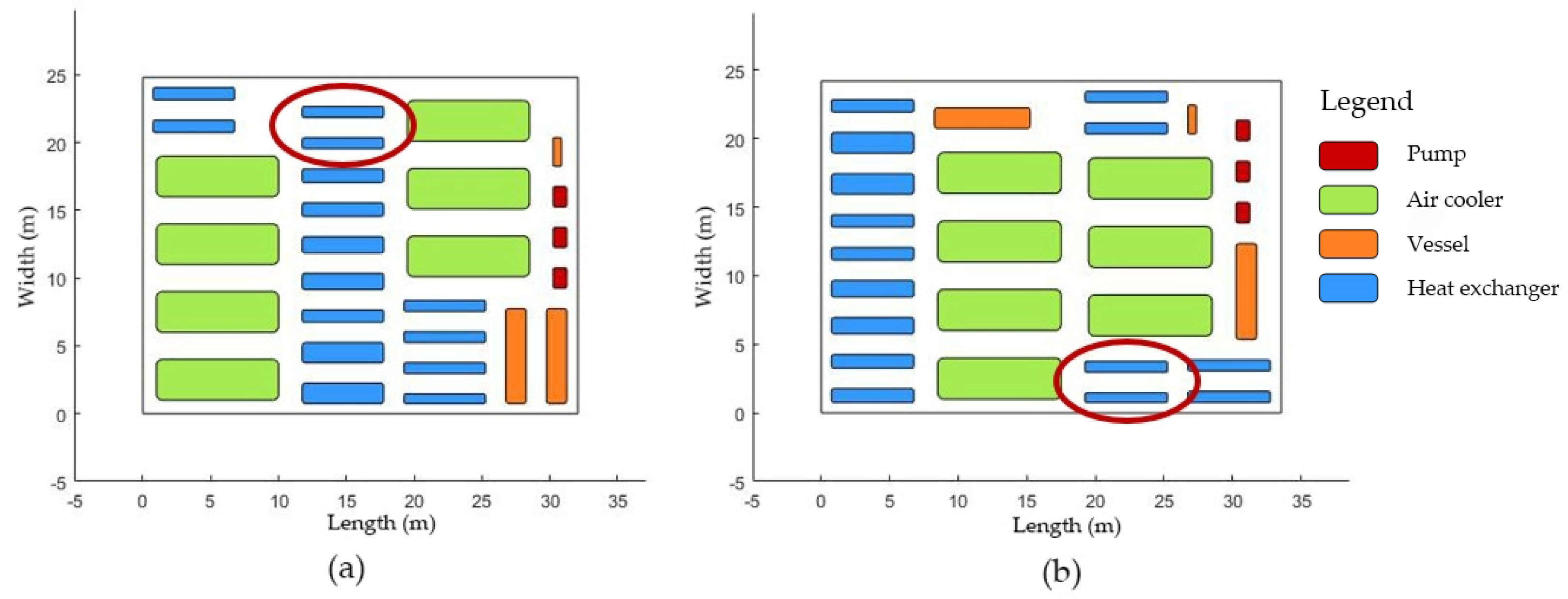
An example is taken to embody the pipeline length reduction of a specific facility. Figure 8a presents the initial layout of frame D, and Figure 8b is the modified frame layout for comparison. A set of parallel heat exchangers (circled in red) in frame D is chosen and studied. The two heat exchangers are arranged as a whole and possess two connections with RT. According to the plant layout in Figure 7, RT is arranged near the lower right corner of frame D, thus it is beneficial for facilities which are linked with RT to move in this direction, so as to shorten the pipelines. The studied heat exchangers are positioned at the top initially, and through the modification, they move to the lower place in the frame area. In the case that the frame shape basically remains the same, the position change of the studied facilities leads to 60.6 m reduction in the related pipeline length. Besides, other facilities also contribute to the decline in cross-frame pipeline length to varying extents, which results in a better plant layout with a significant reduction in the total length of cross-frame connections.
Pipeline length can be used to verify the performance of layouts but it is not comprehensive, so costs are selected to be the objective. Because the content of PCC and MHC in the objective function is adjusted before and after the modification, initial results are in the lack of the information of cross-frame connections, thus it makes no sense to directly contrast the calculation results of costs in the two scenarios. For comparison under uniform standards, PCC and MHC of cross-frame connections are calculated according to flow information and facility position, and are added into the costs of the initial results of each frame. Then the comparison is made. Various costs of initial and modified frames are listed in Table 6 and Table 7. Figure 9 shows the corresponding bar chart of Table 6 and Table 7. Four frames are compared respectively.
Comparing Table 6 and Table 7, and Figure 9, it can be figured out that the variation in LC and FC is relatively small, because the sizes and shapes of frames do not change too much. However, there are significant reductions in PCC and MHC in each frame after the modification. Analysis is made in two scenarios. Frames A, C, and D are involved in the first scenario. In these three frames, there is large decline in the pipeline length according to Table 5, which certainly results in the decrease in the related costs (PCC and MHC). Frame B is set as the other scenario with its modified pipeline length longer than the initial one. Even though the length is not reduced, the sum of PCC and MHC in frame B is still decreased. This is because there is difference in pipeline costs between cross-frame connections. Some connections are more expensive because they transfer more volume of fluid or their medium temperature is higher. Their costs are increased due to more pump work or better pipe materials. Relatively, other connections are cheaper. Therefore, a balance of facility positions is made to minimize the total costs. Cross-frame connections of higher price are shortened preferentially, and then other cheaper connections are considered. As a result, even if the pipeline length is not shortened, there is still an obvious reduction in TAC, especially in MHC. Considering all the frames in the plant, initial total cost is 1,936,624.26 ¥/a and modified total cost is 1,468,265 ¥/a. A reduction of 468,359.26 ¥/a is obtained, which turns out to be around a 31.9% drop.
As a conclusion, obvious decline is reached in both total costs and pipeline length in the plant area. Initial frame layouts acquire the sizes and relative locations but are proved to be suboptimal results due to the missing of cross-frame connections. Therefore, frames are re-optimized in the addition of cross-frame connections on the basis of determined material handling points, so as to reach a coupling optimization of frame layout and plant layout. As a result, after the modification, 582.7 m of pipeline length and 468,359.26 ¥/a of total cost are decreased.
5. Conclusions
In this work, efforts are made to reach a detailed and practical plant layout through several steps. Compared with previous works reported in literature, the main contribution of this work is establishing an optimization framework to achieve automatic arrangement of facilities in several frames. In this optimization framework, a new idea called “cutting point” is proposed to aid the division of frames through the different functional area of plants. The “cutting point” can boost the optimization process while providing adequate physical insight for the division. In the case study, our new proposed method can achieve a 468,359.26 ¥/a reduction of TAC and 582.7 m reduction in pipe length, which proves the effectiveness of the proposed method. The reason why such significant reduction can be achieved is that this work accurately describes and optimizes the cross-frame connection, and such connection has not been studied before.
As mentioned in the introduction, layout problems are complex and contain various aspects. This work emphasizes the division and connection of frames in layout design, but it misses a number of practical issues, e.g., safety issues. The lack of such practical issues makes our final layout designs far from real life situations. Therefore, one of the future directions is to combine as many practical factors as possible. Besides, manual operation is still required in this work. For the convenience of the application in the industry in the future, it is necessary to realize the complete automation of solution and combine the numerical results with a certain drawing software to output the layout directly in the form of general drawing in the future work.
Author Contributions
The work of raising the idea of frames and the optimization approach, setting models, and calculating the case is done by S.X. Guidance is provided by Y.W. and X.F. All authors have read and agreed to the published version of the manuscript.
Funding
This research was funded by Science Foundation of China University of Petroleum, Beijing (No.2462018BJC004).
Conflicts of Interest
The authors declare no conflict of interest.
References
- Drira, A.; Pierreval, H.; Hajri-Gabouj, S. Facility layout problems: A survey. Annu. Rev. Control 2007, 31, 255–267. [Google Scholar] [CrossRef]
- Koopmans, T.C.; Beckmann, M. Assignment Problems and the Location of Economic Activities. Econometrica 1957, 25, 53–76. [Google Scholar] [CrossRef]
- Garcia-Hernandez, L.; Salas-Morera, L.; Garcia-Hernandez, J.A.; Salcedo-Sanz, S.; de Oliveira, J.V. Applying the coral reefs optimization algorithm for solving unequal area facility layout problems. Expert Syst. Appl. 2019, 138, 13. [Google Scholar] [CrossRef]
- Abotaleb, I.; Nassar, K.; Hosny, O. Layout optimization of construction site facilities with dynamic freeform geometric representations. Autom. Constr. 2016, 66, 15–28. [Google Scholar] [CrossRef]
- Azevedo, M.M.; Crispim, J.A.; de Sousa, J.P. A dynamic multi-objective approach for the reconfigurable multi-facility layout problem. J. Manuf. Syst. 2017, 42, 140–152. [Google Scholar] [CrossRef]
- Meller, R.D.; Narayanan, V.; Vance, P.H. Optimal facility layout design. Oper. Res. Lett. 1998, 23, 117–127. [Google Scholar] [CrossRef]
- Ahmadi, A.; Pishvaee, M.S.; Jokar, M.R.A. A survey on multi-floor facility layout problems. Comput. Ind. Eng. 2017, 107, 158–170. [Google Scholar] [CrossRef]
- Wang, R.Q.; Zhao, H.; Wu, Y.; Wang, Y.F.; Feng, X.; Liu, M.X. An industrial facility layout design method considering energy saving based on surplus rectangle fill algorithm. Energy 2018, 158, 1038–1051. [Google Scholar] [CrossRef]
- Kalita, Z.; Datta, D. Multi-Objective Optimization of the Multi-Floor Facility Layout Problem; IEEE: New York, NY, USA, 2017; pp. 64–68. [Google Scholar]
- Meller, R.D.; Bozer, Y.A. Alternative approaches to solve the multi-floor facility layout problem. J. Manuf. Syst. 1997, 16, 192–203. [Google Scholar] [CrossRef]
- Barbosa-Povoa, A.P.; Mateus, R.; Novais, A.Q. Optimal design and layout of industrial facilities: A simultaneous approach. Ind. Eng. Chem. Res. 2002, 41, 3601–3609. [Google Scholar] [CrossRef]
- McKendall, A.R.; Shang, J.; Kuppusamy, S. Simulated annealing heuristics for the dynamic facility layout problem. Comput. Oper. Res. 2006, 33, 2431–2444. [Google Scholar] [CrossRef] [Green Version]
- Mir, M.; Imam, M.H. A hybrid optimization approach for layout design of unequal-area facilities. Comput. Ind. Eng. 2001, 39, 49–63. [Google Scholar] [CrossRef]
- Deb, S.K.; Bhattacharyya, B.; Sorhkel, S.K. Facility layout and material handling system selection planning using hybrid methodology. Int. J. Ind. Eng. Theory Appl. Pr. 2003, 10, 289–297. [Google Scholar]
- Durmaz, E.D.; Sahin, R. NSGA-II and goal programming approach for the multi-objective single row facility layout problem. J. Fac. Eng. Arch. Gazi Univ. 2017, 32, 941–955. [Google Scholar] [CrossRef]
- Ebrahimi, A.; Kia, R.; Komijan, A.R. Solving a mathematical model integrating unequal-area facilities layout and part scheduling in a cellular manufacturing system by a genetic algorithm. SpringerPlus 2016, 5, 29. [Google Scholar] [CrossRef] [Green Version]
- Ahumada, C.B.; Quddus, N.; Mannan, M.S. A method for facility layout optimisation including stochastic risk assessment. Process Saf. Environ. Prot. 2018, 117, 616–628. [Google Scholar] [CrossRef]
- Wang, R.Q.; Wu, Y.; Wang, Y.F.; Feng, X.; Liu, M.X. An layout optimization method for industrial facilities based on domino hazard index. In Proceedings of the 9th International Conference on Foundations of Computer-Aided Process Design, Copper Mountain, CO, USA, 14–18 July 2019; Munoz, S.G., Laird, C.D., Realff, M.J., Eds.; Elsevier: Amsterdam, The Netherlands, 2019; Volume 47, pp. 89–94. [Google Scholar]
- Zha, S.; Guo, Y.; Huang, S.; Fang, W. Dynamic facility layout for workshop under uncertain product demands. J. Jilin Univ. Eng. Technol. Ed. 2017, 47, 1811–1821. [Google Scholar]
- Liu, J.F.; Zhang, H.Y.; He, K.; Jiang, S.Y. Multi-objective particle swarm optimization algorithm based on objective space division for the unequal-area facility layout problem. Expert Syst. Appl. 2018, 102, 179–192. [Google Scholar] [CrossRef]
- Guan, C.; Zhang, Z.; Li, Y.; Jia, L. Combining Multi-objective Differential Evolution Algorithm and Linear Programming for Multiple Row Facility Layout Problem. J. Mech. Eng. 2019, 55, 160–174. [Google Scholar]
- Kulturel-Konak, S. The zone-based dynamic facility layout problem. INFOR 2019, 57, 1–31. [Google Scholar] [CrossRef]
- Friedrich, C.; Klausnitzer, A.; Lasch, R. Integrated slicing tree approach for solving the facility layout problem with input and output locations based on contour distance. Eur. J. Oper. Res. 2018, 270, 837–851. [Google Scholar] [CrossRef]
- Klausnitzer, A.; Lasch, R. Optimal facility layout and material handling network design. Comput. Oper. Res. 2019, 103, 237–251. [Google Scholar] [CrossRef]
- Wu, Y.; Wang, R.Q.; Wang, Y.F.; Feng, X. An area-wide layout design method considering piecewise steam piping and energy loss. Chem. Eng. Res. Des. 2018, 138, 405–417. [Google Scholar] [CrossRef]
- Lee, K.Y.; Han, S.N.; Roh, M.I. An improved genetic algorithm for facility layout problems having inner structure walls and passages. Comput. Oper. Res. 2003, 30, 117–138. [Google Scholar] [CrossRef]
- Zhang, L.; Zhang, Y.J. Solving the Facility Layout Problem with Genetic Algorithm; IEEE: New York, NY, USA, 2019; pp. 164–168. [Google Scholar]
- Sahinkoc, M.; Bilge, U. Facility layout problem with QAP formulation under scenario-based uncertainty. INFOR 2018, 56, 406–427. [Google Scholar] [CrossRef]
- Toloo, M.; Tavana, M.; Santos-Arteaga, F.J. An integrated data envelopment analysis and mixed integer non-linear programming model for linearizing the common set of weights. Cent. Eur. J. Oper. Res. 2019, 27, 887–904. [Google Scholar] [CrossRef]
- Allahyari, M.Z.; Azab, A. Mathematical modeling and multi-start search simulated annealing for unequal-area facility layout problem. Expert Syst. Appl. 2018, 91, 46–62. [Google Scholar] [CrossRef]
- Pierreval, H.; Caux, C.; Paris, J.L.; Viguier, F. Evolutionary approaches to the design and organization of manufacturing systems. Comput. Improbed Genet. Eng. 2003, 44, 339–364. [Google Scholar] [CrossRef]
- Palubeckis, G. Single row facility layout using multi-start simulated annealing. Comput. Ind. Eng. 2017, 103, 1–16. [Google Scholar] [CrossRef]
- Kulturel-Konak, S. A Matheuristic Approach for Solving the Dynamic Facility Layout Problem. In International Conference on Computational Science; Koumoutsakos, P., Lees, M., Krzhizhanovskaya, V., Dongarra, J., Sloot, P., Eds.; Elsevier: Amsterdam, The Netherlands, 2017; Volume 108, pp. 1374–1383. [Google Scholar]
- Jeong, D.; Seo, Y. Golden section search and hybrid tabu search-simulated annealing for layout design of unequal-sized facilities with fixed input and output points. Int. J. Ind. Eng. Theory Appl. Pr. 2018, 25, 297–315. [Google Scholar]
- Vitayasak, S.; Pongcharoen, P.; Hicks, C. A tool for solving stochastic dynamic facility layout problems with stochastic demand using either a Genetic Algorithm or modified Backtracking Search Algorithm. Int. J. Prod. Econ. 2017, 190, 146–157. [Google Scholar] [CrossRef] [Green Version]
- Montreuil, B.; Ratliff, H.D. Optimizing the location of input/output stations within facilities layout. Eng. Costs Prod. Econ. 1988, 14, 177–187. [Google Scholar] [CrossRef]
- Xiao, Y.J.; Zheng, Y.; Zhang, L.M.; Kuo, Y.H. A combined zone-LP and simulated annealing algorithm for unequal-area facility layout problem. Adv. Prod. Eng. Manag. 2016, 11, 259–270. [Google Scholar] [CrossRef] [Green Version]
- Leno, I.J.; Sankar, S.S.; Ponnambalam, S.G. An elitist strategy genetic algorithm using simulated annealing algorithm as local search for facility layout design. Int. J. Adv. Manuf. Technol. 2016, 84, 787–799. [Google Scholar] [CrossRef]
- Meller, R.D.; Kirkizoglu, Z.; Chen, W.P. A new optimization model to support a bottom-up approach to facility design. Comput. Oper. Res. 2010, 37, 42–49. [Google Scholar] [CrossRef]
- McKendall, A.R.; Shang, J. Hybrid ant systems for the dynamic facility layout problem. Comput. Oper. Res. 2006, 33, 790–803. [Google Scholar] [CrossRef]
- Zha, S.S.; Guo, Y.; Huang, S.H.; Wu, Q.; Tang, P.Z. A hybrid optimization approach for unequal-sized dynamic facility layout problems under fuzzy random demands. Proc. Inst. Mech. Eng. Part B J. Eng. Manuf. 2019, 18. [Google Scholar] [CrossRef]
- Stijepovic, M.Z.; Linke, P. Optimal waste heat recovery and reuse in industrial zones. Energy 2011, 36, 4019–4031. [Google Scholar] [CrossRef]
- Gomez, A.; Fernandez, I.; De La Fuente, D.; Puente, J. Using genetic algorithms to resolve layout problems in facilities where there are aisles. Int. J. Prod. Econ. 2003, 84, 271–282. [Google Scholar] [CrossRef]
- Yu, R.; Wang, Y.; Peng, H. Improved genetic algorithm for workplace facility layout. J. Tsinghua Univ. Sci. Technol. 2003, 43, 1351–1354. [Google Scholar]
- Tao, W.; Wang, H.; Li, Z. Optimal Solution of Rectangular Part Layout Based on Rectangle-Filling Algorithm. China Mech. Eng. 2003, 14, 1104–1107. [Google Scholar]
- Zhao, H.; Wang, Y.; Feng, X. Optimization of area-wide layout in petrochemical plant with multiple sets of facilities. Petrochem. Technol. 2017, 46, 938–943. [Google Scholar]
Figure 1.
Various elements in layout problems.

Figure 2.
Flow diagram of the hybrid algorithm.

Figure 3.
Schematic diagram for choosing cutting points.

Figure 4.
Layout for facility separation of the studied catalytic cracking plant.

Figure 5.
Diagram for finding proper cutting points.

Figure 6.
Initial plant layout diagram.

Figure 7.
Modified plant layout diagram.

Figure 8.
Internal layout of (a) initial frame D and (b) modified frame D.

Figure 9.
Cost comparison of four frames.


Table 1.
Information of chosen cutting points.
| Number | Precise Position in Width (m) | Number of Cut Connections |
|---|---|---|
| 1 | 34.4 | 8 |
| 2 | 74.6 | 10 |
| 3 | 98.5 | 5 |
Table 2.
Information of each frame about the facility number and cross-frame connections.
| Frame | Number of Facilities Inside | Number of Connections between This Frame and Other Frames | Number of Connections between This Frame and High Facilities |
|---|---|---|---|
| A | 30 | 8 | 10 |
| B | 27 | 6 | 16 |
| C | 46 | 15 | 32 |
| D | 28 | 5 | 14 |
Table 3.
Initial sizes of frames.
| Frame | Length (m) | Width (m) | Area (m2) |
|---|---|---|---|
| A | 20 | 47.3 | 946 |
| B | 20.23 | 25 | 505.75 |
| C | 20.28 | 25.3 | 513.08 |
| D | 32.07 | 24.8 | 795.34 |
Table 4.
Modified sizes and area change rate of frames.
| Frame | Length (m) | Width (m) | Area (m2) | Rate of Area Change (%) |
|---|---|---|---|---|
| A | 23.66 | 42.4 | 1003.18 | 5.70 |
| B | 20.03 | 26.5 | 536.1 | 5.65 |
| C | 20 | 22.1 | 442 | 16.08 |
| D | 32.88 | 24.6 | 808.85 | 1.67 |
Table 5.
Comparison of cross-frame pipeline length.
| Pipeline Length of Cross-Frame Connections | Frame A | Frame B | Frame C | Frame D | Total |
|---|---|---|---|---|---|
| Initial layout (m) | 599.38 | 335.28 | 1349.16 | 343.16 | 2626.98 |
| Modified layout (m) | 358.58 | 344.18 | 1158.18 | 183.34 | 2044.28 |
| The reduction in modified layout (m) | 240.80 | −8.9 | 190.98 | 159.82 | 582.70 |
Table 6.
Costs of initial frames.
| Frame | LC (¥/a) | FC (¥/a) | PCC (¥/a) | MHC (¥/a) | TAC (¥/a) | Total (¥/a) |
|---|---|---|---|---|---|---|
| A | 94600 | 0 | 49,099.7 | 43,388.04 | 18,7087.74 | 1,936,624.26 |
| B | 50,576.47 | 0 | 29,123.97 | 162,662.27 | 24,2362.71 | |
| C | 51,297.53 | 30,778.51 | 84,501.54 | 1,226,642.43 | 1,393,220.01 | |
| D | 79,528.23 | 0 | 28,896.76 | 5528.81 | 113,953.8 |
Table 7.
Costs of modified frames.
| Frame | LC (¥/a) | FC (¥/a) | PCC (¥/a) | MHC (¥/a) | TAC (¥/a) | Total (¥/a) |
|---|---|---|---|---|---|---|
| A | 100,305.32 | 0 | 38,202.18 | 14,788.58 | 153,296.08 | 1,468,265 |
| B | 53,071.62 | 0 | 33,515.89 | 130,046.78 | 216,634.29 | |
| C | 44,208.7 | 26,525.22 | 62,270.57 | 854,591.02 | 987,595.51 | |
| D | 80,874.96 | 0 | 25,136.95 | 4727.21 | 110,739.12 |
© 2020 by the authors. Licensee MDPI, Basel, Switzerland. This article is an open access article distributed under the terms and conditions of the Creative Commons Attribution (CC BY) license (http://creativecommons.org/licenses/by/4.0/).
Share and Cite
MDPI and ACS Style
Xu, S.; Wang, Y.; Feng, X. Plant Layout Optimization for Chemical Industry Considering Inner Frame Structure Design. Sustainability 2020, 12, 2476. https://doi.org/10.3390/su12062476
AMA Style
Xu S, Wang Y, Feng X. Plant Layout Optimization for Chemical Industry Considering Inner Frame Structure Design. Sustainability. 2020; 12(6):2476. https://doi.org/10.3390/su12062476
Chicago/Turabian StyleXu, Siyu, Yufei Wang, and Xiao Feng. 2020. "Plant Layout Optimization for Chemical Industry Considering Inner Frame Structure Design" Sustainability 12, no. 6: 2476. https://doi.org/10.3390/su12062476
Note that from the first issue of 2016, this journal uses article numbers instead of page numbers. See further details here.