Abstract
The development of agricultural services was the most important change in China’s agricultural production in the past 20 years. Using nationally representative provincial-level panel data, this study shows that agricultural service has a positive impact on technical efficiency at a significance level of 0.06. Based on this study, if the share of agricultural service cost increases by 1%, technical efficiency will increase by 0.35%. In other words, this study provides an empirical explanation of the positive impact of agricultural service on productivity. Due to the heterogeneity of agricultural service, technical efficiency in Eastern China and major grain production regions is higher than that in other regions. Finally, this study confirms the convergence of technical change in China’s grain production.
1. Introduction
Agricultural service in China was unimportant until the early 2000s. As in other developing countries where there were millions of small households, China had a large pool of surplus labor in rural areas after the agricultural reform at the end of 1970s [,,,]. The continuous migration of these surplus rural laborers to cities significantly has changed China’s economic development during the past four decades [,,]. Correspondingly, demand for agricultural service was low in rural China. In this study, agricultural service is defined as a service for farmers during crop production, such as soil preparation, pest and disease control, and harvesting, etc. According to the statistics of the All China Data Compilation of the Costs and Returns of Main Agricultural Products, the real service cost in 1999 was less than 1.5 times higher than that in 1978 [].
In recent years, however, the expenditure on agricultural service has become the largest material cost in agricultural production. Even though it was believed that there were millions of surplus rural laborers waiting to migrate to cities, the continuous migration finally led to the substantial increase in wage rate [,,,]. The rising wage rate declared the emergence of the Lewis turning point, which is named after the economist W. Arthur Lewis and is a situation where surplus labor in rural areas is fully absorbed into the non-farm sector [,,,]. To offset the reduction of labor input in agricultural production, the development of agricultural service accelerated in the last two decades [,,]. According to national statistics, the service cost increased by more than three-fold during the period 2000–2017, making it the largest material cost in agricultural production [].
Given the importance of agricultural service, it is surprising to find that few studies have focused on the impact of agricultural service on agricultural production in China. There are lots of questions that need to be investigated. For example, did agricultural service lead to any change of crop productivity (i.e., yield)? If yes, what is the mechanism of this change? These questions are waiting for satisfactory answers.
The objective of this study is to answer these questions. Specially, this study has three objectives. First, this study will document the development of agricultural service in China. Second, this study will identify the impact of agricultural service on crop productivity. Finally, this study will discuss the impact of agricultural service on the dynamics of technical change (TC) and technical efficiency (TE) over time.
However, due to the concerns about data availability, this study restricts the analysis to three major grain crops: rice, wheat and corn. Focusing on these three grain crops should still be of interest because these three crops are the largest grain crops in China. According to national statistics, the total sown area of these three grain crops is 96.59 million hectare (ha), which is 82.52% of the total sown area of all grain crops, and 58.22% of the total sown area of all crops in China in 2018 [].
The rest of this paper is organized as follows. In the next section, this study will describe the development of agricultural service in China’s agricultural production. In the third section, the data source will be discussed. Then, this study will set up and estimate the production functions to identify the impact of agricultural service on crop productivity and TE. The final section concludes the paper.
2. Background of Agricultural Service in China
Agricultural service is ignorable in the 1980s and 1990s. During the agricultural reform at the end of the 1970s, nearly 100 million ha of collectively-owned arable land was allocated (mostly according to family size) to more than 200 million small households [,,]. After the reform, China’s agriculture had the characteristics of extremely small farm sizes (usually less than one ha) and land fragmentation (i.e., each household has several pieces of land), which had important implications for China’s agriculture production mode []. More importantly, as the largest populous country, China had approximately 800 million people living in rural areas in the 1980s []. Hence, labor input in agricultural production was over supplied, while the demand for agricultural service was low.
However, a rapid increase in wage rates significantly changed the development of agricultural service since the early 2000s. Although it was thought that there were millions of surplus laborers in rural China, the Lewis turning point appeared with repeated reports of a shortage of laborers and a rapid increase in wage rates in the early 2000s [,,,]. Wages rising attracted even more rural laborers to migrate to cities. According to national statistics, the rural–urban migration of 2018 was 288.4 million, which was more than half of the rural population []. It is uneconomic for migrants to return to their hometowns, which are usually several hundred miles away, and perform agricultural activities (for example, irrigation or pesticide spraying). Consequently, agricultural service has become common in recent years.
The development of agricultural services accelerated for two more additional reasons. First, the Chinese government provided substantial subsidies (e.g., for purchasing large and medium-sized agricultural machinery) since 2004 to encourage the development of mechanization []). Second, the development of the professional agricultural service organizations further contributed to the development of agricultural service in practice [,]. These professional agricultural service organizations have highly efficient agricultural machines which successfully satisfy the farm-level labor constraints, in particular during the agricultural peak seasons.
The development of agricultural service significantly changed the production mode and has important implications. First of all, agricultural service significantly changed the cost structure in production. With the development of agricultural service, the family labor input reduced while the agricultural service cost increased. As shown in Figure 1, the total expenditure on agricultural service increased continuously since the early 2000s, and surpassed the fertilizer cost in 2010. Since then, the agricultural service cost became the largest material cost in production.
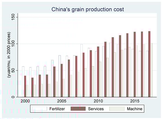
Figure 1.
Fertilizer cost, the agricultural service cost and the machine cost in China’s grain production.
Second, the development of agricultural service might have contributed to the increase in productivity. Since machines are widely used by agricultural service providers, mechanization has been used as an index of agricultural service in previous studies. This study also uses mechanization (i.e., machine cost) as an alternative variable to measure agricultural service. Previous studies showed that mechanization might be positively related to high productivity []. Agricultural services, especially those provided by skilled workers who could operate efficiently in timing and method, could contribute to an increase in crop yields []. For example, a large-size harvesting machine can harvest approximately one hundred hectares of wheat in two weeks, which helps to avoid the potential yield loss caused by heavy rain, which is very common in China’s major wheat production regions during the harvesting season. Similarly, agricultural service provided by a skilled worker who knows the most efficient way to spray pesticide at the right time can help increase crop yields.
3. Methods
In this section, the author will first discuss the data used in this study. Then, the author will estimate a fixed effect model in which agricultural service is treated as the same as other agricultural inputs (e.g., fertilizer and labor). As there is an interaction term between agricultural service and time, the estimation results of the model will show whether the impact of agricultural service on crop yield increases over time. If a rising impact is confirmed, the author will then estimate a stochastic frontier production function to explain the mechanism of the rising impact. The stochastic frontier production function provides estimations for the parameters of a linear model with a disturbance and a stochastic technical efficiency which is assumed to be a strictly nonnegative and symmetric distribution, respectively [,]. The stochastic frontier production function has been widely used to estimate technical efficiency, which is measured by the ratio of observed output to the maximum feasible output. Finally, the characteristics of calculated values of TE and TC will be discussed.
3.1. Data Source
The data used in this study had two main sources: the China Statistical Yearbook (Zhongguo Tongji Nianjian) and the All China Data Compilation of the Costs and Returns of Main Agricultural Products (Quanguo Nongchanpin Chengben Shouyi Ziliao Huibian). Specifically, major input (such as labor, fertilizer, service, machine, and others) and output (i.e., yield) data were from the All China Data Compilation of the Costs and Returns of Main Agricultural Products []. The Consumer Price Index (CPI) data are from the China Statistical Yearbook []. To avoid the impact of price inflation over time, all the cost data were adjusted by CPI (with CPI = 100 in the year 2000). The basic characteristics of the major variables used in this study are summarized in Table 1.

Table 1.
Basis characteristics of the major variables used in this study.
Before the discussion of the data in detail, the author would like to talk about the choice of time period. First, the state’s monopoly on the purchase and marketing of agricultural products was not completely removed until the middle of the 1990s in China []. Second, a shortage of labor and a continually increasing wage rate did not appear until the early 2000s [,,]. Consistently, the service cost (and machine cost) increased significantly since the early 2000s (Figure 1). As the objective of this study is to understand the impact of agricultural service, the time period of 2000–2017 was selected for empirical estimation.
To avoid the possible estimation bias, the author deleted 10 observations which had less than five observations for one crop in one province. These 10 observations were the Japanic rice of Beijing in 2000, the middle rice of Jiangxi and Zhejiang in 2004, the wheat of Zhejiang during the period 2000–2002, the corn of Hunan in 2001, the wheat of Liaoning in 2000, and the wheat of Tibet during the period 2002–2003. Removing these 10 observations led to the 1470 total observations used for this study.
3.2. Dynamic of the Impact of Service over Time?
As the first step of empirical analysis, the author set up and estimated a widely-used traditional fixed effect production function as follows:
In Equation (1), Yield is measured by kg per unit of land (i.e., mu). Service is the total expenditure on agricultural service, while Fertilizer is the total expenditure on chemical fertilizer. The reason that fertilizer input is separated from other inputs is that the fertilizer cost was the largest material cost until its rank was replaced by the service cost in recent years. The other cost, Other, was calculated using the following equation: other cost = total production cost − labor cost − fertilizer cost − agricultural service cost.
Labor was used to capture the impact of labor input on grain yield. Due to the rapid increase in wage rates in the past two decades, the dynamics of labor cost show a clearly increasing trend over time. However, rural–urban migration led to the continuing reduction of labor input in agricultural production in practice. Hence, the increasing labor cost data series could not represent the impact of labor input on grain production. For this reason, the number of labor days during the agricultural production was used in Equation (1).
Finally, three vectors of dummies, Province, Crop and Year, were used to capture the impact of the heterogeneities caused by geographic, crop and time trend. In other words, this study considers the yield difference caused by different crops, the impact of geographic differences (i.e., province dummies), and the impact of climate change (i.e., year dummies). Adding these three groups of dummy variables also makes the Equation (1) a three-way fixed effect model. Equation (1) was estimated using Stata (a commonly used statistical software) and build-in regress command which is the most used method in applied econometric analysis.
The estimation results of Equation (1) are shown in Table 2. As shown in the first column of Table 2, most of the estimated coefficients have the expected signs. For example, the estimated coefficients of fertilizer, agricultural service, and other costs are all positive and statistically significant, indicating that they have a positive impact on grain yield. On the other hand, the impact of labor is insignificant which is also common in similar previous studies [].
Table 2.
A three-way fixed effect of (natural log of) grain yield.
However, the estimation results do not show whether the impact of agricultural service on grain yield changes over time. In Equation (1), the impact of service was assumed to be constant over time. To answer whether the impact of agricultural service on grain yield increases or decreases over time, an interaction term of service and time (i.e., Service * Year) was added into Equation (1). The estimation results, as shown in the second column of Table 2, are very similar to that in column 1, indicating the estimated results were robust. More importantly, the estimated coefficient of the interaction term is positive and statistically significant (row 5). In other words, the estimation results show that the positive impact of agricultural service on grain yield increased over time.
To check the robustness of the estimation results, the author reran the model under two scenarios. First, another interaction term, fertilizer and year (i.e., Fertilizer * Year), was added in Equation (1). The estimation results, as shown in the third column of Table 2, are as expected. The estimated coefficient of the new added interaction term is statistically insignificant, indicating that the impact of fertilizer on yield is constant over time. More importantly, adding the new interaction term did not lead to a significant change in the estimated coefficient of the interaction term of agricultural service and time. That is, the estimated coefficient of the interaction term of agricultural service and time trend is still positive and statistically significant.
Second, the author reran the models by replacing the agricultural service cost by machine cost. As discussed above, machine cost is the most important component of the agricultural service cost. In other words, the machine cost is a good representative of agricultural service cost. To check the robustness of the estimation results, the total service cost was replaced by the machine cost in the estimation and Equation (1) was re-estimated. The estimation results are shown in the 4th–6th columns of Table 2. The estimation results shown in the last three columns are very similar to those of the first three columns. In other words, the positive impact of agricultural service on crop yield and its increasing trends over time are robust.
3.3. Why Did the Impact of Service Increase over Time?
The estimation results of Equation (1), as shown in Table 2, confirmed that the impact of agricultural service on grain yield increased over time. However, the traditional production model (i.e., Equation (1)) could not provide an explanation behind the increasing positive impact. This is why the impact of agricultural service on grain yield increased over time remains unclear. In order words, Table 2 does not show whether the crop yield increase was realized by the introduction of new technology or the improvement of technical efficiency.
Even though agricultural service might have no direct impact on technical change, it might have a positive impact on technical efficiency. As discussed in the second section, skilled workers who provide agricultural service might be more efficient in operating agricultural practices, such as timing and operating method. As a result, agricultural service might have a positive impact on technical efficiency. In other words, the increase in crop yields, as shown in Table 2, might come from the increase in technical efficiency resulting from agricultural service.
To test whether agricultural service has a positive impact on technical efficiency, the author then estimated a stochastic frontier production model as follows:
In Equation (2), all the other variables were explained except for u. u is a non-negative random variable representing technical inefficiency, which is assumed to follow an exponential distribution. The inefficiency equation is assumed as follows:
Here, the Share_service is the share of the agricultural service cost in the total production cost. If the estimated coefficient of this variable is negative and statistically significant, technical inefficiency will decrease (i.e., technical efficiency will increase) as the share of agricultural service increases. The Year variable is added to consider the impact of the time trend on technical efficiency. Equations (2) and (3) were estimated using the build-in frontier command in Stata.
The estimation results of Equations (2) and (3) are shown in Table 3. As expected, all the inputs (i.e., labor, fertilizer, service or machine, other input) have positive impacts on grain yield and are statistically significant. For example, the estimated coefficient of fertilizer is positive and statistically significant, indicating that fertilizer has a positive impact on grain yield potential. Similarly, the positive estimated coefficient of agricultural service indicates that the production frontier moves up as more agricultural service is used.
Table 3.
Estimation results of the frontier production function and the determinants of technical efficiency.
More importantly, the estimation results show that agricultural service has a positive impact on technical efficiency. As shown in the fifth row of Table 3, the estimated coefficient of the share of agricultural service is −2.57 with a p-value of 0.06. As discussed above, the negative estimated coefficient indicates an increase in share of agricultural service cost will lead to a decrease in technical inefficiency. In other words, as the share of agricultural service cost increases, technical efficiency will increase. Based on the estimation results, if the share of agricultural service cost increases by 1%, technical efficiency will increase by 0.35% (2.57 × 1% × 0.12/0.88 = 0.35%). Replacing the agricultural service cost with the machine cost (the other cost was recalculated correspondingly, and the share of the agricultural service cost was replaced by the share of the machine cost in the technical inefficiency function) yields similar results (sixth row of Table 3).
3.4. TE over Time and Province
In this sub-section, the author will first calculate the values of TE. After the estimation of Equations (2) and (3), the values of TE can be predicted using the build-in predict command in Stata. Then, the author will show and discuss the basic characteristics of the calculated values of TE. By doing so, the author would like to summarize some characteristics of crops and/or provinces of TE over time. These findings are summarized as follows.
The first finding is that the values of TE increased over time (Figure 2). To make the dynamic clearer, Figure 2 smoothed the changes of TE over time. The smoothed curve of TE, as shown in Panel A, shows a very clear increasing trend over time. In other words, the calculated values of TE increase over time. To check the robustness of this finding (e.g., whether the increasing trend of TE is caused by outliers, etc.), the author then showed the dynamics of TE for wheat, corn and rice, respectively. Panels B–D of Figure 2 show that the increasing trend of TE over time is obvious for all crops. That is, the improvement of TE over time is universal across crops.
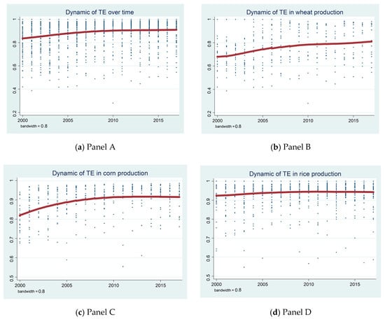
Figure 2.
Dynamics of technical efficiency (TE) over time.
The second finding is that the values of TE in Eastern China are higher than those in Western China. As shown in Figure 3, the top 10 provinces with the highest values of TE are: Zhejiang, Qinghai, Jiangxi, Hunan, Anhui, Shandong, Fujian, Guangdong, Jilin, Liaoning provinces (Panel A). Five of these 10 provinces are located in Eastern China, while the other four provinces that are located in Central China (i.e., Jiangxi, Hunan, Anhui and Jilin provinces) are major grain-producing provinces. The high efficiency of the Qinghai province seems to be related with its low technical change, which will be discussed in the following. On the other hand, six of the 10 provinces and autonomous regions with the lowest values of TE are from Western China: Yunnan, Gansu, Guizhou, Xinjiang, Ningxia and Sichuan, while the other two municipalities with low values of TE are Beijing and Shanghai, which are China’s commercial capitals where the percentages of agricultural GDP are less than 0.5% in the total GDP [].
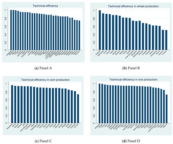
Figure 3.
TE across provinces.
This finding holds if TE across crops is checked (Panels B–D of Figure 3). For example, four of the bottom five provinces with the lowest values of TE in wheat production are from Western China (the other province is located in Central China), while four of the top five provinces with the highest values of TE are China’s major grain-producing provinces (Panel B). Similarly, all three provinces with the lowest values of TE in corn production are from Western China, while all the other provinces have similar values of calculated TE (Panel C).
This interesting finding is consistent with the positive impact of agricultural service on TE as shown in Table 3. Due to the regional disparities in China’s economic growth, the average wage rate in Western China is lower than that in Eastern China. A high wage rate leads to increasing demand for agricultural service in Eastern China. Figure 4 shows that the average agricultural service cost (and machine cost) is higher in Eastern China than that in Western China. As shown in Table 3, the increase in agricultural service has contributed to the increase in TE in Eastern China. That is, the high values of TE, at least partly, can be explained by the high values of agricultural service cost in Eastern China.
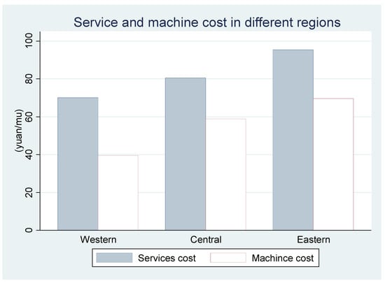
Figure 4.
Service cost and machine cost in different regions.
However, the positive impact of agricultural service itself could not assure the values of TE in Eastern China, which are higher than those in Western China because TE is also affected by other factors. For example, another important factor affecting TE is the introduction of new technology [,]. Since it takes time for adopters to understand the new technology and operate it in practice, the introduction of new technology has a negative impact on TE [,]. On the other hand, TE increases over time. Hence, the higher values of TE in Eastern China seem to hint that technology adoption in Eastern China might be slower than that in Western China. To test whether it is right, the author will check the technical change in different regions in the following.
3.5. Convergence of Technology Expansion
According to Equation (2), the total factor productivity (TFP) is calculated as following Equation (4):
As discussed above, all the values in Equation (2) are in their natural log forms. After obtaining the natural log of TFP, the author then calculated the absolute value of TFP and the annual growth rate of TFP.
Figure 5 shows that the TFP has a clear increasing trend over time (Panel A). To make the dynamics of TFP over time clearer, the author smoothed the changes in Figure 5. The smoothed curves show a very clear increasing trend over time. This finding holds not only for all grain crops, but also for wheat, corn and rice crops, respectively. That is, Figure 5 shows that the contribution of non-input factors (i.e., technical change and/or technical efficiency) on grain yield increases over time. The dynamics of TFP, as shown in Figure 5, are not only consistent with the increasing grain yield over time, but also provide evidence that the estimation results of stochastic frontier production models are reliable.
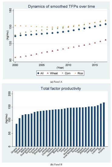
Figure 5.
Dynamics of total factor productivities (TFPs) over time and provinces.
The author further tested the hypotheses of the convergence of TFP. The idea of convergence (also sometimes known as the catch-up effect) is the hypothesis that provinces with lower values of TFP can replicate the production methods and technologies, and will tend to grow at faster rates than those with high values of TFP. As a result, the values of TFP of all provinces will eventually be similar, which is also considered as converging in terms of TFP. As shown in Panel A of Figure 6, the percentage increase in TFP has a clear negative relationship with TFP at a previous time. The β convergence is then confirmed in Table 4 (the first two columns) when the impact of other variables is excluded. Further study shows that there is no evidence of an overall σ convergence across all provinces. The results of the convergence test of this study are consistent with previous studies [,].
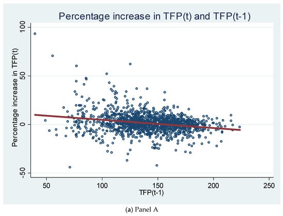
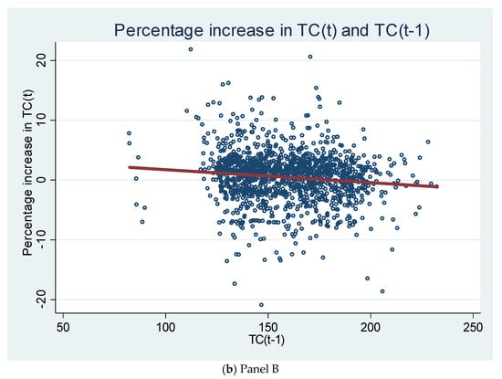
Figure 6.
Convergence of TFP and technical change (TC) over time.
Table 4.
Convergence of TFP and TE across provinces over time.
After calculating and discussing the TFP, the author then calculated the technical change on the grain yield using the following Equation (5):
The average impact of technical change on grain yield is shown in Figure 7. Panel A of Figure 7 shows that values of TC in Western China seem to be higher than that in Eastern China. For example, four of the top five provinces and autonomous regions with the highest values of TC are from Western China (i.e., Xinjiang, Gansu, Yunnan and Ningxia) and the remaining one province (i.e., Shanxi) is located in Central China. On the other hand, five of the bottom 10 provinces and municipalities with the lowest values of TC are from Eastern China: Guangdong, Hainan, Fujian, Zhejiang and Beijing. To make the comparison clearer, the author then calculated the average values of TC of the Eastern, Central and Western regions. Panel B of Figure 7 shows that the average value of TC of Western China is higher than that of Central China, while Eastern China has the lowest average value of TC. Further study shows that this finding holds for all the studied year.
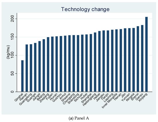
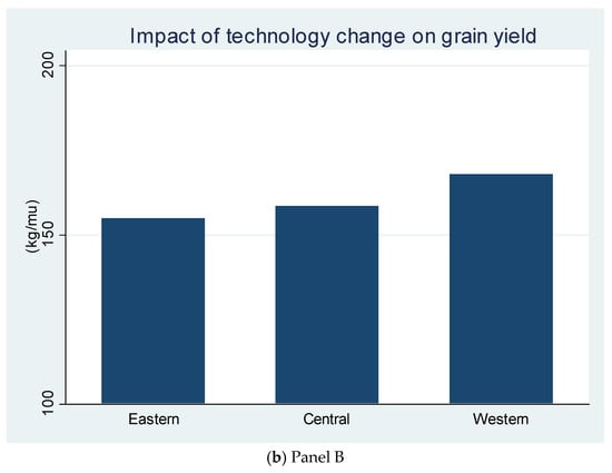
Figure 7.
TC across provinces and regions.
This finding is consistent with the dynamics of TE as shown in Figure 3. As discussed above, if all the other things hold constant, the realization of a high value of TE in one province requires that technical change in this province is slower than that of other provinces. Figure 3 and Figure 7 show that the technology growth rate in Western China is higher, while Eastern China enjoys the benefit of a higher TE.
It should be pointed out that this result is not surprising for at least two reasons. First, due to the importance of agriculture, the Chinese government has significantly invested in agricultural technology decades ago in all the provinces [,]. Previous studies showed that China has outspent the United States in both public and private food and agricultural research on purchasing power parity basis []. Second, due to the development of media (e.g., smart phone, internet, TV, etc.), the spatial spillover of technology across provinces has accelerated. Hence, it is expected that regions with a low level of technology stock have a high technology growth rate. That is, it is expected that technology convergence appears among regions over time.
To analyze whether technical change converges over time, the author first calculated the technology growth rate. Then, the author tried to link the technology growth rate and technology stock at previous times. As shown in Panel B of Figure 6, there was a clear negative relationship between the technology growth rate and technology stock during the previous year. In other words, Panel B shows that the higher the technology stock (in the previous year) is, the smaller the technology growth rate is. That is, it seems that technology convergence appeared in Figure 6 (Panel B).
To exclude the impact of other variables, the author set up an econometric model to test the technology convergence. As shown in the last two columns of Table 4, the estimated coefficient of TC in the previous year was negative and statistically significant (row 2). In other words, the estimation results show that a high value of TC is associated with a lower growth rate of TC, which is consistent with the findings shown in Panel B of Figure 6. Further analysis shows that the negative relationship between technology stock and technology growth rate holds even after time, provincial dummies, and crop dummies are added in the equation (last column). As shown in the last column, the negative relationship between technology stock and technology growth rate holds. In other words, Table 4 provides solid empirical evidence for technology convergence.
4. Conclusions
As more farmers migrated to cities, agricultural service developed rapidly in the past two decades in China. Previous studies showed that the development of agricultural service not only affects crop structure, but also has a positive impact on productivity. This study uncovers the mechanism behind the positive impact of agricultural service on productivity. Using national representative panel data, this study showed that agricultural service led to the increase in technical efficiency, hence increasing productivity. This study further confirms technology convergence in China’s grain production.
The results of this study have important implications. First of all, this study contributes to the existing literature by providing solid evidence for the positive impact of agricultural service on productivity. Even though both previous studies and field operations showed that agricultural service is associated with high grain yield, few studies focus on the mechanism. This study contributes to the literature by showing agricultural service leads to the increase in technical efficiency.
Second, this study has important implications for China’s food security. Since rural laborers migrated to cities, the Chinese government not only provided substantial subsidy for purchasing agricultural machinery, but also encouraged the development of professional organizations of agricultural service. Based on this study, the development of agricultural service can not only offset the negative impact caused by the reduction of labor input, but can also increase the grain yield. Hence, the development of agricultural services has important implications for China’s food security and other countries where grain crops play an important role (i.e., major grain importers and exporters).
Finally, the results of this study also have implications for other developing countries, especially those with millions of small households. Previous studies showed that the realization of mechanization is impossible or uneconomic for a developing country with millions of small households [,,]. However, mechanization has been successfully developed in these countries, such as India, Nepal, China and African countries [,,,,,,]. As a role model, China has achieved great success in terms of mechanization. Further studies showed that the development of agricultural service had significantly contributed to the development of large-sized and middle-sized machines []. Based on this study, developing countries with millions of small households, such as India and some African countries, might need to encourage the development of agricultural service as well as providing direct subsidies of purchasing middle-sized and large-sized machines.
Funding
The author acknowledges the financial supports of the National Natural Sciences Foundation in China (71773150 and 71273290) and the Fundamental Research Funds for the Central Universities.
Conflicts of Interest
The author declares no conflicts of interest.
References
- Taylor, J.R. Rural Employment Trends and the Legacy of Surplus Labor, 1978–1989. In Economic Trends in Chinese Agriculture: The Impact of Post-Mao Reforms; Kueh, Y., Ash, R., Eds.; Oxford University Press: New York, NY, USA, 1993. [Google Scholar]
- Carter, C.; Zhong, F.; Cai, F. China’s Ongoing Reform of Agriculture; 1990 Institute: San Francisco, CA, USA, 1996. [Google Scholar]
- Solinger, D.J. Contesting Citizenship in Urban China: Peasant Migrants, the State, and the Logic of the Market; University of California Press: Berkeley, CA, USA, 1999. [Google Scholar]
- Liu, J. Employment Situation of Rural China. In Green Book of Population and Labor; Cai, F., Du, Y., Eds.; Social Sciences Academic Press: Beijing, China, 2002. [Google Scholar]
- Yang, D.T. China’s land arrangements and rural labor mobility. China Econ. Rev. 1997, 35, 101–115. [Google Scholar] [CrossRef]
- Yang, D.T. Urban-based policies and rising income inequality in China. Am. Econ. Rev. 1999, 89, 306–310. [Google Scholar] [CrossRef]
- Rozelle, S.; Taylor, J.E.; de Brauw, A. Migration, remittances, and productivity in China. Am. Econ. Rev. 1999, 89, 287–291. [Google Scholar] [CrossRef]
- National Development and Reform Commission. All China Data Compilation of the Costs and Returns of Main Agricultural Products; China Statistics Press: Beijing, China, 2001–2018. [Google Scholar]
- Golley, J.; Meng, X. Has China run out of surplus labour? China Econ. Rev. 2011, 22, 555–572. [Google Scholar] [CrossRef]
- Li, H.; Li, L.; Wu, B.; Xiong, Y. The end of cheap Chinese labor. J. Econ. Perspect. 2012, 26, 57–74. [Google Scholar] [CrossRef]
- Zhang, X.; Yang, J.; Wang, S. China has reached the Lewis turning point. China Econ. Rev. 2011, 22, 542–554. [Google Scholar] [CrossRef]
- Qiao, F. Increasing wage, mechanization, and agriculture production in China. China Econ. Rev. 2017, 46, 249–260. [Google Scholar] [CrossRef]
- Chen, G.; Hamori, S. Solution to the dilemma of the migrant labor shortage and the rural labor surplus in China. China World Econ. 2009, 17, 53–71. [Google Scholar] [CrossRef]
- Cai, F.; Du, Y. Wage increases, wage convergence, and the Lewis turning point in China. China Econ. Rev. 2011, 22, 601–610. [Google Scholar] [CrossRef]
- Ranis, G. Arthur Lewis’ contribution to development thinking and policy. In Center Discussion Paper No 891; Yale University: New Haven, CT, USA, 2004. [Google Scholar]
- Wang, X.; Yamauchic, F.; Huang, J. Wage growth, landholding, and mechanization in Chinese agriculture. Agric. Econ. 2016, 47, 309–317. [Google Scholar] [CrossRef]
- Li, W.; Wei, X.; Zhu, R.; Guo, K. Study on factors affecting the agricultural mechanization level in China based on structural equation modeling. Sustainability 2019, 11, 51. [Google Scholar] [CrossRef]
- Xu, Y.; Xin, L.; Li, X.; Tan, M.; Wang, Y. Exploring a moderate operation scale in China’s grain production: A perspective on the costs of machinery services. Sustainability 2019, 11, 2213. [Google Scholar] [CrossRef]
- National Bureau of Statistics of China. China Statistics Yearbook; China Statistics Press: Beijing, China, 2001–2019. [Google Scholar]
- Wen, J.G. The Current Land Tenure System and its Impact on Long Term Performance of Farming Sector: The Case of Modern China. Ph.D. Thesis, University of Chicago, Chicago, IL, USA, 1989. [Google Scholar]
- Hu, W. Household land tenure reform in China: Its impact on farming land use and agro-environment. Land Use Policy 1997, 14, 175–186. [Google Scholar] [CrossRef]
- Tan, S.; Heerink, N.; Kuyvenhoven, A.; Qu, F. Impact of land fragmentation on rice producers’ technical efficiency in South-East China. NJAS Wagening. J. Life Sci. 2010, 57, 117–123. [Google Scholar] [CrossRef]
- Han, J.; Cui, C.; Fan, A. Rural Surplus Labor: Findings from Village Survey. In Green Book of Population and Labor; Cai, F., Du, Y., Eds.; Social Sciences Academic Press: Beijing, China, 2007. [Google Scholar]
- National Bureau of Statistics of China. Monitoring Survey Reports on Migrant Workers in 2018. Available online: http://www.stats.gov.cn/tjsj/zxfb/201904/t20190429_1662268.html (accessed on 3 June 2019).
- Yang, J.; Huang, Z.; Zhang, X.; Reardon, T. The rapid rise of cross-regional agricultural mechanization services in China. Am. J. Agric. Econ. 2013, 95, 1245–1251. [Google Scholar] [CrossRef]
- Lan, Y.; Chen, S. Current status and trends of plant protection UAV and its spraying technology in China, December, 2018. Int. J. Precis. Agric. Aviat. 2018, 1, 1–9. [Google Scholar]
- Yang, L.; Bai, R. Total power of agricultural machinery and its determinants. J. Agric. Mech. Res. 2004, 6, 45–47. [Google Scholar]
- Zhang, J. Study on the Contribution of Agricultural Mechanization to Grain Output Efficiency―The Case Study of Hubei Province. Ph.D. Thesis, Huazhong Agricultural University, Wuhan, China, 2008. [Google Scholar]
- Kumbhakar, S.C.; Lovell, C.K. Stochastic Frontier Analysis; Cambridge University Press: Cambridge, UK, 2000. [Google Scholar]
- Aigner, D.J.; Lovell, C.A.K.; Schmidt, P. Formulation and estimation of stochastic frontier production functions. J. Econom. 1977, 6, 21–37. [Google Scholar] [CrossRef]
- Gong, B. Agricultural reforms and production in China: Changes in provincial production function and productivity in 1978–2015. J. Dev. Econ. 2018, 132, 18–31. [Google Scholar] [CrossRef]
- Comin, D.; Hobijn, B. An exploration of technology diffusion. Am. Econ. Rev. 2010, 100, 2031–2059. [Google Scholar] [CrossRef]
- Klenow, P.J.; Rodriguez-Clare, A. Economic growth: A review essay. J. Monet. Econ. 1997, 40, 597–617. [Google Scholar] [CrossRef]
- Qiao, F.; Huang, J. Technical efficiency of Bt cotton in China: Results from household surveys. Econ. Dev. Cult. Chang. 2020, 68, 947–963. [Google Scholar] [CrossRef]
- Tian, G.; Qiao, F. The Gene Revolution: Empirical Evidence from Technical Efficiency. In Working Paper; Central University of Finance and Economics, China Academy of Economics and Management: Beijing, China, 2018. [Google Scholar]
- Wang, S.L.; Huang, J.; Wang, X.; Tuan, F. Are China’s regional agricultural productivities converging: How and why? Food Policy 2019, 86, 101727. [Google Scholar] [CrossRef]
- Li, G.; Zeng, X.; Zhang, L. Study of agricultural productivity and its convergence across China’s regions. Rev. Reg. Stud. 2008, 38, 361–379. [Google Scholar]
- Huang, J.; Rozelle, S.; Pray, C. Enhancing the crops to feed the poor. Nature 2002, 418, 678–684. [Google Scholar] [CrossRef] [PubMed]
- Huang, J.; Hu, R.; Rozelle, S.; Pray, C. Insect-resistant GM rice in farmers’ fields: Assessing productivity and health effects in China. Science 2005, 308, 688–690. [Google Scholar] [CrossRef] [PubMed]
- Chai, Y.; Pardey, P.; Chan-Kang, C.; Huang, J.; Lee, K.; Dong, W. Passing the food and agricultural R&D buck? The United States and China. Food Policy 2019, 86, 101729. [Google Scholar]
- Ruttan, V.W. Technology, Growth and Development: An Induced Innovation Perspective; Oxford University Press: New York, NY, USA, 2001. [Google Scholar]
- Pingali, P. Agricultural Mechanization: Adoption Patterns and Economic Impact. In Handbook of Agricultural Economics; Evenson, R., Pingali, P., Eds.; Elsevier: Amsterdam, The Netherlands, 2007. [Google Scholar]
- Otsuka, K. Food insecurity, income inequality, and the changing comparative advantage in world agriculture. Agric. Econ. 2013, 44, 7–18. [Google Scholar] [CrossRef]
- Foster, A.D.; Rosenzweig, M.R. Is There Surplus Labor in Rural India? Yale University: New Haven, CT, USA, 2010. [Google Scholar]
- Foster, A.D.; Rosenzweig, M.R. Are Indian Farms Too Small? Mechanization, Agency Costs and Farm Efficiency; Brown University: Providence, RI, USA, 2011. [Google Scholar]
- Diao, X.; Cossar, F.; Houssou, N.; Kolavalli, S. Mechanization in Ghana: Emerging demand, and the search for alternative supply models. Food Policy 2014, 48, 168–181. [Google Scholar] [CrossRef]
- Devkota, R.; Pant, L.P.; Gartaula, H.N.; Patel, K.; Gauchan, D.; Hambly-Odame, H.; Thapa, B.; Raizada, M.N. Responsible agricultural mechanization innovation for the sustainable development of Nepal’s hillside farming system. Sustainability 2020, 12, 374. [Google Scholar] [CrossRef]
- Qiao, F. The Impact of Mechanization on Crop Production in China. In Working Paper; Central University of Finance and Economics, China Academy of Economics and Management: Beijing, China, 2019. [Google Scholar]
© 2020 by the author. Licensee MDPI, Basel, Switzerland. This article is an open access article distributed under the terms and conditions of the Creative Commons Attribution (CC BY) license (http://creativecommons.org/licenses/by/4.0/).