Higher-Order Velocity Moments, Turbulence Scales and Energy Dissipation Rate around a Boulder in a Rock-Ramp Fish Passage


1
Civil and Environmental Engineering Department, Clarkson University, Potsdam, NY 13699, USA
2
Department of Civil and Environmental Engineering, University of Alberta, Edmonton, AB T6G 2W2, Canada
*
Author to whom correspondence should be addressed.
Sustainability 2020, 12(13), 5385; https://doi.org/10.3390/su12135385
Submission received: 8 June 2020
/
Revised: 26 June 2020
/
Accepted: 1 July 2020
/
Published: 3 July 2020
(This article belongs to the Special Issue Hydropower Impacts on Aquatic Biota)
Abstract
:This experimental study investigated the higher-order velocity moments, turbulence time and length scales, and energy dissipation rates around an intermediately submerged boulder within a wake-interference flow regime in a rock-ramp fish passage. The results show a noticeable variation in the studied parameters in the wake of the boulder, as well as near the bed and boulder crest. The higher-order velocity moments show the presence of infrequent strong ejections downstream of the boulder, which may lead to higher sediment deposition and vertical mixing. The eddy length scales and the volumetric energy dissipation in this experimental model were discussed in relation to fish behavior for both the experimental model and a prototype. Relationships were proposed to roughly estimate integral length scales and energy dissipation rates around the boulder over the flow depth. The findings of this study may improve the design of rock-ramp fish passages considering the effects of turbulence on fish swimming performance and sediment transport.
1. Introduction
For centuries, the fragmentation of rivers through the construction of hydraulic structures, such as dams and weirs, has widely interrupted the longitudinal connectivity of rivers, which is an important ecological dimension of aquatic habitats. The disruption of longitudinal connectivity drastically alters habitat ecology by impeding the free passage of aquatic organisms, sediment and organic matters [1]. Specifically, the loss of longitudinal connectivity negatively affects fish abundance, diversity and distribution by disrupting the fish life cycle, e.g., by limiting their access to feeding and spawning grounds [2,3]. To enhance the environmental sustainability of rivers, the construction of fish passages has been used as a common solution to re-establish river longitudinal connectivity. Among numerous fish passage solutions, recent attempts have been made to enhance the design of nature-like fish passages, which are suitable for a wide variety of fish species due to their mimicking characteristics of natural channels such as substrate, slope and hydrodynamics [4,5]. Rock-ramp fish passages have been used as an effective type of nature-like fish passage which enhances flow heterogeneity [6]. A rock-ramp fish pass has a continuous slope with a series of large boulders within the ramp. Using boulders in rock-ramp fish passages provides shelter areas and resting zones for fish [4]. Therefore, understanding the effects of boulders on the surrounding flow is instrumental for an optimum nature-like fish passage design.
In-stream large roughness elements (LRE) such as boulders, which can be the main elements of nature-like fish passages, significantly alter the turbulent flow characteristics. The areal density of LREs can produce different flow regimes; namely, isolated, wake-interference and skimming flow regimes [7]. Moreover, the submergence ratio of an LRE can be classified into low (H/D < 1), intermediate (1 < H/D < 3) and high submergence ratios (H/D > 3), where H is the average flow depth and D is the average LRE height or diameter [8]. An intermediate submergence ratio is common in nature-like fish passages, where the flow depth may vary up to twice the boulder diameter [9,10]. Also, in the case of intermediate densities of boulders in the design of rock-ramp fish passages, a wake-interference flow regime can be developed [4]. Both flow regime and submergence ratio can be accounted for significant changes in the turbulence characteristics around an LRE [11].
Turbulence affects stream processes, such as sediment transport, as well as stream biological communities, e.g., fish swimming performance, abundance and habitat preference [12,13,14,15]. Among turbulent flow characteristics, the behavior of the higher-order moments of velocity fluctuations reveals helpful information related to coherent flow structures, specifically about the temporal distribution of the velocity fluctuations and intermittent turbulent events [16]. The higher-order moments can also exhibit the presence of large-scale structures associated with slow upward and rapid downward motions, which are called ejection and sweep events, respectively [17]. Sweeps and ejections have been reported as notable turbulent events in bedload and suspended load sediment movement, respectively [18]. In early attempts, the statistical analysis of turbulence characteristics over an unobstructed gravel bed showed the great statistical variability of turbulence over the flow depth [15,19]. The spatial distribution of the higher-order moments around pebble clusters has shown strong sweeps in the wake region [17,20]. The higher-order velocity moments over a rough bed with LREs have been found to be sensitive to bed roughness conditions such as shape and spacing [16]. In an experimental study of turbulence over a gravel bed with an array of LREs, third-order moments of velocity fluctuations showed predominant sweeps near the bed, and ejections in the rest of the depth [21]. It also has been shown that the distribution of sweeps and ejections around boulders in a wake-interference flow regime significantly differs from an isolated one [11]. Furthermore, the spatial distribution of turbulent events around a boulder in a nature-like fish passage has been investigated with a special focus on the boulder submergence ratio [22].
The smallest turbulent eddies can be identified by the Kolmogorov’s length scale, also known as dissipative eddy size, which affects microhabitats and small-scale aquatic biota such as phytoplankton [23,24]. At the other end, integral scales of turbulence, i.e., integral time and length scales (also known as the eddy length scale), provide functional information about the largest turbulent eddies, which are likely to influence large-scale aquatic biota, such as fish [13]. Studies have indicated that the eddy length scale influences fish swimming abilities by changing swimming kinematics and destabilizing the posture of fish [13,25]. It is also known that events of fish stability loss are highly correlated to the ratio of the integral length scale to fish length, and the effects of turbulent length scales on fish swimming intensify as this ratio increases [13,26]. It has been reported that integral scales of turbulence are variables sensitive to the presence of LREs [20]. A reduction in longitudinal integral scales has been described in the wake zone of a single LRE, which resembled an isolated flow regime [17,27,28]. In a study of turbulence characteristics around hemisphere boulders for fish with different sizes and sexes, it was found that both longitudinal and vertical length scales could have an effect on the time fish spent around a boulder [24]. In addition to the discussed parameters, the energy dissipation rate has also been considered as a requirement in the design of different types of fish passages. It has been reported that dissipated power per unit volume should not exceed certain thresholds for different fish species, in order to keep the habitat favorable for fish swimming [29,30,31]. However, studies of turbulence characteristics, specifically those that influence sediment transport and habitat preference, in rock-ramp fish passages are still limited, but such studies are necessary to improve the design and performance of fish passages from a turbulence point of view. To be more specific, very limited studies have focused on turbulence characteristics such as higher-order velocity moments, turbulence scales and energy dissipation rate in a wake-interference flow regime with intermediately submerged boulders, which are expected features of a rock-ramp fish passage [11,24,29].
This work is based on the previous work [22,32] in which flow characteristics such as streamwise mean velocity profiles, turbulent intensity profiles, and turbulent events were investigated around boulders in a rock-ramp type fish passage. Previous studies lacked a thorough investigation of the turbulence time and length scales, energy dissipation rate and higher-order moments. Moreover, in comparison with [12,29], this study focuses on a finer spatial grid around boulders with higher submergence ratios, which are more common in nature-like fish passages. The objective of this paper is to study turbulence characteristics around an intermediately submerged boulder in a wake-interference flow regime, with a specific focus on: (1) investigating the spatial distribution of the higher-order moments of velocity fluctuations, turbulence length and time scales, and energy dissipation rate around a boulder; (2) proposing general relationships to estimate integral length scales and energy dissipation rates around a boulder; and (3) the probable effects of the studied parameters on fish habitat preference around a boulder. The results of this study may enhance the design of rock-ramp fish passages concerning the turbulence effects on fish swimming performance and local sediment transport.
2. Materials and Methods
2.1. Experimental Setup
As shown in Figure 1a, experiments were conducted in a rectangular flume with a length, width and height of 8.89 m, 0.92 m and 0.61 m, respectively. A total number of 58 approximately spherical-shaped natural boulders were glued to the smooth bed of the flume in a staggered arrangement simulating a rock-ramp-type fish passage. An equivalent boulder diameter D = 14 cm was selected to represent the variation of boulders’ diameters, which ranged from 12 to 16 cm. Boulders were placed in rows alternating between two and three boulders in each row. The selection of this boulder size facilitated covering a wider range of submergence ratios considering experimental limitation, although in this specific study only intermediate submergence ratios were investigated. The findings of [33], with a variety of boulder sizes in a rock-ramp fish passage, showed that scenarios with a 14 cm boulder size resulted in more hydraulically suitable fish passage designs. Considering the flume width and boulder diameter, the center-to-center longitudinal (sx) and lateral (sy) spacing of the boulders were both equal to 2.7D. This spacing follows the design criteria of [34], in which sx = sy ≈ 2-3D was recommended for the setting of the boulders. The arrangement of the boulders also resulted in 15% areal density, corresponding to a wake-interference flow regime [32]. The flume was divided into 11 cells, and measurements were conducted in the vicinity of a boulder in Cell 6. Cell 6 was 409 cm distant from the flume entrance. The location of Cell 6 was selected based on the presence of a uniform flow in which average flow pattern remained constant with the downstream distance [32]. In this cell, water depth remained constant, indicating a hydraulically uniform flow zone. More details of the experimental setup can be find in the previous work [4,29,32].
Four sets of experiments were conducted with a fixed bed slope of =1.50% at flow rates varying from 140 to 198 L/s, corresponding to the boulder submergence ratios of H/D = 1.56 to 1.90, indicating the intermediate submergence ratio. Aligned with the centerlines of the boulder, the velocity profiles of stations around the boulder were measured, including three stations in the upstream (x/D = –1.60, –1.30, and –1.00), four in the downstream (x/D = 1.00, 1.30, 1.60, and 1.90) and two in the each side of the boulder (y/D = –1.14, –0.86, 0.86, and 1.14). Figure 1b illustrates the position of the measurement stations within Cell 6. In each station, the vertical distance (z) between two points was 2 cm and the relative depth (z/H) of the measured points varied from 0.07 to 0.71, covering regions from near the bed to near the boulder crest. Figure 1c also shows a picture of the flume during the experiments, including the natural boulders used.
2.2. Data Collection and Treatment
The instantaneous streamwise (u), spanwise (v) and vertical (w) velocity profiles of each point were collected using a down-looking acoustic Doppler velocimeter (ADV), Vectrino Plus (Nortek ADV), at a frequency of f = 100 Hz. Preliminary tests were performed to find the sampling duration by measuring the mean velocity and root mean square velocity; it was found that 180 s is a reasonable sampling period. Repeatability analysis also showed that the standard deviation of all repeats was about 2% for mean velocities. A phase-space threshold filter proposed by [35] was applied to despike aliased points from the velocity time series. The average signal-to-noise ratio (SNR) and ADV signal correlation (COR) varied from 50 to 61 dB and from 60 to 75%, respectively. ADV manufacturers recommend SNR ≥ 15 dB and COR ≥ 70% as thresholds to remove poor quality data; however, data with a COR less than 70% can still provide reliable data, especially when the SNR is high and the flow is turbulent [36]. Furthermore, COR values lower than 70% are expected in turbulent flows, and might not be assumed to be low quality data. Additionally, in this study, applying a filtering scheme with COR ≥ 70% resulted in the loss of a significant portion of the data, especially near the bed and boulder crest. Therefore, a filtering scheme with COR ≥ 55% and SNR ≥ 20 dB was adopted in this study. To assess the quality of the measured data, three more steps were taken, including: (1) checking the ability of ADV to describe the turbulent flow according to [37], (2) noise checking via the redundant vertical velocity according to [38], and (3) visually inspecting the velocity power spectra to remove points with a flat or slightly negative slope in the inertial subrange. Details of these steps can be found in [22]. Most of the removed points were near the bed downstream of the boulder, as well as near the boulder crest.
2.3. Higher-Order Moments, Turbulence Scales, and Energy Dissipation Rate
The skewness and kurtosis coefficients of the velocity time series can reveal useful information about the generation process of the Reynolds shear stress, and the characteristics of turbulent events [38]. The skewness coefficient measures the symmetry of a probability density function of turbulent fluctuations and enables the identification of the high-magnitude turbulent events within a velocity signal. Negative skewness reveals a more frequent presence of large negative values than large positive values, and vice versa [38]. Here, Su’, Sw’ and Su’w’ stand for the skewness coefficient of fluctuations of the streamwise velocity (u’), vertical velocity (w’) and u’w’ time series, respectively. Su’ can be defined as , where stands for the root mean square value of streamwise velocity fluctuations. Sw’ and Su’w’ can be calculated in a similar way. A negative Su’ shows the dominance of intermittent, strong, low-speed events, in comparison with high-speed events. Signs of Sw’ show upward (positive) and downward (negative) events. In addition, a pair of negative Su’ and positive Sw’ are symptomatic of strong ejections events, while a pair of positive Su’ and negative Sw’ reveals strong sweep events. The skewness of the u’w’ time series shows the occurrence of strong positive or negative u’w’ events, which contribute to the Reynolds shear stress [38].
The coefficient of kurtosis also reveals information about the likelihood of extreme events relative to the probability density functions with a Gaussian distribution. The Gaussian distribution has a kurtosis coefficient of 3.0, and distributions with kurtosis values greater and less than 3.0 are called leptokurtic and platykurtic, respectively. The likelihood of extreme events in a leptokurtic distribution is higher than their likelihood in a normal distribution, whereas a platykurtic distribution indicates the opposite. In the context of this study and similar ones, a leptokurtic distribution of the velocity time-series indicates intermittent turbulent events [16]. Here, Ku’, Kw’ and Ku’w’ refer to the kurtosis coefficient of the streamwise velocity, vertical velocity and u’w’ time series, respectively. Ku’ can be defined as , and Kw’ and Ku’w’ can be determined in a similar way. Additionally, the intermittency factor can represent the contribution of intermittent turbulent events to the Reynolds shear stress in a spatial point [19].
The integral time scale (ITS) estimates the length of time for which the velocity signal is correlated with itself, and indicates a rough temporal scale of turbulent eddies [20,28]. Longitudinal component integral time scales (ITSu’) can be calculated as follows:
where is the longitudinal component of autocorrelation coefficients, as follows:
is the time step for the first zero crossing and is time lag. ITSv’ and ITSw’ can also be calculated similarly. By assuming the validity of Taylor’s frozen turbulence hypothesis, which has been used in studies of regions with high turbulence [17,29,39], the longitudinal integral time scale or the macro-scale eddy size (ILSu’) can be approximated by
ILSu’ indicates the average length scale over all eddy sizes [40], and is the time-averaged streamwise velocity. ILSv’ and ILSw’ were obtained similarly.
The energy dissipation rate,, was estimated directly through the velocity spectra of the measured time series. Assuming an isotropic and homogenous turbulent flow [41], within a range of spectra in which the velocity power spectrum followed a –5/3 slope that indicated the Kolmogorov’s inertial subrange law, the energy dissipation rate was found using the following equation [39]:
where is the power spectra of the streamwise velocity in the frequency domain and A is a constant equal to 0.56. Next, calculated energy dissipation rates were normalized by mean flow depth and local streamwise velocity. Subsequently, the Kolmogorov length scale, , as a measure of smallest eddies, was calculated through the equation below:
where is the kinematic viscosity of the water. From Equation (5), it can be found that the effect of error in the calculation of energy dissipation rate on the Kolmogorov’s length scale is not significant; e.g., a 50% error in results in only a 10% change in [39].
3. Results and Discussion
3.1. Skewness and Kurtosis Coefficient Analysis
The vertical profiles of the higher-order moments were investigated around the boulder. As shown in Figure 2, upstream of the boulder, Su’ values were negative, with a higher magnitude near the boulder crest. Sw’ values were negative close to the bed (z/D ≈ 0.10–0.60) and positive near the boulder crest (z/D ≈ 0.80–1.20). Negative Su’ and positive Sw’ values close to the boulder crest showed the dominance of ejection events in this region. Negative values of both Su’ and Sw’ near the bed were not in agreement with the findings of [20], in which strong sweeping motions toward the bed were observed upstream of a pebble cluster. Su’w’ values were negative, with higher magnitude at closer upstream stations (i.e., x/D = −1.30 and –1.60); however, a few points very close to the bed at the furthest upstream station (x/D = −1.90) showed positive Su’w’ values. Ku’ values deviated from the normal distribution near the bed and near the boulder crest, while Kw’ values barely deviated from the normal distribution over the flow depth. Ku’w’ values at the furthest upstream station (x/D = –1.90) were higher than the other upstream stations, specifically near the bed and boulder crest. An average value of = 0.30 was found upstream of the boulder, indicating that intermittent large contributions to the Reynolds shear stress occur 30% of the total time. The results from near the boulder-top of upstream stations agreed very well with the findings of [17] in terms of all the higher-order moments’ parameters.
As shown in Figure 3, downstream of the boulder, Su’ showed negative values over the depth, with high magnitudes near the boulder crest (z/D ≈ 1.00–1.20). Sw’ values were generally positive over the flow depth, except for some points close to the bed. These pairs of negative Su’ and positive Sw’ showed the general dominance of ejection events over the flow depth downstream of the boulder. Similarly, [17,20] reported strong negative Su’ and positive Sw’ downstream of the pebble cluster and attached to the top of it. Furthermore, downstream of an LRE, ejections were found to be dominant near the top of the LRE, and sweeps were dominant near the bed [38]. Su’w’ values were all negative over the flow depth, with a high magnitude indicating strong u’w’ events in the wake of the boulder. Ku’ values significantly deviated from the normal distribution close to the boulder crest, especially at the closer downstream stations, and Kw’ values slightly deviated from the normal distribution close to the bed except for the furthest downstream station, x/D = 1.90. Large Ku’w’ values were found over the flow depth, especially near the boulder crest. Ku’w’ values resulted in an average = 0.21 downstream of the boulder, suggesting that intermittent large contributions to the Reynolds shear stress occurred 21% of the total time; 9% less in comparison to the upstream stations. The results for Ku’, Kw’ and were in a good agreement with the results of [17] in the wake region of the pebble cluster.
At the sides of the boulder, as demonstrated in Figure 4, Su’ values were negative over the flow depth, while Sw’ values were positive over the flow depth (except near the bed at y/D = –0.86), indicating the dominance of ejection events. This is in agreement with the reported patterns of Su’ and Sw’ in unobstructed flows [15,38]. Su’w’ values were mainly negative (except for some points very close to the bed). A slight deviation of Ku’ from the normal distribution was observed near the bed and boulder crest. No notable Kw’ deviation from the normal distribution was observed over the flow depth. Similarly to the downstream and upstream stations, Ku’w’ values were greater than 3.0 (specifically very close to the bed) at the sides, indicating a leptokurtic distribution. An average = 0.21 was found for the contribution of large intermittent events to the Reynolds shear stress, a value close to average of the downstream stations.
3.2. Integral Time and Length Scales
The averages and standard deviations of the integral time and length scales in the streamwise, spanwise and vertical directions upstream, downstream and at the sides of the boulder have been listed in Table 1. ITSv’ and ITSw’ showed very close values in all regions around the boulder (the maximum difference was about 10% at the sides of the boulder). Downstream of the boulder, the average ratio of ITSw’/ITSu’ was 0.51, whereas this ratio was 0.82 and 0.71 upstream and at the sides of the boulder, respectively. The average value of ITSw’/ITSu’ downstream of the boulder was in agreement with the findings of [20]; however, they found significantly smaller ratios at upstream stations. In all regions around the boulder, the order of magnitude of both ILSv’/H and ILSw’/H was –2, while it was –1 for ILSu’/H. The average ILSw’/H reached its maximum downstream of the boulder, indicating the presence of larger vertical integral length scales due to downwash flow in this region [11].
Although the study of [20] did not report any clear trend in the vertical gradient of ITSu’ upstream of a pebble cluster, in this study, as a general trend, ITSu’ had smaller values close to the bed and higher values close to the boulder crest upstream, downstream and at the sides of the boulder. ITSu’ was higher downstream of the boulder, with an average of 0.101 s, while upstream and at the sides of the boulder, it was 0.056 and 0.068 s, respectively. Although the observed ITSu’ at the upstream and side stations were similar to the values reported by [17], they observed decreased values of ITSu’ in the wake region, unlike of this study. Figure 5, Figure 6 and Figure 7 show the normalized streamwise integral length scale, ILSu’/H, as a function of z/D at the upstream, downstream and side stations. In the wake of the boulder, ILSu’/H showed higher values (an average value of 0.415) and varied in a wider range (a standard deviation of 0.174), indicating higher fluctuations of ILSu’/H. It was not in agreement with the findings of [24], in which the ILSu’ in the wake zone was found to be smaller than upstream and at the sides of the boulder. It was also found that these fluctuations reached their maximum at the furthest downstream station (x/D = 1.90) that coincided with the position of the reattachment point. Although Equation (3) may result in imprecise values due to intense turbulence, especially in the wake of the boulder, it might provide an acceptable rough estimate about integral length scales [17]. On this account, the best-fitted lines between ILSu’/H and z/D were found to provide an easier way to approximately predict eddy length scales around an intermediately submerged boulder in the wake-interference flow regime:
Furthermore, a t-test was performed to check the significance of the linearity of the proposed relationships between z/D and the normalized integral length scales. Assuming a significance level of 0.05, it was found that the associated P value for all the relationships fell below 0.05, indicating a significant linear relationship between z/D and ILSu’/H.
3.3. Energy Dissipation Rate and Kolmogorov’s Length Scale
The energy dissipation rate around the boulder varied from 0.05 to 0.76 m2/s3, with an average of 0.30 m2/s3. In this study, was of the order of magnitude of –1 close to the bed and boulder crest, while according to [15], –1 and –2 have been reported as orders of magnitudes close to the bed and boulder crest, respectively. The Kolmogorov’s length scale varied between 0.034 to 0.067 mm, with an average of 0.045 mm, with the same order of magnitude (–2) reported by [15]. Table 1 lists the mean and standard deviations of the normalized and around the boulder. In addition, Figure 8, Figure 9 and Figure 10 demonstrate the normalized energy dissipation rates and Kolmogorov’s length scales for all the flow rates as a function of the relative depth for upstream, downstream and at the sides of the boulder. In general, the vertical profiles of the energy dissipation rate showed larger values close to the bed and smaller values near the flow surface in all of the stations around the boulder. Contrariwise, based on Equation (5), the Kolmogorov’s length scales were smaller close to the bed and larger near the boulder crest. As listed in Table 1, upstream of the boulder, values were higher (with an average value of 0.16) than the values downstream and at the sides of the boulder (with average values of 0.11 and 0.08, respectively). Upstream of the boulder (Figure 8), close to the bed (z/H ≈ 0.05–0.30), the energy dissipation rates were higher at the stations nearer upstream of the boulder (x/D = −1.30, −1.60) in comparison to the further upstream station (x/D = −1.90). The maximum for x/D = –1.90 was 0.26, while for x/D = –1.30 and x/D = –1.60 they were 0.37 and 0.40, respectively. Downstream and at the sides of the boulder (Figure 9 and Figure 10), unlike the upstream, some points had lower energy dissipation rates close to the bed (z/H ≈ 0.05-0.30), which were comparable with the low rates near the surface.
The Kolmogorov’s length scales did not vary significantly around the boulder, and the averaged values of were close to each other. However, a smaller standard deviation of upstream of the boulder showed slighter fluctuations of the Kolmogorov’s length scales over the flow depth in comparison with the downstream and side stations. It should be noted that, at the downstream stations, because of a limited number of points with a high quality close to the bed, it was difficult to accurately observe the behavior of the energy dissipation rate in this region.
The performance of the relationship between z/H and proposed by [15], in a gravel-bed river, was evaluated for the current data. It was found that their relationship could not describe changes in over the flow depth very well. The main shortcoming was the underestimation of the energy dissipation rates, specifically close to the bed. Therefore, the best-fitted line for each data set was found in order to establish a relationship between and z/D, as below:
It should be noted that these relationships are valid around a boulder in the wake-interference flow regime.
3.4. Implications for Fish Passages
The results of this study may provide useful information about local sediment transport and fish swimming performance in a rock-ramp fish passage or around an intermediately submerged boulder in a wake-interference regime. The results for the Kolmogorov’s length scale were not discussed here because they are not expected to affect macrobiota such as fish. The spatial variation of the higher-order moments of the velocity fluctuations showed the presence of infrequent but strong ejection events downstream of the boulder. These high magnitude ejection events can greatly enhance the vertical mixing of suspended sediment, nutrients and dissolved oxygen, as well as invertebrate drift downstream of the boulder [40]. The zone downstream of the boulder with enhanced vertical mixing may ease the availability of nutrients to aquatic biota [40]. In addition, due to lack of frequent sweep events, lower sediment mobility is expected downstream of the boulder, indicating the possibility of a higher sediment deposition in the wake region. The presence of ejection events at the sides of the boulder (up to y/D = ± 1.14) may affect the preferred paths of fish within the fish passage [12].
The results of the integral length scales and energy dissipation rates are applicable for small streams on a 1:1 Froude model scale. Although the dimensions of a real rock-ramp structure may vary greatly, a 1:2 model-to-prototype scale was chosen to represent a full-scale model. This scale may resemble the dimensions of some previously constructed nature-like fish passages, as described in [34]. Here, the results of the integral length scales and energy dissipation rates have been discussed for both the model and prototype fish passages. Stronger coherent vertical motions upstream of the boulder and more intense longitudinal integral length scales downstream of the boulder may affect swimming performance by enabling a Karman gait in fish [13]. The ability of flow structures to influence fish locomotion is highly related to fish size. Following [42], a 200 mm body length of salmonids or cyprinids was selected to evaluate the effects of integral length scales on fish swimming performance. Studies on different fish species have shown that, when the turbulent length scales approach three-quarters, two-thirds or half of a fish’s length, the swimming performance of the fish is negatively affected [25,26,43]. Furthermore, the ratio of eddy momentum to fish momentum is proportionate to the cube of the eddy length scale to fish length ratio [13]. Figure 11 shows the variation of the integral length scale along the x-axis (upstream and downstream) and y-axis (sides) of the boulder for both 1:1 and 1:2 scales. For the experimental model (Figure 11a), it seems that integral length scales around the boulder are not large enough and lack enough momentum to negatively affect the 200 mm long fish in this study. For prototype (Figure 11b), the averaged ILSu’ was 100, 200 and 140 mm upstream, downstream and at the sides of the boulder. Therefore, ILSu’ could influence fish stability downstream and at the sides of the boulder, where the ratios of the average ILSu’ to fish body length were 1.0 and 0.7, respectively. However, it seems that upstream of the boulder, where the average ILSu’ is half of the fish body length, integral length scales are less likely to disturb fish swimming performance. The chosen 200 mm body length in this study is closer to size of juvenile salmonids and cyprinids, while for adult species (e.g., for an Atlantic salmon with a reported average size of 700 mm [44]) the effects of integral length scales are likely less severe even in a full-scale model. As described in previous sections, integral length scales near the boulder crest were generally larger than those near the bed; therefore, fish may prefer to spend more time in a near-bed region in order to avoid large flow structures.
The volumetric power dissipation, also known as the energy dissipation factor (EDF), can be calculated using energy dissipation rate. Figure 12 shows the variation of the EDF, estimated from the energy dissipation rate at each point, along the x- and y-axis of the boulder for both the experimental model and prototype. The recommended EDF is between 150 and 250 W/m3 for adult salmonids, and around 100 W/m3 for non-salmonids and juvenile salmonids [34,45]. 100 and 250 W/m3 thresholds have been marked on the plots of Figure 12. For the experimental model (Figure 12a), the average EDFs were about 370, 263 and 267 W/m3 upstream, downstream and at the sides of the boulder, respectively. The smaller values of EDF may provide more favorable regions downstream and at the sides of the boulder for some species of adult salmonids, while upstream of the boulder, only a few points were below the maximum threshold line (250 W/m3). For the prototype, the average EDFs were about 532, 373 and 378 W/m3 upstream, downstream and at the sides of the boulder. EDF values for the full-scale model exceeded the recommended thresholds (Figure 12b), indicating high-turbulence regions in the vicinity of the boulder, which are not expected to be suitable as a resting zone for non-salmonids and juvenile salmonids. However, it should be noted that the assumptions made to estimate the turbulent dissipation rate might lead to some uncertainties in the calculated EDFs. Further investigation of suitable EDF values for rock-ramp fish passages may change the EDF criteria for design.
For a rock-ramp fish passage with the dimensions studied in this study, which led to a wake-interference flow regime, it seemed like regions at the sides of the boulder provide suitable paths for fish in terms of integral length scales and EDF. However, it should be noted that, in addition to turbulence characteristics, fish species and mean flow characteristics should also be considered for a comprehensive evaluation of the suitability of the regions around the boulder.
4. Conclusions
Variations of the higher-order moments, integral length and time scales, and energy dissipation rates were investigated around an intermediately submerged boulder in a wake-interference flow regime, resembling a nature-like fish passage. The results showed the high variation of the studied parameters in the wake region in comparison with the upstream and sides of the boulder. In addition, the studied parameters significantly varied in the regions close to the bed and boulder crest. Relationships were proposed to estimate the streamwise integral length scale and energy dissipation rate around the boulder over the flow depth.
Higher deposition of sediment and vertical mixing were found in the wake region, likely due to dominant ejections in this region. Fish size is a critical parameter in investigating the ability of flow structures to affect fish swimming performance. An analysis of the integral length scale (for a 200 mm body-length fish) and EDF for both the experimental model and a 1:2 prototype was performed. For the experimental mode, integral length scales were not significant enough to affect fish swimming performance. For the prototype, upstream of the boulder, the largest integral length scales were mostly not large enough to destabilize fish, but they might influence fish swimming performance, especially downstream of the boulder. High values of the EDF downstream and in the wake of the boulder may be favorable for adult salmonids in a small stream with dimensions similar to the experimental model of this study, but it is not recommended for other species. For the prototype, EDF values generally exceeded all the recommended thresholds for different species around the boulder.
The results of this study may help future studies on the effects of turbulence on aquatic habitat suitability and sediment transport in nature-like fish passages. For future studies, observing the behavior of a target fish species, and considering a rough bed instead of a smooth bed with varying boulder spacing, which results in different flow regimes, are recommended.
Author Contributions
Conceptualization, A.B.M.B.; methodology, A.G.; software, A.G.; formal analysis, A.G.; investigation, A.G.; resources, A.B.M.B.; data curation, A.G., A.B.M.B.; writing—original draft preparation, A.G.; writing—review and editing, A.B.M.B., D.Z.Z., A.G.; visualization, A.G.; supervision, A.B.M.B., D.Z.Z.; project administration, A.B.M.B., D.Z.Z.; funding acquisition, D.Z.Z. All authors have read and agreed to the published version of the manuscript.
Funding
This research was made possible through grants from the Natural Sciences and Engineering Research Council (NSERC) of Canada and Diavik Diamond Mines, Inc. (DDMI). Financial support for Amir Golpira was provided by Clarkson University.
Acknowledgments
The authors wish to thank William Wenming Zhang for his invaluable help in the lab measurements.
Conflicts of Interest
The authors declare no conflict of interest.
References
- Tamario, C.; Degerman, E.; Donadi, S.; Spjut, D.; Sandin, L. Nature-Like fishways as compensatory lotic habitats. River Res. Appl. 2018, 34, 253–261. [Google Scholar] [CrossRef]
- Dodd, J.R.; Cowx, I.G.; Bolland, J.D. Efficiency of a nature-like bypass channel for restoring longitudinal connectivity for a river-resident population of brown trout. J. Environ. Manag. 2017, 204, 318–326. [Google Scholar] [CrossRef] [PubMed]
- Tummers, J.S.; Hudson, S.; Lucas, M.C. Evaluating the effectiveness of restoring longitudinal connectivity for stream fish communities: Towards a more holistic approach. Sci. Total Environ. 2016, 569–570, 850–860. [Google Scholar] [CrossRef] [PubMed] [Green Version]
- Baki, A.B.M.; Zhu, D.Z.; Rajaratnam, N. Mean flow characteristics in a rock-ramp-type fish pass. J. Hydraul. Eng. 2014, 140, 156–168. [Google Scholar] [CrossRef]
- Calles, E.O.; Greenberg, L.A. Evaluation of nature-like fishways for re-establishing connectivity in fragmented salmonid populations in the river Emaan. River Res. Appl. 2005, 21, 951–960. [Google Scholar] [CrossRef]
- Kang, S.; Hill, C.; Sotiropoulos, F. On the turbulent flow structure around an instream structure with realistic geometry. Water Resour. Res. 2016, 52, 7869–7891. [Google Scholar] [CrossRef]
- Morris, H.M. Flow in rough conduits. Trans. ASME 1955, 120, 373–398. [Google Scholar]
- Papanicolaou, A.N.; Tsakiris, A.G.; Wyssmann, M.A.; Kramer, C.M. Boulder Array Effects on Bedload Pulses and Depositional Patches. J. Geophys. Res. Earth Surf. 2018, 123, 2925–2953. [Google Scholar] [CrossRef]
- Cassan, L.; Laurens, P. Design of emergent and submerged rock-ramp fish passes. Knowl. Manag. Aquat. Ecosyst. 2016, 417, 1–10. [Google Scholar] [CrossRef] [Green Version]
- Larinier, M.; Courret, D.; Gomes, P. Technical Guide to the Concept on nature-like Fishways. Rapp. GHAAPPE RA 2006, 06.05-V1, 5. [Google Scholar]
- Fang, H.W.; Liu, Y.; Stoesser, T. Influence of Boulder Concentration on Turbulence and Sediment Transport in Open-Channel Flow Over Submerged Boulders. J. Geophys. Res. Earth Surf. 2017, 122, 2392–2410. [Google Scholar] [CrossRef]
- Bretón, F.; Baki, A.B.M.; Link, O.; Zhu, D.Z.; Rajaratnam, N. Flow in nature-like fishway and its relation to fish behaviour. Can. J. Civil Eng. 2013, 40, 567–573. [Google Scholar] [CrossRef]
- Lacey, R.W.J.; Neary, V.S.; Liao, J.C.; Enders, E.C.; Tritico, H.M. The Ipos Framework: Linking Fish Swimming Performance in Altered Flows from Laboratory Experiments to Rivers. River Res. Appl. 2012, 28, 429–443. [Google Scholar] [CrossRef]
- Castro-Santos, T.; Cotel, A.; Webb, P.W. Fishway evaluations for better bioengineering: An integrative approach. In Proceedings of the Challenges for Diadromous Fishes in a Dynamic Global Environment; American Fisheries Society: Bethesda, MD, USA, 2009; Volume 69, pp. 557–575. [Google Scholar]
- Nikora, V.I.; Smart, G.M. Turbulence characteristics of New Zealand gravel-bed rivers. J. Hydraul. Eng. 1997, 123, 764–773. [Google Scholar] [CrossRef]
- Balachandar, R.; Bhuiyan, F. Higher-Order Moments of Velocity Fluctuations in an Open-Channel Flow with Large Bottom Roughness. J. Hydraul. Eng. 2007, 133, 77–87. [Google Scholar] [CrossRef]
- Lacey, R.W.J.; Roy, A.G. Fine-scale characterization of the turbulent shear layer of an instream pebble cluster. J. Hydraul. Eng. 2008, 134, 925–936. [Google Scholar] [CrossRef]
- Polatel, C. Large-Scale Roughness Effect on Free-Surface and Bulk Flow Characteristics in Open-Channel Flows. Ph.D. Thesis, University of Iowa, Iowa, IA, USA, 2006. [Google Scholar]
- Williams, J.J.; Thorne, P.D.; Heathershaw, A.D. Measurements of turbulence in the benthic boundary layer over a gravel bed. Sedimentology 1989, 36, 959–971. [Google Scholar] [CrossRef]
- Buffin-Bélanger, T.; Roy, A.G. Effects of a pebble cluster on the turbulent structure of a depth-limited flow in a gravel-bed river. Geomorphology 1998, 25, 249–267. [Google Scholar] [CrossRef]
- Sarkar, S.; Papanicolaou, A.N.; Dey, S. Turbulence in a gravel-bed stream with an array of large gravel obstacles. J. Hydraul. Eng. 2016, 142, 04016052. [Google Scholar] [CrossRef]
- Golpira, A.; Baki, A.B.M.; Zhu, D.Z. Turbulent Events around an Intermediately Submerged Boulder under Wake-interference Flow Regime. Submitt. Publ. 2020. (Under Review). [Google Scholar]
- Barton, A.D.; Ward, B.A.; Williams, R.G.; Follows, M.J. The impact of fine-scale turbulence on phytoplankton community structure. Limnol. Oceanogr. Fluids Environ. 2014, 4, 34–49. [Google Scholar] [CrossRef] [Green Version]
- Hockley, F.A.; Wilson, C.A.M.E.; Brew, A.; Cable, J. Fish responses to flow velocity and turbulence in relation to size, sex and parasite load. J. R. Soc. Interface 2014, 11, 20130814. [Google Scholar] [CrossRef] [PubMed] [Green Version]
- Tritico, H.M.; Cotel, A.J. The effects of turbulent eddies on the stability and critical swimming speed of creek chub (Semotilus atromaculatus). J. Exp. Biol. 2010, 213, 2284–2293. [Google Scholar] [CrossRef] [PubMed] [Green Version]
- Muhawenimana, V.; Wilson, C.; Ouro, P.; Cable, J. Spanwise Cylinder Wake Hydrodynamics and Fish Behavior. Water Resour. Res. 2019, 55, 8569–8582. [Google Scholar] [CrossRef]
- Fox, J.F.; Papanicolaou, A.N.; Kjos, L. Eddy taxonomy methodology around a submerged barb obstacle within a fixed rough bed. J. Eng. Mech. 2005, 131, 1082–1101. [Google Scholar] [CrossRef]
- Lacey, R.W.J.; Roy, A.G. The spatial characterization of turbulence around large roughness elements in a gravel-bed river. Geomorphology 2008, 102, 542–553. [Google Scholar] [CrossRef]
- Baki, A.B.M.; Zhu, D.Z.; Rajaratnam, N. Turbulence characteristics in a rock-ramp-type fish pass. J. Hydraul. Eng. 2015, 141, 04014075. [Google Scholar] [CrossRef]
- Larinier, M. Fish passage experience at small-scale hydro-electric power plants in France. Hydrobiologia 2008, 609, 97–108. [Google Scholar] [CrossRef]
- Papanicolaou, A.N.; Maxwell, A.R. Hydraulic performance of fish bypass-pools for irrigation diversion channels. J. Irrig. Drain. Eng. 2000, 126, 314–321. [Google Scholar] [CrossRef]
- Baki, A.B.M.; Zhang, W.; Zhu, D.Z.; Rajaratnam, N. Flow structures in the vicinity of a submerged boulder within a boulder array. J. Hydraul. Eng. 2016, 143, 04016104. [Google Scholar] [CrossRef]
- Baki, A.B.M.; Zhu, D.Z.; Rajaratnam, N. Flow simulation in a rock-ramp fish pass. J. Hydraul. Eng. 2016, 142, 04016031. [Google Scholar] [CrossRef]
- DVWK, F.A.O. Fish Passes: Design, Dimensions, and Monitoring; FAO and DVWK: Rome, Italy, 2002. [Google Scholar]
- Goring, D.G.; Nikora, V.I. Despiking acoustic Doppler velocimeter data. J. Hydraul. Eng. 2002, 128, 117–126. [Google Scholar] [CrossRef] [Green Version]
- Wahl, T.L. Analyzing ADV data using WinADV. In Proceedings of the Joint Conference on Water Resources Engineering and Water Resources Planning and Management, Minneapolis, MI, USA, 30 July–2 August 2000; pp. 1–10. [Google Scholar]
- Strom, K.B.; Papanicolaou, A.N. ADV measurements around a cluster microform in a shallow mountain stream. J. Hydraul. Eng. 2007, 133, 1379–1389. [Google Scholar] [CrossRef]
- Lacey, R.J.; Rennie, C.D. Laboratory investigation of turbulent flow structure around a bed-mounted cube at multiple flow stages. J. Hydraul. Eng. 2012, 138, 71–84. [Google Scholar] [CrossRef]
- Liu, M.; Rajaratnam, N.; Zhu, D.Z. Turbulence structure of hydraulic jumps of low Froude numbers. J. Hydraul. Eng. 2004, 130, 511–520. [Google Scholar] [CrossRef]
- Lacey, R.W.J. The Hydrodynamics Associated with Instream Large Roughness Elements in Gravel-Bed Rivers. Ph.D. Thesis, University of Montreal, Montreal, QC, Cananda, 2007. [Google Scholar]
- Hinze, J.O. Turbulence; McGraw-Hill: New York, NY, USA, 1975. [Google Scholar]
- Baki, A.B.M.; Zhu, D.Z.; Harwood, A.; Lewis, A.; Healey, K. Rock-weir fishway II: Design evaluation and considerations. J. Ecohydraulics 2017, 2, 142–152. [Google Scholar] [CrossRef]
- Pavlov, D.S.; Lupandin, A.I.; Skorobogatov, M.A. The effects of flow turbulence on the behavior and distribution of fish. J. Ichthyol. 2000, 40, 232–261. [Google Scholar]
- Jonsson, N.; Hansen, L.P.; Jonsson, B. Variation in age, size and repeat spawning of adult Atlantic salmon in relation to river discharge. J. Anim. Ecol. 1991, 60, 937–947. [Google Scholar] [CrossRef]
- Fish, U.S.; Service, W. Fish Passage Engineering Design Criteria. USFWS Northeast. Reg. 2017, 5, 6–20. [Google Scholar]
Figure 1.
(a) Plan view of the experimental setup; (b) details of the measurement stations around the boulder; (c) a picture from the flume during the experiments
Figure 1.
(a) Plan view of the experimental setup; (b) details of the measurement stations around the boulder; (c) a picture from the flume during the experiments

Figure 2.
Vertical profiles of the higher-order moments of velocity fluctuations upstream of the boulder.
Figure 2.
Vertical profiles of the higher-order moments of velocity fluctuations upstream of the boulder.
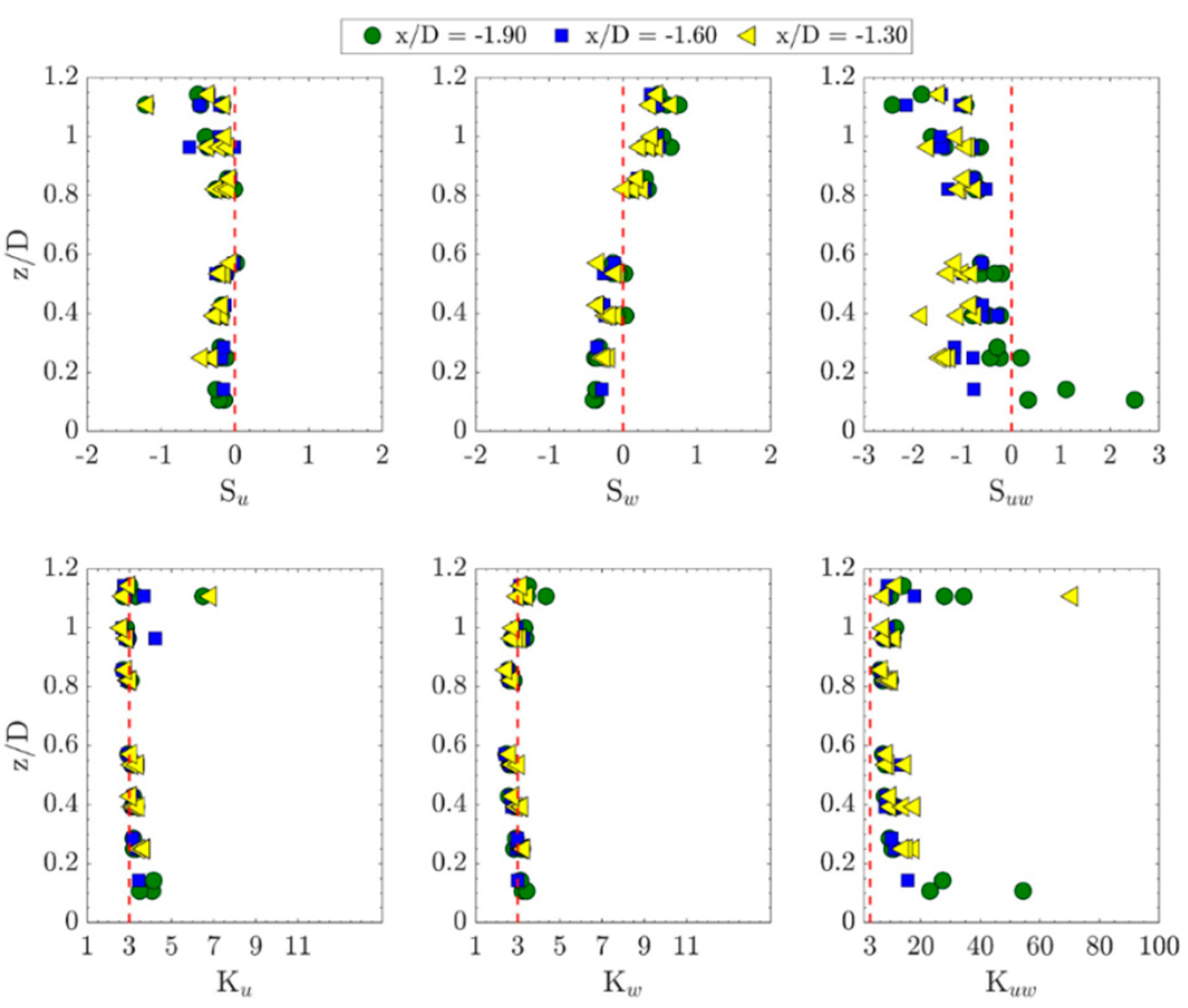
Figure 3.
Vertical profiles of the higher-order moments of velocity fluctuations downstream of the boulder.
Figure 3.
Vertical profiles of the higher-order moments of velocity fluctuations downstream of the boulder.

Figure 4.
Vertical profiles of the higher-order moments of velocity fluctuations at the sides of the boulder.
Figure 4.
Vertical profiles of the higher-order moments of velocity fluctuations at the sides of the boulder.

Figure 5.
Variation of the normalized streamwise integral length scale with the relative flow depth (normalized by boulder diameter) upstream of the boulder.
Figure 5.
Variation of the normalized streamwise integral length scale with the relative flow depth (normalized by boulder diameter) upstream of the boulder.
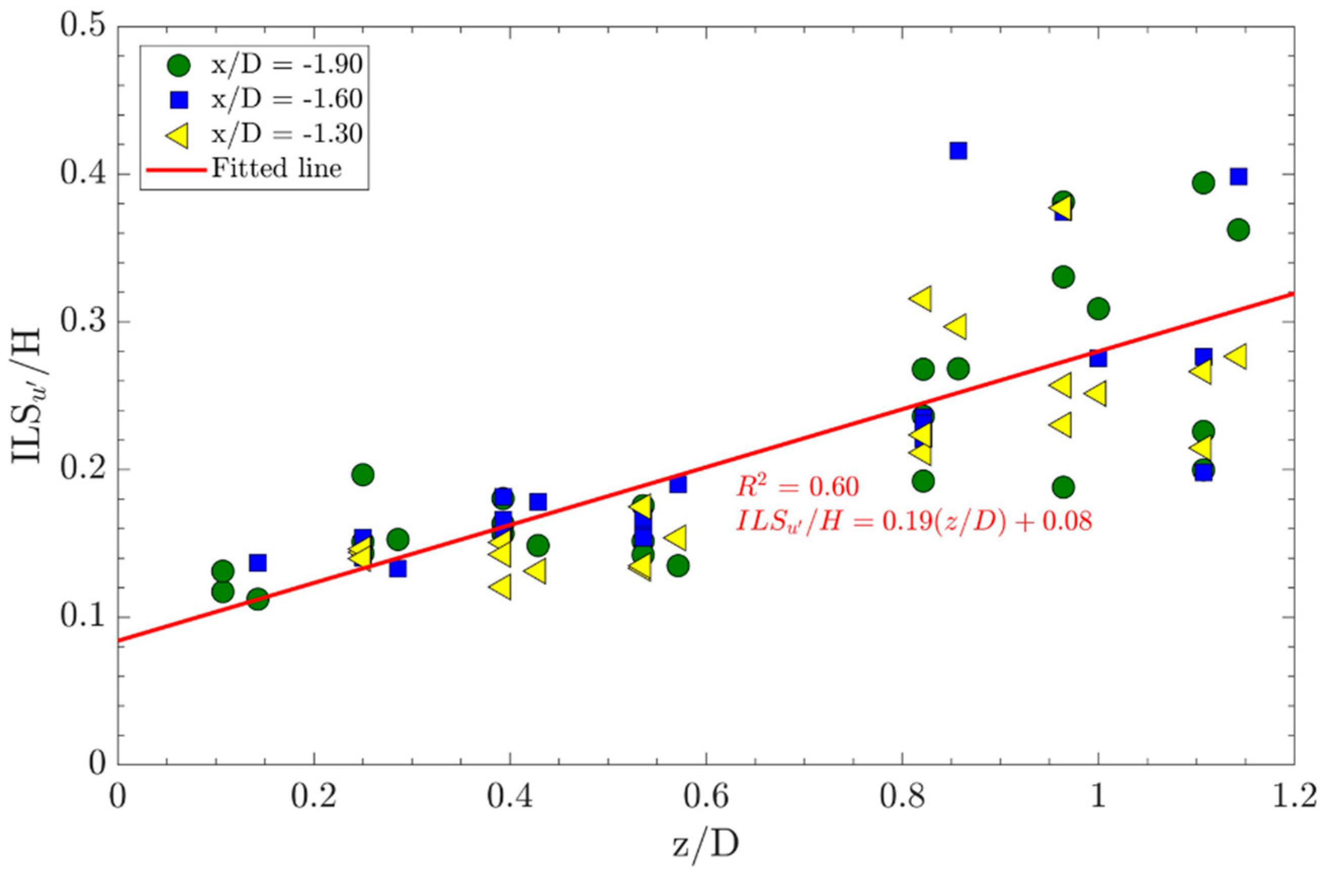
Figure 6.
Variation of the normalized streamwise integral length scale with the relative flow depth (normalized by boulder diameter) downstream of the boulder.
Figure 6.
Variation of the normalized streamwise integral length scale with the relative flow depth (normalized by boulder diameter) downstream of the boulder.

Figure 7.
Variation of the normalized streamwise integral length scale with the relative flow depth (normalized by boulder diameter) at sides of the boulder.
Figure 7.
Variation of the normalized streamwise integral length scale with the relative flow depth (normalized by boulder diameter) at sides of the boulder.
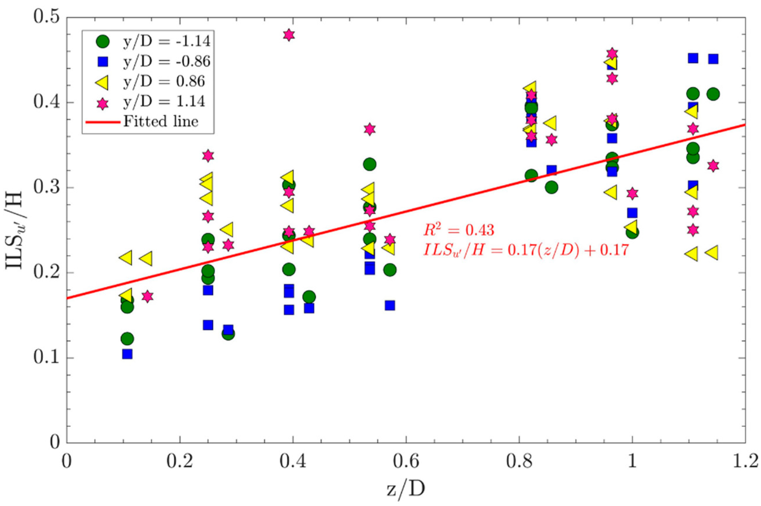
Figure 8.
Variations of the normalized energy dissipation rate (left) and normalized Kolmogorov’s length scale (right) over the flow depth upstream of the boulder.
Figure 8.
Variations of the normalized energy dissipation rate (left) and normalized Kolmogorov’s length scale (right) over the flow depth upstream of the boulder.

Figure 9.
Variations of the normalized energy dissipation rate (left) and normalized Kolmogorov’s length scale (right) over the flow depth downstream of the boulder.
Figure 9.
Variations of the normalized energy dissipation rate (left) and normalized Kolmogorov’s length scale (right) over the flow depth downstream of the boulder.

Figure 10.
Variations of the normalized energy dissipation rate (left) and normalized Kolmogorov’s length scale (right) over the flow depth at the sides of the boulder.
Figure 10.
Variations of the normalized energy dissipation rate (left) and normalized Kolmogorov’s length scale (right) over the flow depth at the sides of the boulder.
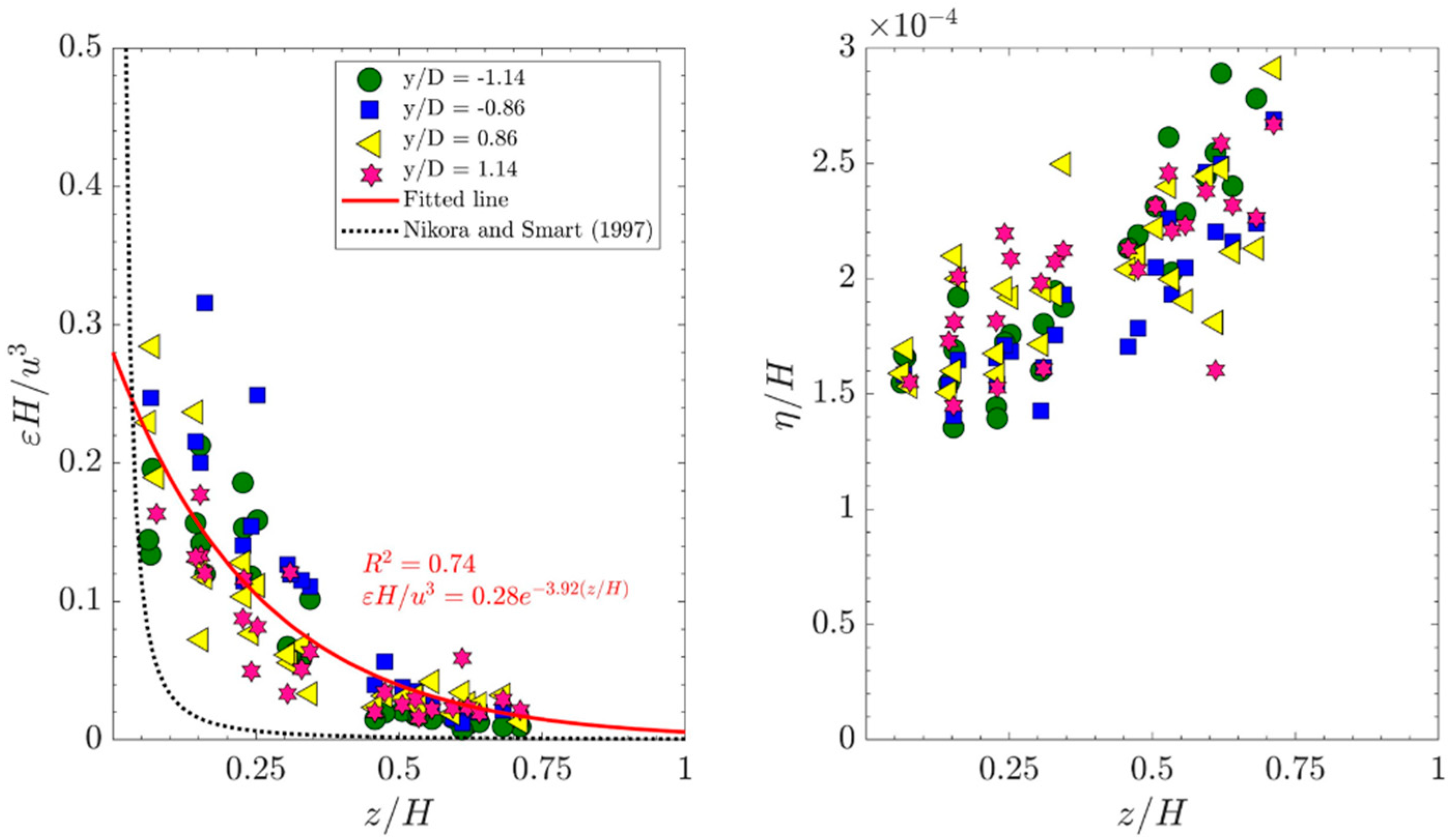
Figure 11.
Variation of the integral length scales around the boulder for (a) the model, and (b) the prototype. Integral length scale thresholds that may affect the swimming of a 200 mm body-length have been shown on the plots
Figure 11.
Variation of the integral length scales around the boulder for (a) the model, and (b) the prototype. Integral length scale thresholds that may affect the swimming of a 200 mm body-length have been shown on the plots

Figure 12.
Variation of EDF around the boulder for (a) the model and (b) the prototype. Minimum and maximum EDF thresholds for different fish species have been shown on the plots.
Figure 12.
Variation of EDF around the boulder for (a) the model and (b) the prototype. Minimum and maximum EDF thresholds for different fish species have been shown on the plots.


Table 1.
Variations of energy dissipation rate, Kolmogorov’s length scale and integral scale parameters around the boulder.
Table 1.
Variations of energy dissipation rate, Kolmogorov’s length scale and integral scale parameters around the boulder.
| Region | Upstream | Downstream | Sides | |||
|---|---|---|---|---|---|---|
| Parameter | Mean | Standard Deviation | Mean | Standard Deviation | Mean | Standard Deviation |
| 0.16 | 0.10 | 0.11 | 0.16 | 0.08 | 0.07 | |
| 0.00017 | 0.00002 | 0.00020 | 0.00003 | 0.00019 | 0.00003 | |
| ITSu’ [s] | 0.056 | 0.017 | 0.101 | 0.035 | 0.067 | 0.016 |
| ITSv’ [s] | 0.047 | 0.013 | 0.055 | 0.016 | 0.043 | 0.016 |
| ITSw’ [s] | 0.046 | 0.010 | 0.052 | 0.014 | 0.048 | 0.012 |
| ILSu’/H | 0.210 | 0.081 | 0.415 | 0.174 | 0.288 | 0.087 |
| ILSv’/H | 0.014 | 0.037 | 0.012 | 0.019 | 0.016 | 0.022 |
| ILSw’/H | 0.013 | 0.007 | 0.022 | 0.021 | 0.013 | 0.008 |
© 2020 by the authors. Licensee MDPI, Basel, Switzerland. This article is an open access article distributed under the terms and conditions of the Creative Commons Attribution (CC BY) license (http://creativecommons.org/licenses/by/4.0/).
Share and Cite
MDPI and ACS Style
Golpira, A.; Baki, A.B.; Zhu, D.Z. Higher-Order Velocity Moments, Turbulence Scales and Energy Dissipation Rate around a Boulder in a Rock-Ramp Fish Passage. Sustainability 2020, 12, 5385. https://doi.org/10.3390/su12135385
AMA Style
Golpira A, Baki AB, Zhu DZ. Higher-Order Velocity Moments, Turbulence Scales and Energy Dissipation Rate around a Boulder in a Rock-Ramp Fish Passage. Sustainability. 2020; 12(13):5385. https://doi.org/10.3390/su12135385
Chicago/Turabian StyleGolpira, Amir, Abul BM Baki, and David Z. Zhu. 2020. "Higher-Order Velocity Moments, Turbulence Scales and Energy Dissipation Rate around a Boulder in a Rock-Ramp Fish Passage" Sustainability 12, no. 13: 5385. https://doi.org/10.3390/su12135385
Note that from the first issue of 2016, this journal uses article numbers instead of page numbers. See further details here.