Article

CMIP5-Based Spatiotemporal Changes of Extreme Temperature Events during 2021–2100 in Mainland China

1
Laboratory of Geographical Processes and Ecological Security in Changbai Mountains, Ministry of Education, School of Geographical Sciences, Northeast Normal University, Changchun 130024, China
2
Urban Remote Sensing Application Innovation Center, School of Geographical Sciences, Northeast Normal University, Changchun 130024, China
3
Jilin Provincial Center of Land and Resource Information, Department of Natural Resources of Jilin Province, Changchun 130024, China
*
Author to whom correspondence should be addressed.
Sustainability 2020, 12(11), 4418; https://doi.org/10.3390/su12114418
Submission received: 26 March 2020 / Revised: 19 May 2020 / Accepted: 20 May 2020 / Published: 28 May 2020
(This article belongs to the Section Social Ecology and Sustainability)

Abstract

:
The increasing number of extreme climate events is having a great impact on the terrestrial ecosystem. In this study, we applied a Taylor diagram to evaluate the 7 extreme temperature indices (ETI) of 12 models and the multi-model ensemble (MME) mean from phase 5 of the Coupled Model Intercomparison Project (CMIP5) during 1961–2005, and found that the MME has the best simulation effect. Warm indices and warm duration indices increase slowly, rapidly, and extremely under the representative concentration pathway 2.6 (RCP2.6), RCP4.5, and RCP8.5 scenarios, respectively. In contrast, the decrease in cold indices and cold duration indices are slow, rapid and extreme, respectively. The ETI from 2021–2100 under the RCP2.6 and RCP4.5 scenarios have primary periods ranging from 1–16 years. Under the RCP2.6 and RCP4.5 scenarios, the changes of warm indices are relatively largest in the basin of the central, and southeastern, while, under the RCP8.5 scenario, the changes are relatively significant, except for basin of northeast. The cold indices have the most significant decreasing trend in the Tibetan Plateau and its surrounding areas, under the three RCP scenarios. The findings from this study can provide reference for the risk management and prevention of climate disasters in the context of climate change in mainland China.

1. Introduction

Due to its continuous and important impact on human health, ecosystem, social economy, industrial, and agricultural production, climate change has attracted extensive attention [1]. The Fifth Assessment Report of the Intergovernmental Panel on Climate Change (IPCC AR5) indicated that the earth system is undergoing a significant change, characterized by global warming from three different perspectives including observation, attribution analysis, and future prediction [2]. Climate change not only includes changes in mean climate, but also involves changes in extreme climate [3,4]. Furthermore, the extreme climate events, themselves, have a great impact on ecosystems, continuously changing the structure, function, and productivity of ecosystems, directly affecting the environment, as well as human living conditions, and the sustainable development of society [5,6], with an intensifying effect in future [2]. Therefore, in recent years there has been a high demand for understanding and simulating future extreme climate change [2,7,8]. The indices methods are used to study the changes in characteristics of extreme climate events. The most authoritative international extreme climate indices include the 27 extreme climate indices, defined by the Expert Team on Climate Change Detection and Indices (ETCCDI). The ETCCDI indices include 16 extreme temperature indices and 11 extreme precipitation indices [9], widely applied on the IPCC AR4 [10] and IPCC AR5 [2], reflecting changes in different aspects of extreme climate events.
The ETCCDI indices have been analysed by observation data [11], re-analyses data [12,13], and future climate modelling projections [14,15]. For instance, during the past 50 years, the number of cold nights has significantly decreased in more than 70% of the world’s land areas, while the number of warm nights has significantly increased [11]. In South America, extreme warm nights and days have significantly increased since 1950, revealing the characteristics of the overall climate warming in the region [16]. In the 20th century, a significant decrease trend was observed in the number of cold days and nights, with decrease rates of 3.7/10a and 6.0 days/10a, respectively, while, in some parts of Africa, the number of warm days and warm nights have significantly increased, at a rate of 8.2/10a and 8.6 days/10a, respectively [17,18]. The changes to such an extreme climate further intensify the process of aridity and desertification in the region, making the already bad ecological environment, worse. The frequency of extreme temperature events in China shows the same characteristics as the global, during 1961 to 2003, while, the increase is more pronounced in the northwest, northeast, and north China [1]. In the context of global warming, the frequency of extreme warm events is increasing, and the frequency of extreme cold events is decreasing on global, national and regional scales. Although, the same trend of extreme temperature events is observed in China and other regions around the world, the temporal and spatial changes of extreme temperature events show great regional characteristics. Therefore, it is necessary to carry out research on regional extreme temperature events.
In order to better identify data sharing and model comparison, the World Climate Research Program (WCRP) has started the Coupled Model Inter-comparison Project (CMIP), which has now progressed to the fifth stage (CMIP5) and serves as the global climate model for the IPCC AR5 key assessment [19]. The CMIP5 has provided the most extensive model database for climate model research, which includes 65 climate models from 14 countries, and can be used to study historical climates and predict future climate changes [19]. The external forces of future experiments are the representative concentration pathways (RCP) [20], including three commonly used scenarios, of RCP2.6, RCP4.5, and RCP8.5, which are widely used in studies across different fields [21,22]. The project results generally show that extreme climates increase with increasing radiative forcing, which means that cold (warm) extremes are greatly decreased (increased) in many regions of the world [7,23,24]. Nasrollahi et al. assessed the climatic drought conditions around the world based on the CMIP5, and suggested that most climate models overestimate the extreme drought in many regions [25]. Venkataraman et al. discussed the impact of climate change on drought characteristics in Texas (southern US), using the CMIP5 model. They concluded that the simulations had high reliability and stability [26]. You et al. calculated the extreme temperature indices of the Tibetan Plateau, based on 17 models of CMIP5 [27]. They ranked the simulation capabilities of each model, subsequently, four models with better simulation capabilities were selected to create the optimal model ensemble. However, so far, significant differences have been observed in the future extreme climate change simulated by different models under different RCP scenarios. Therefore, the simulation capabilities of each model must be ranked in order to select the best model for simulating future regional extreme climate changes.
The Taylor diagram [28] has been identified as an effective method, having been widely used in recent years for model evaluation and verification [29,30]. This method can comprehensively display the standard deviations of multiple modes of multiple CMIP5s, the correlation coefficients with reference values, and the root mean square deviation on a two-dimensional graph, which can fully and clearly reflect the simulation capabilities of multiple modes [28]. The standard deviation reflects the degree of dispersion of multiple variables, the correlation coefficient indicates the similarity between the variable value and the reference value, and the root mean square error indicates the dispersion between the variable and the reference value, not just considering one statistic. The climate change is a non-linear dynamic process. Fortunately, the ensemble empirical mode decomposition (EEMD) performs signal decomposition, based on the time-scale characteristics of the data itself, that is, the local stationary processing without the need of setting any basis functions in advance, which is particularly suitable for processing non-linear and non-stationary time series [31,32], therefore it has been widely used in the extreme climate change research [33].
China’s mean temperature has significantly increased over the past half century [34,35] and the increasing frequency, intensity, and duration of extreme climate events have greatly affected the China’s living environment, economic development, and social stability [36]. Since the end of the last century, direct economic losses due to meteorological disasters, especially extreme climate events, have reached 300 billion yuan, accounting for 87% of all natural disasters [37]. During recent years, many researchers have studied the future changes of China’s extreme climate under different RCP scenarios. Based on multiple models of CMIP5, Zhou et al. suggested that the cold extremes (warm extremes) under the RCP4.5 and RCP8.5 scenarios have significantly decreased (increased), compared to the past few decades [38]. In fact, the extreme climate prediction process has multiple uncertainties, such as model structure, scale conversion, and emission scenarios, moreover, the climate change is a non-linear dynamic system. Therefore, it is necessary to evaluate the simulation effects of multiple models in order to select the best model or ensemble and apply the nonlinear trend analysis methods to reduce the uncertainty of future extreme climate predictions. This study aims to analyse the spatiotemporal characteristics of future extreme temperature events in mainland China, based on the CMIP5 multi-model. Furthermore, this study aims to provide useful information and accurate data on future climate change for policy makers to enable them to successfully adjust the strategies, in accordance with the climate change.

2. Data and Methods

2.1. Data

2.1.1. Observed Climate Data

The observed daily maximum and minimum temperature (Tmax and Tmin) dataset during the 1961–2005 is obtained from National Meteorological Information Center of the China Meteorological Administration. The dataset is based on the basic meteorological element data of more than 2400 national surface meteorological stations in China, which are newly compiled by the basic data project. Using the Thin plate spline (TPS) combined with 3D geospatial information for spatial interpolation, the daily temperature and precipitation grid data are established with spatial resolution rate of 0.5° × 0.5° since 1 January 1961 in China. Moreover, cross validation and error division are carried out to ensure good data quality. This dataset has been widely used in the study of extreme climate indices [39,40]. The entire mainland China is selected as the study area (Figure 1), where the annual mean temperature (Tmean) ranges between −12.3–25.3 °C. The Tmean in the Northeast and the Tibetan Plateau is lower than 0 °C, while, the other regions have a temperature higher than 0 °C. The numbers 1–9 in the Figure 1 refers to represent the 9 basins, in the study area.

2.1.2. CMIP5 Data

In this study, we used the 12 CMIP5 models (Table 1) obtained from The Earth System Grid Federation (ESGF, https://esgf-node.llnl.gov/projects/esgf-llnl/), including historical (1961–2005) and 21st century (2006–2100). The selected RCP2.6, RCP4.5, and RCP8.5 correspond to the low, medium, and high emission scenarios, respectively. The RCP2.6 is a low-emission greenhouse gas scenario and the radiative forcing in this scenario will increase to 3.1 W/m2 in the middle of the 21st century, followed by decreasing to 2.6 W/m2 by 2100. The RCP4.5 is a medium- emission scenario, in which the radiation intensity will reach 4.5 W/m2 by 2100. Finally, the RCP8.5 is a high-emission scenario, in which the greenhouse gas concentration will continue to increase throughout the period and the radiative forcing will reach 8.5 W/m2 by 2100 [20].

2.2. Methods

2.2.1. Extreme Temperature Indices

In this study, the observed daily climate data and CMIP5 data are used to calculate the 7 extreme temperature indices (ETI) that are recommended by the ETCCDI [9] (Table 2). The TX10p, TN10p, CSDI, and FD0 indicate the extreme low temperature events, and the TX90p, TN90p, and WSDI indicate the extreme high temperature events.

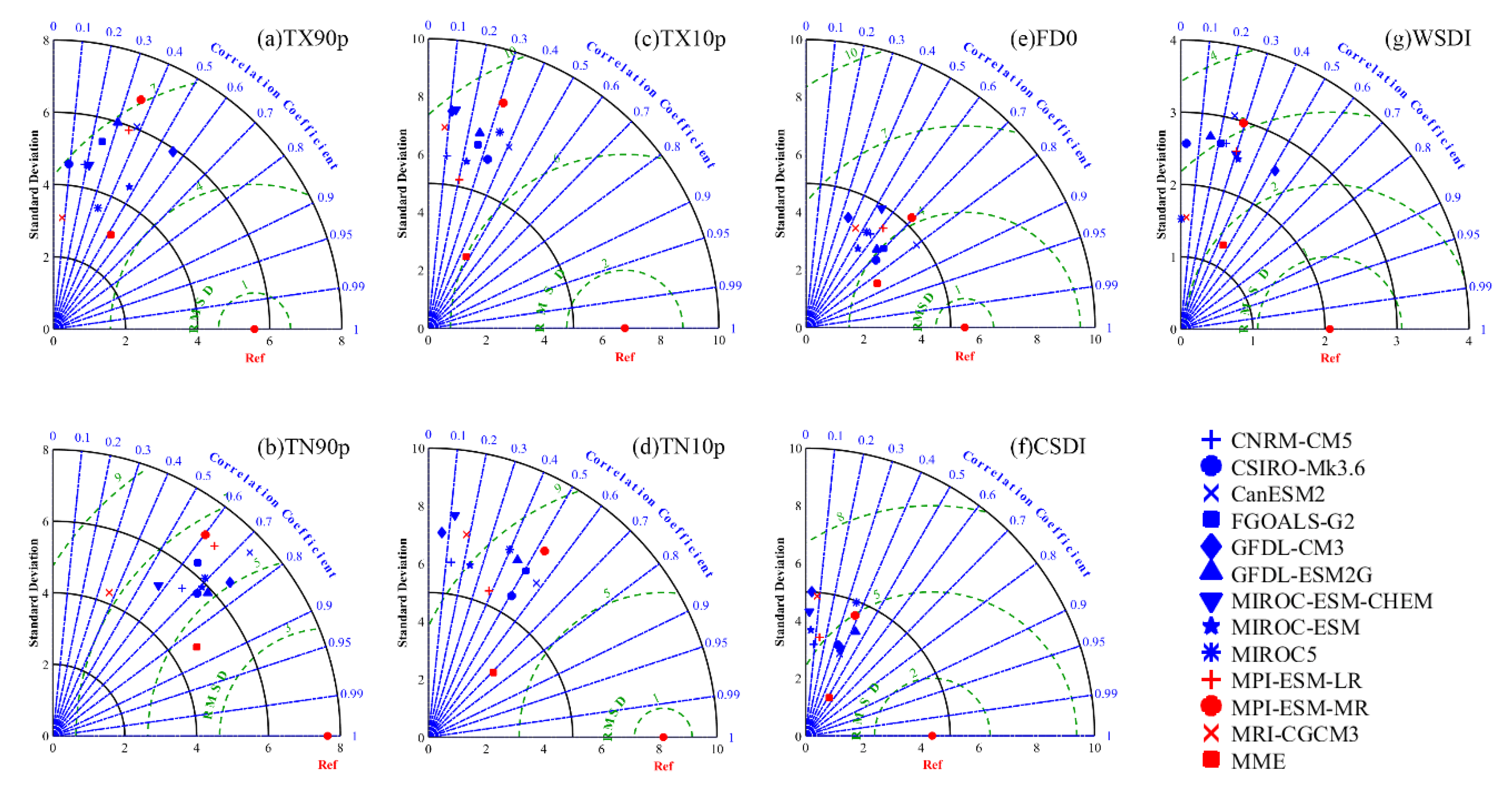
2.2.2. Taylor Diagram

In this paper, the Taylor Diagram [28] was used to evaluate the simulation effect that ETI from CMIP5 historical models on the true ETI. This method uses three statistics, correlation coefficient (R), standard deviation (STD), and root mean square error (RMSE) to quantify the difference between the simulated value of the model and the truth value. Assuming the observation data is O and the simulation capabilities of the two modes A and B need to be compared, we first should calculate the standard deviations σ O and σ O of O and A, respectively, R and RMSE for O and A. In Taylor diagram, the RMSE, σ A and R of O and A meet the following requirements:
R M S E 2 = σ O 2 σ A 2 2 σ O σ A R
The same method can calculate three statistics between B and the truth value. If a model is closer to the truth value, it means that the R of the model is high, the STD and RMSE are small, and the model is better than other models.

2.2.3. Ensemble Empirical Mode Decomposition

Ensemble empirical mode decomposition (EEMD) is based on the principle of measuring the average value multiple times [31]. By adding appropriate white noise to the original data, the EEMD makes the signal to have continuity on different scales. At the same time, the added white noise is aggregated after multiple calculations, and it is an improvement of empirical mode decomposition [41]. In this study the EEMD is used to analyse the temporal changes of the ETI in mainland China, under different RCP scenarios in future (2021–2100). The amplitude of the added noise is set to 0.25 [32]. First, add a white noise series to the original data:
x i ( t ) = x ( t ) + n i ( t ) ,
where, x i is the new signal, obtained by adding the ith white noise to the original signal data ( t ) , and n i ( t ) is the white noise. Second, find out all local maxima and minima of x i ( t ) , use the cubic spline interpolation method to form the upper envelope ( u 1 ( t ) ) and the lower envelope ( u 2 ( t ) ), subsequently, the local mean envelope can be calculated, as follows:
m 1 ( t ) = 1 2 ( u 1 ( t ) + u 2 ( t ) )
The interpolation of x i ( t ) and m i ( t ) is the series h :
h 1 ( t ) = ( x i ( t ) m 1 ( t ) )
After k repetitions, we get h 1 k ( t ) that meets the requirements of the Intrinsic Mode Function (IMF), that is, the first IMF:
h 1 k ( t ) = h 1 ( k 1 ) ( t ) m 1 k ( t )
Re-add a new white noise series and repeat the above steps to add the IMF, obtained each time, to perform the integrated average processing to acquire the final decomposition result. The result includes both multiple IMF components and a trend term, and this study selected the trend item.

2.2.4. Continuous Wavelet Transform

Continuous wavelet transform (CWT) can reveal the multiple periodic changes, hidden in the time series, in order to fully reflect the changing characteristics of variables in different time scales [42]. In this study, the Morlet continuous wavelet is applied to analyse the periodic change of ETI from 2021–2100, as follows:
ψ ( t ) = π 1 / 4 e i ω 0 η e η 2 / 2 ,
where, ω 0 and η are dimensionless frequency coefficients and time series, respectively. Generally, ω 0 = 6 can well balance the time-frequency domain. The continuous wavelet processing of the data X n ( n = 1 , 2 , , N ) is mainly performed by convolution and scale transformation processing ψ 0 ( η ) :
W n ( s ) = n N 1 x n ψ [ ( n n ) δ t s ] ,
where, * represents a complex conjugate function, N is a time series, n is a time conversion index, n is a local time index, and ψ is a normalized wavelet variation. The wavelet transform is based on the assumption that the data is cyclic. Therefore, when dealing with a finite-length time series, the edge effects appear in the wavelet power spectrum, that is, errors occur at the start and end of the power spectrum. Cone of influence (COI) [42,43] represents the wavelet power spectrum region and the corresponding edge effect, which decreases e 2 with the edge wavelet power spectrum | W n ( s ) | 2 .

2.2.5. Sen′s Slope + Mann-Kendall Test

In the trend analysis of long time series, Sen‘s slope has been used to detect the magnitude of the changes, which can effectively avoid the interference of outliers [44]. The formula is as follows:
β = m e d i a n ( x j x i j i ) ,     1 < i < x < j ,
where, x i and x j represent the values of the i th and j th years in the time series, respectively. When β < 0, it indicates a decrease trend, and vice versa. The Mann-Kendall (MK) non-parametric test does not require time series data to follow a normal distribution, and the results are not affected by outliers [45]. In this study, the Sen’s slope and the MK test are combined to analyse the spatial changes of future ETI.

3. Results

3.1. Performances of Models

Based on the ETI, calculated from the observation data from 1961 to 2005 and applying the Taylor diagrams, we evaluate the ETI, calculated from the 12 CMIP5 models and the multi-model ensemble (MME) mean, subsequently, the future climate models are selected that are most suitable for different ETIs in mainland China (Figure 2). The results show that a considerable difference in simulated ETI is observed in different models. For the TX90p (Figure 2a), most models have the STDs between 2–6, the Rs between 0.5–0.8, and the RMSDs between 4–7. For the TN90P (Figure 2b), the R of MME has reached 0.83, and both the SD and the RMSD are small. For the cold indices (TX10p, TN10p, and FD0), compared to the most models, the simulation results of MME are far superior to other models (Figure 2c–e), especially the correlation coefficient is higher than that of any single model. For the duration indices (CSDI and WSDI), still the MME has the highest correlation, and the STD and the RMSE are the smallest (Figure 2f,g). In general, the simulation of MME is closest to the truth value, and consistently shows better performance than all individual models for all ETI. In this study, we only analysed the temporal and spatial changes of MME from 2021–2100.

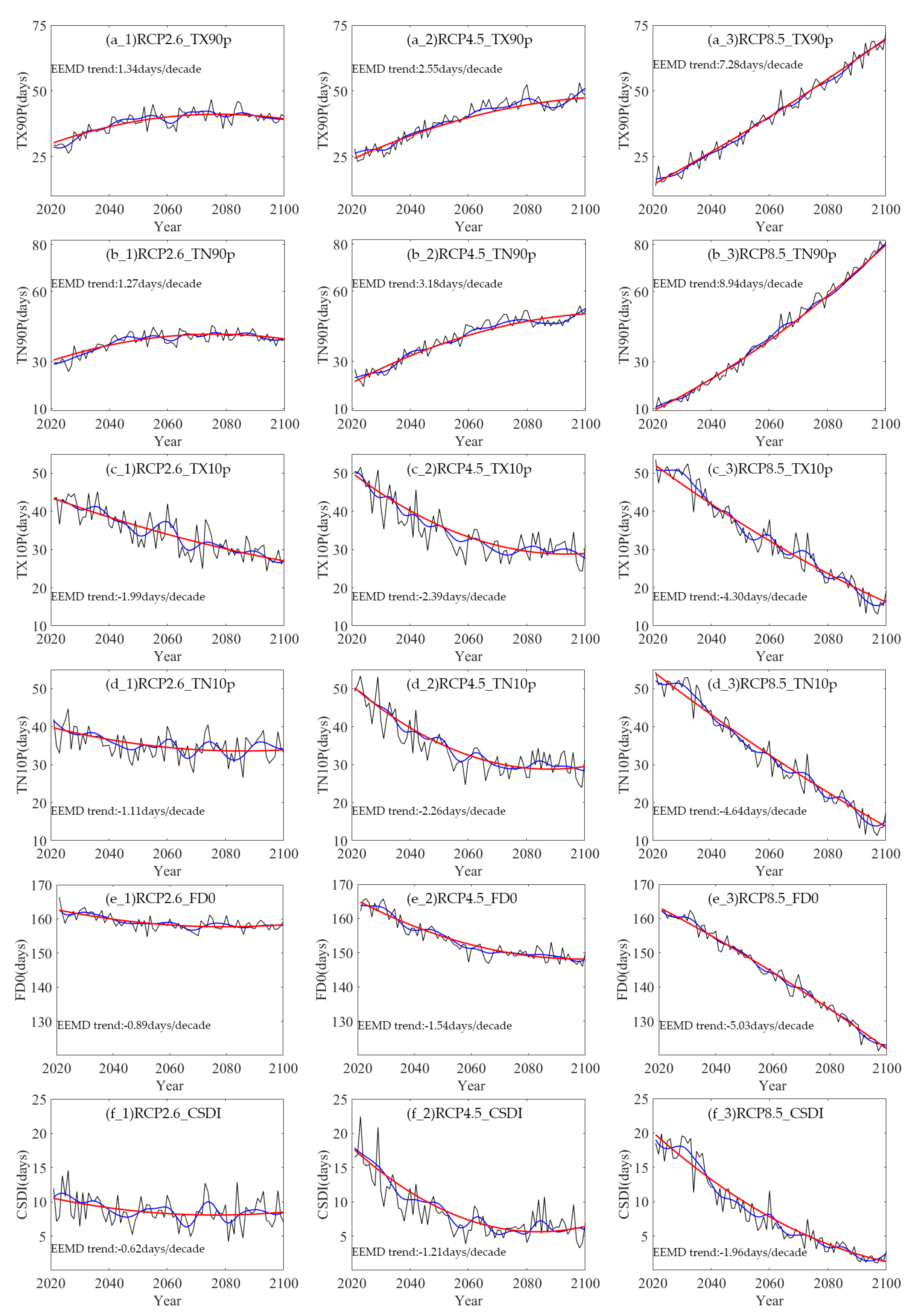
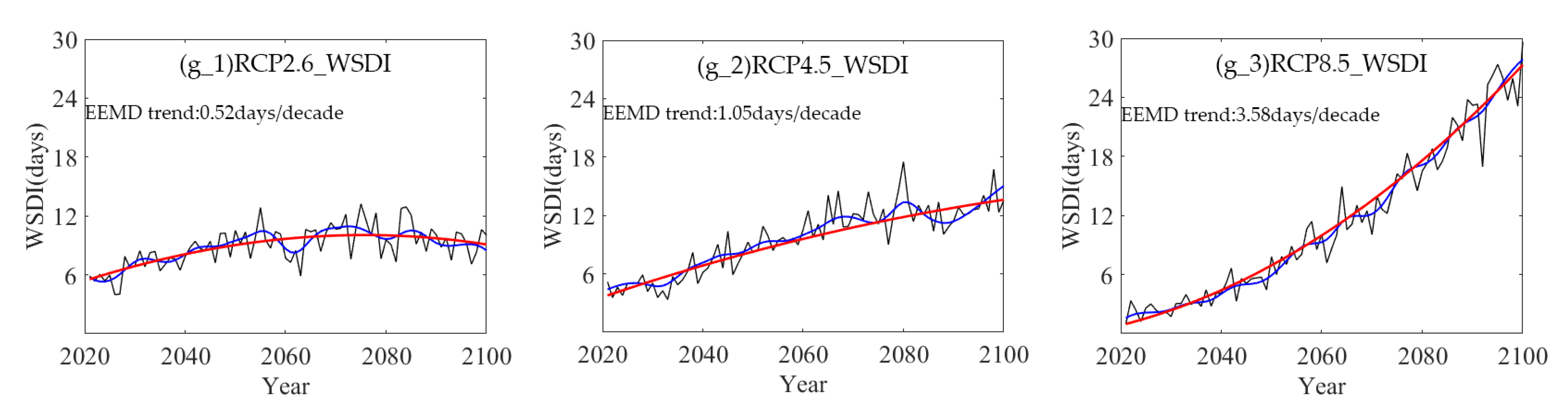
3.2. Future Temporal Changes of ETI

The EEMD method is used in this study to analyse the trends of 7 ETIs under different RCP scenarios. From 2021 to 2100, the EEMD trends of TX90p in the RCP2.6, RCP4.5, and RCP8.5 are 1.34 days/decade, 2.55 days/decade, and 7.28 days/decade, respectively (Figure 3a_1–a_3). Under the RCP2.6 scenario, there will be a slight increasing trend before 2070, and the trend will become slowly decreasing after 2070. Under the RCP8.5 scenario, an extremely fast increasing trend is expected, reaching the highest value in 2100 (72.1 day). For the TN90p, the trends in RCP2.6, RCP4.5, and RCP8.5 are 1.27 days/decade, 3.18 days/decade, and 8.94 days/decade, respectively (Figure 3b_1–b_3). Under the RCP2.6 scenario before 2060, a significant increasing trend is identified in the TN90p, followed by an slightly decreasing trend. Moreover, under the RCP4.5 scenario, the period before 2080 is expected to experience an increasing trend, after which it almost enters a stagnant state. Under the RCP8.5, a rapid increase is identified, reaching 81 days by 2100. The cold indices (TX10p, TN10p, and FD0) show the smaller changes in the RCP2.6 scenario, with a generally decreasing trend. While, in the RCP4.5 scenario, the cold indices decrease rapidly before 2080, after which the slight changes are expected and the EEMD trend is −2.39 days/decade, −2.26 days/decade, and −1.54 days/decade, respectively. Furthermore, under the RCP8.5 scenario, the cold indices show an extreme decreasing trend, with the EEMD values of −4.3days/decade, −4.64 days/decade, and 5.03 days/decade, and the lowest values appear after 2094, which are 13.07 days, 11.32 days, and 121.25 days (Figure 3c_1–e_3). Under the RCP2.6 scenario, the CSDI showed a decrease and then stagnation, with a turning time of 2060; in the RCP4.5 scenario, it shows a rapid decrease, followed by an slow increase, with a turning time of 2080. Under the RCP8.5 scenario, an extremely decreasing trend is identified (Figure 3f_1–f_3). Finally, under the RCP2.6 scenario, the WSDI will increase gradually by 2060 and then stagnate, while, in both RCP4.5 and RCP8.5 scenarios, an obvious increasing trend is identified (Figure 3g_1–g_3). In addition, the rate of change of TX90p, TX10p, and WSDI in any RCP scenario is greater than the historical period (19961–2005, Figure S1a,c,g). Under the RCP4.5 and RCP8.5 scenarios, the rate of change of TN90p and TN10p is greater than the historical period (Figure S1b,d). The decrease rate of FD0 and CSDI is greater than that of historical period, under the RCP835 scenario (Figure S1e,f).

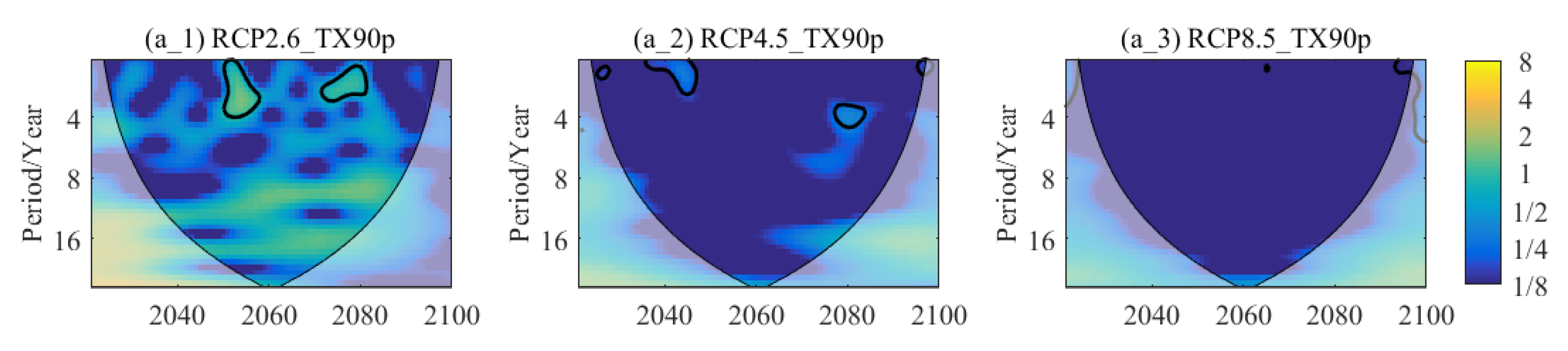
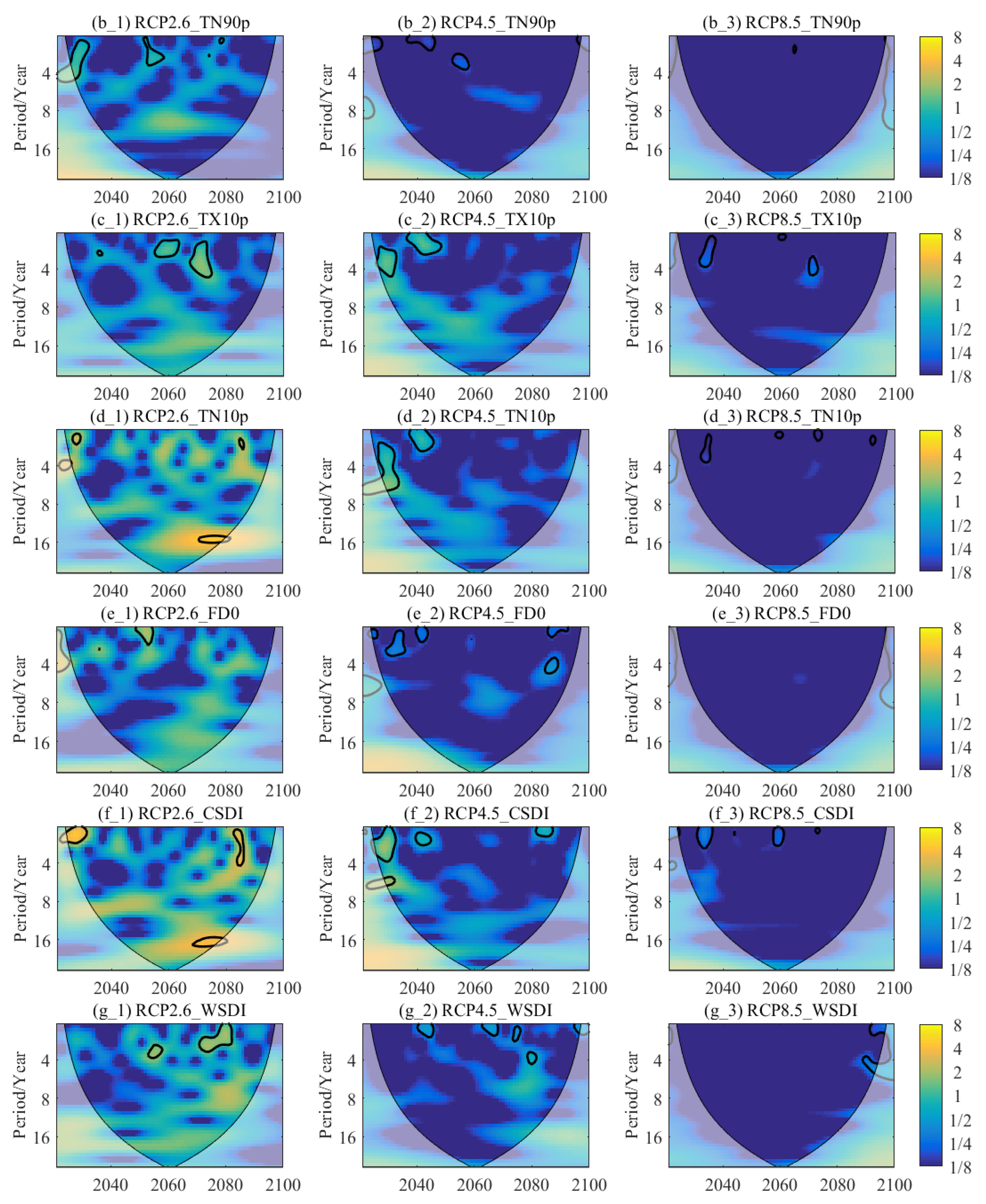
3.3. Future Periodic Oscillation of ETI

In this study, the Morlet CWT is applied to perform periodic analysis of the ETI under different RCP scenarios, in mainland China from 2021–2100. The primary period of each ETI can be read from the colour bar of the wavelet map, that is, the period of maximum vibration intensity. As it can be seen from Figure 4, under the RCP2.6 scenario, the primary periods of the TX90p, TN90p, TX10p, TN10p, FD0, CSDI and WSDI are 10, 10, 16, 16, 16, 16, and 8 years (the first column in Figure 4). Under the RCP 4.5 scenario, the primary periods of these indices are 2, 2, 10, 10, 4, 7, and 8 years (the second column in Figure 4). Finally, in the RCP8.5 scenario, the primary periods of the TX10p and CSDI were 4 and 2 years (the third column in Figure 4). The primary periods from 1961 to 2005 were 4, 4, 6, 8, 8, 8, and 6 years, respectively (Figure S2a–g).
In different time periods, under the RCP2.6 scenario (the first column of Figure 4), the TX90p shows a significance 4 years periods fluctuation from 2050–2058, and a 1–3 years periods fluctuation from 2070–2080. Under the TN90p has significant periods of 1–5 and 1–3 years in 2021–2030 and 2052–2059, respectively. Moreover, the TX10P shows 1–5 years significant periods change in 2056–2076, while, the TN10p in 2025–2028 and 2070–2080 have significant period of 2 and 16 years, respectively. The FD0 has significant periods of 1–3 years between 2052–2056. The CSDI has significant periods of 2 and 16 years between 2022–2030 and 2066–2080, respectively. The WSDI has significant periods of 3 and 1–3 years between 2054–2056 and 2070–2080, respectively. Under the RCP4.5 scenario (the second column of Figure 4), the TX90p has significant periods fluctuations of 3 and 3–4 years between 2038–2048 and 2078–2082, respectively. The TN90p has significant periods of 2 and 2–4 years between 2038–2046 and 2056–2060, respectively, while, the TX10p has significant periods of 1–5 years between 2025–2048. Moreover, under the same scenario, the TN10 has significant periods of 2–7 and 1–3 years between 2025–2032 and 2038–2046, respectively, while, the FD0 has significant periods of 1–3 and 4 years between 2022–2042 and 2086–2091, respectively. The CSDI has significant periods of 1–6 and 2 years between 2024–2044 and 2081–2086, respectively, while, the WSDI has significant periods of 4 years 2078–2082. Under the RCP8.5 scenario (third column of Figure 4), the TX10p, TN10p, and CSDI have shorter significant periods, and other ETIs have no significant periodic fluctuations.

3.4. Future Spatial Changes of ETI

The spatial distribution of the trends of ETI in mainland China under different RCP scenarios from 2021–2100 is presented in Figure 5. As presented in figure, the warm indices, cold indices and duration indices of the entire mainland China show the same change trend under three RCP scenarios, however, the change range for each scenario are different. Under the RCP2.6 and RCP4.5 scenarios, the increase trends of warm indices (TX90p and TN90p) in Haihe River basin, Huaihe River basin, Yangtze River basin, Pearl River basin, and Southeast basin is relatively large (Figure 5a_1,2 and b_1,2). Under the RCP8.5 scenario, except for Songhua and Liaohe River basin, in most areas of the Yellow River basin and the eastern part of the Continental Basin, the increase trend is larger and the area with the most changes is located in the Pearl River basin (Figure 5a_3 and b_3). In the past (1961–2005), a significant increase was identified, except for the central region, especially in the continental basin, as well as the Songhua and Liao He River basin (Figure S3a,b). For the TX10p (TN10p), under the RCP2.6, RCP4.5, and RCP8.5 scenarios, the Tibetan Plateau area has the fastest decrease rates, with the highest decrease rates of −0.42 (−0.24), −0.47 (−0.47), and −0.79 (−0.84), while, the decrease rate is more uniform in other areas (Figure 5c_1–c_3 and d_1–d_3). The northern region experienced significant changes in the past (Figure S3c,d). The FD0 in all three scenarios has a large change in most areas of the Yangtze River basin, Southwest basin, Yellow River basin, and Continental basin, and the smallest change occurs in Pearl River basin and Southeast basin (Figure 5e_1–e_3). The FD0 had considerable change in the continental basin during the historical period (Figure S3e). For the duration indices (CSDI and WSDI), the both trends and areas are opposite. Under the RCP2.6 scenario, the CSDI shows a larger decrease rate in the Yangtze River basin, Pearl River basin, Southeast basin, and Southwest basin regions (Figure 5f_1). Under the RCP4.5 and RCP8.5 scenarios, the changes in the middle of the Yellow River basin, the middle of the Yangtze River basin, the middle of the Continental basin, and the Southwest basin are relatively large, and the maximum trends in the Southwest basin are −0.25days (RCP4.5) and −0.44 (RCP8.5), respectively (Figure 5f_2,3). Under the three RCP scenarios, the WSDI has the largest increasing trend in the southeast, west, and northwest, with the maximum trends of 0.24, 0.4, and 0.68 days (Figure 5g_1–g_3). The decrease (increase) of The CSDI (WSDI) in the continental basin and northern China is most significant in the past (Figure S3f,g).

4. Discussion

Climate change, dominated by warming over the past century, has had a significant impact on the frequency, intensity, spatial extent, and duration of the extreme climate events [2]. This phenomenon will continue to increase globally in the future, based on the CMIP5 model [46,47,48]. Among the 12 CMIP5 models and MMEs that we initially selected, the MME is far superior to all single models for simulating the ETI, and the results are consistent with previous studies [14,49]. Therefore, we project the spatiotemporal changes of ETI in future of China (2021–2100) based on the MME.
The EEMD method, applicable to the non-linear change, is applied to analyse the temporal changes of ETI in mainland China during 2021–2100, under different RCP scenarios. Based on the results, most ETIs have turning years under different RCP scenarios, a non-linear trend. Based on our findings, under the three RCP scenarios the warm indices (TX90p and TN90p) are increasing and the change in TN90P is greater than TX90p, indicating that in any future scenario, the increase in warm night-time is greater than warm day-time. It also shows that this phenomenon, which has happened in the past (Figure S1a,b) will continue in the future, but the increase difference between the TX90p and TN90p is smaller than that in the past, under the three future RCP scenarios. For the cold indices (TX10p and TN10p), a decreasing trend is observed under all RCP scenarios. The decrease of TN10p is greater than TX10p, under the RCP8.5 scenario, which is consistent with the past phenomena (Figure S1c,d). However, based on our findings, under the RCP2.6 and RCP4.5 scenarios, the decreasing rate of TX10p is greater than the TN10p, that is, the cold day-time is greater than the cold night-time, which indicates that the past trend will be changed in future. Furthermore, the has FD0 decreased at a rate of 1.8 days per 10 years during the period 1961–2005 in mainland China (Figure S1e). However, in the next 80 years, the decreasing rate of FD0 is greater than that of the past changes under the RCP8.5 scenario, and the decreasing trend is 2.79 times the past (−5.03 days per 10 years). The changes in the RCP2.6 and RCP4.5 scenarios are less than that of the past changes. Under the RCP2.6 and RCP4.5 scenarios, the decrease rate of the CSDI is greater than the increase rate of the WSDI, which maintains the past phenomenon (Figure S1f,g), however, the change difference is smaller, compared to the past. In general, the 7 ETIs, calculated by the MME, show great differences in the degree of change under different RCP scenarios. The change is slow in the RCP2.6 scenarios, rapid in the RCP4.5 scenarios, and extreme in the RCP 8.5 scenarios, and these changes are similar to trends of ETIs in global [8] and China [50].
The changes in extreme climate indices are not only complex and diverse, but also appear as multi-frequency and quasi-periodic time-domain vibrations. Li et al. analysed future projections of ETIs in sub-regions of China and found out the periodicity in the RCP4.5 scenario is stronger, in comparison with the RCP8.5 [51]. In this study, we not only analysed the periodicity of ETI under the RCP4.5 and RCP8.5 scenarios, but also analysed the periodicity in the RCP2.6 scenario. We discovered that all ETI have strong periodicity under the RCP2.6 scenario, with RCP4.5 being the second, while it was the least significance in under the RCP8.5 scenario. This result related to the slow changes of ETIs under the RCP2.6 scenario, which causes a significant periodic between different years. However, under the RCP8.5 scenario, the changes of ETIs either increases extremely or decreases extremely, and the changes might be the reason of making the period of ETI longer and insignificant. The latter suggests that in the future, mainland China should take farther preventive actions in the years when the ETI has significance periods fluctuation. In addition, the past primary period (Figure S2) of the ETI is smaller than the three RCP scenarios in the future, which can be due to the different years of application.
For spatial changes, under the different RCP scenarios, the ETIs changes in various basin are different. For the warm indices, under the RCP2.6 and RCP4.5 scenarios, the changes in the basin of east and southeast are relatively largest, especially in the Pearl River basin. For the cold indices, the changes in the west are more prominent under the three RCP scenarios, especially the Tibetan Plateau and the surrounding area. However, during 1961–2005, the warm index changed the most in the western and northern basins (Figure S3a,b), while, the cold index changed the most in the northern and north-eastern basins (Figure S3c,d), indicating that the regions with the greatest changes in the warm index and cold index in the future will change, hence, such regions should pay more attention to preventive actions. Regarding the FD0, whether in the past or in the future, the largest changes have been observed in the Tibetan Plateau region (Figure S3e). Therefore, object that are more affected by the FD0 in the Tibetan Plateau should be strengthened. The duration indices are more prominent in the basin of southeast, west, and northwest, which is opposite of the areas with large changes in the past (Figure S3f,g). The changes in the ETIs in the Songhua and Liaohe river basin are relatively small in future, probably due to presence of large forests in this area [52], therefore, the impact of climate change is relatively small. In general, compared to the past, the area with greater changes in the ETI will increase in the future, indicating that the affected area is increasing. In the past, the changes in the ETI in the west and north of China were relatively large. However, in the future, under different RCP scenarios, the changes in the east and southeast will be greater compared to the other regions. The results from our study shows that the frequency, intensity, and duration of ETIs in mainland China will increase in future, regardless of the type of the emission scenario (RCP2.6, RCP4.5 and RCP8.5), which will have a certain negative impact on the ecological environment and residents’ lives. The residents and stakeholders should adjust to reduce the losses, caused by ETIs.
Some uncertainties are identified in our study. Firstly, although there are more than 60 models in CMIP5, we only applied 12 models that exist in history, under the RCP 2.6, RCP 4.5 and RCP 8.5 scenarios with the same year, which may also reduce the accuracy of the MME. Secondly, each model is produced in different organizations, and the resolution is not the same. In order to match the model with the observation data, the spatial resolutions of all models were resampled to 0.5° × 0.5°, which to some extent overestimates or underestimates the mean of ETIs in mainland China.
Through this study, we have verified that the ETI frequency and intensity have been increased in different regions of mainland China, over the past few decades [33,53,54,55]. Most areas of mainland China have experienced a half-century drought, which has had a significant impact on vegetation dynamics [56,57], phenology [58,59,60], hence, causing a large economic loss [37]. The results from our study show that this phenomenon in mainland China will continue at least until the end of the 21st century, regardless of the RCP scenario. Therefore, effective measures should be taken in mainland China, such as planting trees and afforestation, reducing felling, and increasing environmental awareness among people in order to avoid or mitigate more losses, caused by future extreme climate events and to protect natural resources and human health. In future, we will apply more climate simulation models and impose the downscaling method to project future spatial and temporal trend of extreme climate events in mainland China and to quantify the impact of extreme climate events on vegetation and ecological environment.

5. Conclusions

In this study, based on the 7 ETI, calculated from the observed daily maximum and minimum temperature data of mainland China in 1961–2005, we applied Taylor diagram to evaluate the 7 ETI of 12 models and MME mean from the CMIP5 during 1961–2005. At the same time, the model with the best simulation effect were selected to predict the spatiotemporal changes of the ETI in mainland China in 2021–2100.The main findings of our study are, as follows:
(1)
For the 12 models that simulate 7 ETIs, the MME has the best simulation effect, compared to the single model.
(2)
For the future temporal changes of the ETI, the warm indices (i.e., the TX90p and TN90p) and the WSDI increase slowly under the RCP2.6 scenario, rapidly under the RCP4.5 scenario, and extremely under the RCP8.5 scenario. In contrast, the decrease of cold indices (i.e., the TX10p, TN10p, and FD0) and the CSDI under the RCP2.6, RCP4.5 and RCP8.5 scenarios are slowly, rapidly, and extremely, respectively.
(3)
For the future periodic oscillation of the ETI, the ETIs from 2021–2100 under the RCP2.6 and RCP4.5 scenarios have primary periods, ranging from 1–16 years, with the significance periodic of 1–4 years, but insignificance under the RCP8.5 scenario.
(4)
For the future spatial changes of the ETI, under the RCP2.6 and RCP4.5 scenarios, the changes of warm indices are relatively largest in the central and south-eastern basins. Under the RCP8.5 scenario, the changes are relatively large, except for northeast basin. The cold indices show the most significant decreasing trend in the Tibetan Plateau and its surrounding areas, under the 3 RCP scenarios. The decrease trend of the CSDI is the most significant trend in the central, a part of north-western, and the southwestern basins. The increase trend of the WSDI in the south-east and north-west of China is the largest and the most significant trend.

Supplementary Materials

The following are available online at https://www.mdpi.com/2071-1050/12/11/4418/s1, Figure S1: The historical (1961-2005) EEMD trends of (a) TX90p, (b) TN90p, (c) TX10p, (d) TN10p, (e) FD0, (f) CSDI, (g) WSDI in mainland China. The black lines represent the annual series of the ETI, the blue lines indicate the inter-decadal variation and the red lines represent the trend component, Figure S2: The historical (1961-2005) wavelet power spectrum of (a) TX90p, (b) TN90p, (c) TX10p, (d) TN10p, (e) FD0, (f) CSDI, (g) WSDI in mainland China The ‘V’-shaped black lines indicate the influence cone, the closed black lines represent the significant area at 95% confidence level, and the colour bars correspond to the vibration intensity of the periods at different timescales, Figure S3: The historical (1961-2005) spatial distribution of the trends of (a) TX90p, (b) TN90p, (c) TX10p, (d) TN10p, (e) FD0, (f) CSDI, (g) WSDI in mainland China. The black dots indicate the insignificant at 95% confidence level.

Author Contributions

All authors contributed meaningfully to this study. Conceptualization, H.Z. (Hongyan Zhang); Methodology, H.Y.; Software, H.Z. (Hang Zhao), X.G.; Validation, Z.Z., R.W.; Formal Analysis, H.Y.; Data Curation, J.Z., G.D.; Writing—Original Draft Preparation, H.Y.; Writing—Review & Editing, H.Z. (Hongyan Zhang); Supervision, Y.S. All authors have read and agreed to the published version of the manuscript.

Funding

This work was financially supported by the National Natural Science Foundation of China (Grant No. 41871330, 41771450 and 41761101), the Science and Technology Development Project of Jilin Province (Grant No. 20180623058TC and 20190802024ZG), foundation of the Education Department of Jilin Province in the 13th Five-Year project (Grant No. JJKH20170916KJ and JJKH20190282KJ), the Fundamental Research Funds for the Central Universities (Grant No. 2412019FZ002 and 2412019BJ001).

Conflicts of Interest

The authors declare no conflict of interest.

Abbreviations

AcronymsDescription
CMIP5Phase5 of the coupled model intercomparison project
ETIExtreme temperature indices
MMEMulti-model ensemble
RCPRepresentative concentration pathway
IPCC AR5Fifth assessment report of the intergovernmental panel on climate change
ETCCDIExpert team on climate change detection and indices
WCRPWorld climate research program
ESGFEarth System Grid Federation
RCorrelation coefficient
STDStandard deviation
RMSERoot mean square error
EEMDEnsemble empirical mode decomposition
IMFIntrinsic mode function
CWTContinuous wavelet transform
COICone of influence

References

  1. You, Q.; Kang, S.; Aguilar, E.; Pepin, N.; Flügel, W.-A.; Yan, Y.; Xu, Y.; Zhang, Y.; Huang, J. Changes in daily climate extremes in China and their connection to the large scale atmospheric circulation during 1961–2003. Clim. Dyn. 2011, 36, 2399–2417. [Google Scholar] [CrossRef]
  2. Stocker, T.F.; Qin, D.; Plattner, G.K.; Tignor, M.; Allen, S.K.; Boschung, J.; Nauels, A.; Xia, Y.; Bex, B.; Midgley, B.M. IPCC, 2013: Climate Change 2013: The Physical Science Basis. Contribution of Working Group I to the Fifth Assessment Report of the Intergovernmental Panel on Climate Change. Comput. Geom. 2013, 18, 95–123. [Google Scholar]
  3. Miao, C.; Ashouri, H.; Hsu, K.-L.; Sorooshian, S.; Duan, Q. Evaluation of the PERSIANN-CDR Daily Rainfall Estimates in Capturing the Behavior of Extreme Precipitation Events over China. J. Hydrometeorol. 2015, 16, 1387–1396. [Google Scholar] [CrossRef] [Green Version]
  4. Fischer, E.M.; Knutti, R. Anthropogenic contribution to global occurrence of heavy-precipitation and high-temperature extremes. Nat. Clim. Chang. 2015, 5, 560–564. [Google Scholar] [CrossRef]
  5. Walther, G.-R.; Post, E.; Convey, P.; Menzel, A.; Parmesan, C.; Beebee, T.J.C.; Fromentin, J.-M.; Hoegh-Guldberg, O.; Bairlein, F. Ecological responses to recent climate change. Nature 2002, 416, 389–395. [Google Scholar] [CrossRef] [PubMed]
  6. Parmesan, C.; Yohe, G. A globally coherent fingerprint of climate change impacts across natural systems. Nature 2003, 421, 37–42. [Google Scholar] [CrossRef]
  7. Sillmann, J.; Kharin, V.V.; Zhang, X.; Zwiers, F.W.; Bronaugh, D. Climate extremes indices in the CMIP5 multimodel ensemble: Part 1. Model evaluation in the present climate: Climate extremes indices in CMIP5. J. Geophys. Res. Atmos. 2013, 118, 1716–1733. [Google Scholar] [CrossRef]
  8. Sillmann, J.; Kharin, V.V.; Zwiers, F.W.; Zhang, X.; Bronaugh, D. Climate extremes indices in the CMIP5 multimodel ensemble: Part 2. Future climate projections. J. Geophys. Res. Atmos. 2013, 118, 2473–2493. [Google Scholar] [CrossRef]
  9. Zhang, X.; Alexander, L.; Hegerl, G.C.; Jones, P.; Tank, A.K.; Peterson, T.C.; Trewin, B.; Zwiers, F.W. Indices for monitoring changes in extremes based on daily temperature and precipitation data: Indices for monitoring changes in extremes. Wiley Interdiscip. Rev. Clim. Chang. 2011, 2, 851–870. [Google Scholar] [CrossRef]
  10. Gray, V. Climate change 2007: The physical science basis summary for policymakers. S. Afr. Geogr. J. Rec. Proc. S. Afr. Geogr. Soc. 2007, 92, 86–87. [Google Scholar] [CrossRef] [Green Version]
  11. Alexander, L.V.; Zhang, X.B.; Peterson, T.C.; Caesar, J.; Vazquez-Aguirre, J.L. Global Observed Changes in Daily Climate Extremes of Temperature and Precipitation. J. Geophys. Res. Atmos. 2006, 111, 1042–1063. [Google Scholar] [CrossRef] [Green Version]
  12. You, Q.; Fraedrich, K.; Min, J.; Kang, S.; Zhu, X.; Ren, G.; Meng, X. Can temperature extremes in China be calculated from reanalysis? Glob. Planet. Chang. 2013, 111, 268–279. [Google Scholar] [CrossRef]
  13. Fang, X.; Wang, A.; Fong, S.O.; Lin, W.; Liu, J. Changes of reanalysis-derived Northern Hemisphere summer warm extreme indices during 1948–2006 and links with climate variability. Glob. Planet. Chang. 2008, 63, 67–78. [Google Scholar] [CrossRef]
  14. Kharin, V.V.; Zwiers, F.W.; Zhang, X.; Wehner, M. Changes in Temperature and Precipitation Extremes in the CMIP5 Ensemble. Clim. Chang. 2013, 119. [Google Scholar] [CrossRef]
  15. Jiang, Z.; Wei, L.; Xu, J.; Li, L. Extreme Precipitation Indices over China in CMIP5 Models. Part I: Model Evaluation. J. Clim. 2016, 28, 150902151739009. [Google Scholar] [CrossRef]
  16. De los Milagros Skansi, M.; Brunet, M.; Sigró, J.; Aguilar, E.; Groening, J.A.A.; Bentancur, O.J.; Rojas, C.O. Warming and wetting signals emerging from analysis of changes in climate extreme indices over South America. Glob. Planet. Chang. 2013, 100, 295–307. [Google Scholar]
  17. New, M.; Hewitson, B.; Stephenson, D.B.; Tsiga, A.; Kruger, A.; Manhique, A.; Gomez, B.; Coelho, C.A.S.; Masisi, D.N.; Kululanga, E.; et al. Evidence of trends in daily climate extremes over southern and west Africa. J. Geophys. Res. 2006, 111, D14102. [Google Scholar] [CrossRef]
  18. Mouhamed, L.; Traore, S.B.; Alhassane, A.; Sarr, B. Evolution of some observed climate extremes in the West African Sahel. Weather Clim. Extrem. 2013, 1, 19–25. [Google Scholar] [CrossRef] [Green Version]
  19. Taylor, K.E.; Stouffer, R.J.; Meehl, G.A. An Overview of CMIP5 and the Experiment Design. Bull. Am. Meteorol. Soc. 2012. [Google Scholar] [CrossRef] [Green Version]
  20. Vuuren, D.P.V.; Edmonds, J.; Kainuma, M.; Riahi, K.; Thomson, A.; Hibbard, K.; George, C.H.; Kram, T.; Krey, V.; Lamarque, J.E. The representative concentration pathways: An overview. Clim. Chang. 2011, 109, 5. [Google Scholar] [CrossRef]
  21. Lee, J.Y.; Wang, B. Future change of global monsoon in the CMIP5. Clim. Dyn. 2014, 42, 101–119. [Google Scholar] [CrossRef] [Green Version]
  22. Bopp, L.; Resplandy, L.; Orr, J.C.; Doney, S.C.; Dunne, J.P.; Gehlen, M.; Halloran, P.; Heinze, C.; Ilyina, T.; Séférian, R. Multiple stressors of ocean ecosystems in the 21st century: Projections with CMIP5 models. Biogeosciences 2013. [Google Scholar] [CrossRef] [Green Version]
  23. Russo, S.; Sterl, A. Global changes in indices describing moderate temperature extremes from the daily output of a climate model. J. Geophys. Res. Atmos. 2011, 116. [Google Scholar] [CrossRef]
  24. Orlowsky, B.; Seneviratne, S. Global changes in extreme events: Regional and seasonal dimension. Clim. Chang. 2012. [Google Scholar] [CrossRef] [Green Version]
  25. Nasrollahi, N.; AghaKouchak, A.; Cheng, L.; Damberg, L.; Phillips, T.J.; Miao, C.; Hsu, K.; Sorooshian, S. How well do CMIP5 climate simulations replicate historical trends and patterns of meteorological droughts? Water Resour. Res. 2015, 51, 2847–2864. [Google Scholar] [CrossRef] [Green Version]
  26. Venkataraman, K.; Tummuri, S.; Medina, A.; Perry, J. 21st century drought outlook for major climate divisions of Texas based on CMIP5 multimodel ensemble: Implications for water resource management. J. Hydrol. 2016, 534, 300–316. [Google Scholar] [CrossRef] [Green Version]
  27. You, Q.; Jiang, Z.; Wang, D.; Pepin, N.; Kang, S. Simulation of temperature extremes in the Tibetan Plateau from CMIP5 models and comparison with gridded observations. Clim. Dyn. 2018, 51, 355–369. [Google Scholar] [CrossRef] [Green Version]
  28. Taylor, K.E. Summarizing multiple aspects of model performance in a single diagram. J. Geophys. Res. Atmos. 2001, 106, 7183–7192. [Google Scholar] [CrossRef]
  29. Chen, Y.D.; Li, J.; Zhang, Q. Changes in site-scale temperature extremes over China during 2071–2100 in CMIP5 simulations. J. Geophys. Res. Atmos. 2016. [Google Scholar] [CrossRef] [Green Version]
  30. Li, J.; Zhang, Q.; Chen, Y.D.; Singh, V.P. GCMs-based spatiotemporal evolution of climate extremes during the 21st century in China: GCMS-based evolution of climate extremes. J. Geophys. Res. Atmos. 2013, 118, 11017–11035. [Google Scholar] [CrossRef]
  31. Huang, N.E.; Shen, Z.; Long, S.R.; Wu, M.C.; Shih, H.H.; Zheng, Q.; Yen, N.-C.; Tung, C.C.; Liu, H.H. The empirical mode decomposition and the Hilbert spectrum for nonlinear and non-stationary time series analysis. Proc. A 1998, 454, 903–995. [Google Scholar] [CrossRef]
  32. Huang, N.E.; Zheng, S.; Long, S.R. A new view of nonlinear water waves: The Hilbert spectrum. Annrevfluid Mech. 1998, 31. [Google Scholar] [CrossRef] [Green Version]
  33. Guo, E.; Zhang, J.; Wang, Y.; Quan, L.; Zhang, R.; Zhang, F.; Zhou, M. Spatiotemporal variations of extreme climate events in Northeast China during 1960–2014. Ecol. Indic. 2019, 96, 669–683. [Google Scholar] [CrossRef]
  34. Ren, G.; Xu, M.; Chu, Z.; Guo, J.; Ying, W. Change of surface air temperature in China during 1951–2004. Clim. Environ. Res. 2005. [Google Scholar] [CrossRef]
  35. Li, Q.; Dong, W.; Li, W.; Gao, X.; Jones, P.; Kennedy, J.; Parker, D. Assessment of the uncertainties in temperature change in China during the last century. Sci. Bull. 2010, 55, 1974–1982. [Google Scholar] [CrossRef]
  36. Shi, J.; Cui, L.; Wen, K.; Tian, Z.; Zhang, B. Trends in the consecutive days of temperature and precipitation extremes in China during 1961–2015. Environ. Res. 2017, 161, 381–391. [Google Scholar] [CrossRef]
  37. Ji-Dong, W.U.; Yu, F.U.; Zhang, J.; Ning, L.I. Meteorological Disaster Trend Analysis in China: 1949–2013. J. Nat. Resour. 2014, 29, 1520–1530. [Google Scholar]
  38. Zhou, B.; Wen, Q.H.; Xu, Y.; Song, L.; Zhang, X. Projected Changes in Temperature and Precipitation Extremes in China by the CMIP5 Multimodel Ensembles. J. Clim. 2014, 27, 6591–6611. [Google Scholar] [CrossRef]
  39. You, Q.; Min, J.; Zhang, W.; Pepin, N.; Kang, S. Comparison of multiple datasets with gridded precipitation observations over the Tibetan Plateau. Clim. Dyn. 2015, 45, 791–806. [Google Scholar] [CrossRef]
  40. Jiang, Z.; Song, J.; Li, L.; Chen, W.; Wang, Z.; Wang, J. Extreme climate events in China: IPCC-AR4 model evaluation and projection. Clim. Chang. 2012, 110, 385–401. [Google Scholar] [CrossRef]
  41. Zhaohua, W.U.; Huang, N.E.; Chen, X. The multi-dimensional ensemble empirical mode decomposition method. Adv. Adapt. Data Anal. 2009, 1, 339–372. [Google Scholar] [CrossRef]
  42. Torrence, C.; Compo, G.P. A Practical Guide to Wavelet Analysis. Bull. Am. Meteorol. Soc. 1998. [Google Scholar] [CrossRef] [Green Version]
  43. Grinsted, A.; Moore, J.C.; Jevrejeva, S. Application of the cross wavelet transform and wavelet coherence to geophysical time series. Nonlinear Process. Geophys. 2004. [Google Scholar] [CrossRef]
  44. Sen, P.K. Estimates of the Regression Coefficient Based on Kendall’s Tau. Publ. Am. Stat. Assoc. 1968, 63, 1379–1389. [Google Scholar] [CrossRef]
  45. Yue, S.; Pilon, P.; Cavadias, G. Power of the Mann–Kendall and Spearman’s rho tests for detecting monotonic trends in hydrological series. J. Hydrol. 2002, 259, 254–271. [Google Scholar] [CrossRef]
  46. Almazroui, M.; Nazrul Islam, M.; Saeed, S.; Alkhalaf, A.K.; Dambul, R. Assessment of Uncertainties in Projected Temperature and Precipitation over the Arabian Peninsula Using Three Categories of Cmip5 Multimodel Ensembles. Earth Syst. Environ. 2017, 1, 23. [Google Scholar] [CrossRef] [Green Version]
  47. Alamgir, M. Downscaling and Projection of Spatiotemporal Changes in Temperature of Bangladesh. Earth Syst. Environ. 2019, 3, 381–398. [Google Scholar] [CrossRef]
  48. Wuebbles, D.; Meehl, G.; Hayhoe, K.; Karl, T.R.; Kunkel, K.; Santer, B.; Wehner, M.; Colle, B.; Fischer, E.M.; Fu, R. CMIP5 Climate Model Analyses: Climate Extremes in the United States. Bull. Am. Meteorol. Soc. 2014, 95, 571–583. [Google Scholar] [CrossRef] [Green Version]
  49. Seo, Y.W.; Yun, K.-S.; Lee, J.-Y.; Lee, Y.-W.; Ha, K.-J.; Jhun, J.-G. Future changes due to model biases in probabilities of extreme temperatures over East Asia using CMIP5 data. Int. J. Climatol. 2017. [Google Scholar] [CrossRef]
  50. Shi, C.; Jiang, Z.H.; Chen, W.L.; Li, L. Changes in temperature extremes over China under 1.5 °C and 2 °C global warming targets. Adv. Clim. Chang. Res. 2017. [Google Scholar] [CrossRef]
  51. Li, L.; Yao, N.; Li, Y.; Liu, D.L.; Wang, B.; Ayantobo, O.O. Future projections of extreme temperature events in different sub-regions of China. Atmos. Res. 2018. [Google Scholar] [CrossRef]
  52. Yu, X.; Wang, Q.; Yan, H.; Wang, Y.; Wen, K.; Zhuang, D.; Wang, Q. Forest Phenology Dynamics and Its Responses to Meteorological Variations in Northeast China. Adv. Meteorol. 2014, 592106. [Google Scholar] [CrossRef] [Green Version]
  53. Tong, S.; Li, X.; Zhang, J.; Bao, Y.; Bao, Y.; Na, L.; Si, A. Spatial and temporal variability in extreme temperature and precipitation events in Inner Mongolia (China) during 1960–2017. Sci. Total Environ. 2019, 649, 75–89. [Google Scholar] [CrossRef] [PubMed]
  54. Wang, H.; Chen, Y.; Xun, S.; Lai, D. Changes in daily climate extremes in the arid area of northwestern China. Theor. Appl. Climatol. 2013, 112, 15–28. [Google Scholar] [CrossRef]
  55. You, Q.; Kang, S.; Aguilar, E.; Yan, Y. Changes in daily climate extremes in the eastern and central Tibetan Plateau during 1961–2005. J. Geophys. Res. Atmos. 2008, 113. [Google Scholar] [CrossRef] [Green Version]
  56. Li, C.; Wang, J.; Hu, R.; Yin, S.; Bao, Y.; Ayal, D.Y. Relationship between vegetation change and extreme climate indices on the Inner Mongolia Plateau, China, from 1982 to 2013. Ecol. Indic. 2018, 89, 101–109. [Google Scholar] [CrossRef]
  57. Song, L.; Li, Y.; Ren, Y.; Wu, X.; Guo, B.; Tang, X.; Shi, W.; Ma, M.; Han, X.; Zhao, L. Divergent vegetation responses to extreme spring and summer droughts in Southwestern China. Agric. For. Meteorol. 2019, 279, 107703. [Google Scholar] [CrossRef]
  58. Deng, H.; Yin, Y.; Wu, S.; Xu, X. Contrasting drought impacts on the start of phenological growing season in Northern China during 1982–2015. Int. J. Climatol. 2019. [Google Scholar] [CrossRef]
  59. Du, J.; Li, K.; He, Z.; Chen, L.; Lin, P.; Zhu, X. Daily minimum temperature and precipitation control on spring phenology in arid-mountain ecosystems in China. Int. J. Climatol. 2019. [Google Scholar] [CrossRef]
  60. Ying, H.; Zhang, H.; Zhao, J.; Shan, Y.; Zhang, Z.; Guo, X.; Rihan, W.; Deng, G. Effects of spring and summer extreme climate events on the autumn phenology of different vegetation types of Inner Mongolia, China, from 1982 to 2015. Ecol. Indic. 2020, 111, 105974. [Google Scholar] [CrossRef]
Figure 1. Location map of the mainland China. Tmean indicates the annual mean temperature. 1: Songhua and Liaohe River basin, 2: Haihe River basin, 3: Huaihe River basin, 4: Yellow River basin, 5: Yangtze River basin, 6: Pearl River basin, 7: Southeast basin, 8: Southwest basin, 9: Continental basin.
Sustainability 12 04418 g001
Figure 2. Taylor diagrams of (a) TX90p, (b) TN90p, (c) TX10p, (d) TN10p, (e) FD0, (f) CSDI, (g) WSDI. Ref in the figure is the ETI of the observed value.
Sustainability 12 04418 g002
Figure 3. The EEMD trends of (a) TX90p, (b) TN90p, (c) TX10p, (d) TN10p, (e) FD0, (f) CSDI, (g) WSDI in mainland China, from 2021- to 2100. The first, second, and third columns represent the EEMD trends of ETI under the RCP2.6, RCP4.5 and RCP8.5 scenarios, respectively. The black lines represent the annual series of the ETI, the blue lines indicate the inter-decadal variation and the red lines represent the trend component.
Sustainability 12 04418 g003aSustainability 12 04418 g003b
Figure 4. The wavelet power spectrum of (a) TX90p, (b) TN90p, (c) TX10p, (d) TN10p, (e) FD0, (f) CSDI, and (g) WSDI in mainland China, from 2021- to 2100. The first, second and third columns represent the EEMD trends of ETI under RCP2.6, RCP4.5 and RCP8.5 scenarios, respectively. The ‘V’—shaped black lines indicate the influence cone, the closed black lines represent the significant area at 95% confidence level, and the colour bars correspond to the vibration intensity of the periods at different timescales.
Sustainability 12 04418 g004aSustainability 12 04418 g004b
Figure 5. Spatial distribution of the trends of (a) TX90p, (b) TN90p, (c) TX10p, (d) TN10p, (e) FD0, (f) CSDI, and (g_1g_3) WSDI in mainland China, from 2021- to 2100. The first, second, and third columns represent the EEMD trends of ETI under the RCP2.6, RCP4.5 and RCP8.5 scenarios, respectively. The black dots indicate the insignificant at 95% confidence level.
Sustainability 12 04418 g005aSustainability 12 04418 g005b
Table 1. CMIP5 models used in this study.
ModelModelling Centre (or Group), CountryResolution (Lon × Lan)
CanESM2Canadian Centre for Climate Modelling and Analysis, Canada128 × 72
CNRM-CM5Centre National de Recherches Meteorologiques, France256 × 128
CSIRO-Mk3.6Commonwealth Scientific and Industrial Research Organization in collaboration with Queensland Climate Change Centre of Excellence, Australia 192 × 96
FGOALS-G2Institute of Atmospheric Physics, Chinese Academy of Sciences, China128 × 60
GFDL-CM3NOAA Geophysical Fluid Dynamics Laboratory, USA 144 × 90
GFDL-ESM2G128 × 60
MIROC5Japan Agency for Marine-Earth Science and Technology, Atmosphere and Ocean Research Institute, and National Institute for Environmental Studies, Japan256 × 128
MIROC-ESM128 × 64
MIROC-ESM-CHEM128 × 64
MPI-ESM-LRMax Planck Institute for Meteorology, Germany192 × 96
MPI-ESM-MR192 × 96
MRI-CGCM3Meteorological Research Institute, Japan320 × 160
Table 2. ETI selected for this study, with the indicator names, definitions and units.
IndexNameDescriptionUnit
TX10pCool daysNumber of days when TX < 10th percentileDays
TN10pCool nightsNumber of days when TN < 10th percentileDays
TX90pWarm daysNumber of days when TX > 90th percentileDays
TN90pWarm nightsNumber of days when TN > 90th percentileDays
CSDICold spell duration Number of days with at least 6 consecutive days when TX < 10th percentileDays
WSDIWarm spell duration Number of days with at least 6 consecutive days when TX > 90th percentileDays
FD0Frost daysNumber of days when TN < 0 percentile °CDays
* TX and TN represent the daily maximum temperature and daily minimum temperature, respectively.

