A Balancing Method of Mixed-model Disassembly Line in Random Working Environment

Key Laboratory of Metallurgical Equipment and Control Technology, Ministry of Education, Wuhan University of Science and Technology, Wuhan 430081, China
*
Authors to whom correspondence should be addressed.
Sustainability 2019, 11(8), 2304; https://doi.org/10.3390/su11082304
Submission received: 29 March 2019
/
Revised: 10 April 2019
/
Accepted: 12 April 2019
/
Published: 17 April 2019
(This article belongs to the Special Issue Sustainable Intelligent Manufacturing Systems)
Abstract
:Disassembly is a necessary link in reverse supply chain and plays a significant role in green manufacturing and sustainable development. However, the mixed-model disassembly of multiple types of retired mechanical products is hard to be implemented by random influence factors such as service time of retired products, degree of wear and tear, proficiency level of workers and structural differences between products in the actual production process. Therefore, this paper presented a balancing method of mixed-model disassembly line in a random working environment. The random influence of structure similarity of multiple products on the disassembly line balance was considered and the workstation number, load balancing index, prior disassembly of high demand parts and cost minimization of invalid operations were taken as targets for the balancing model establishment of the mixed-model disassembly line. An improved algorithm, adaptive simulated annealing genetic algorithm (ASAGA), was adopted to solve the balancing model and the local and global optimization ability were enhanced obviously. Finally, we took the mixed-model disassembly of multi-engine products as an example and verified the practicability and effectiveness of the proposed model and algorithm through comparison with genetic algorithm (GA) and simulated annealing algorithm (SA).
1. Introduction
With the rapid development of economy and science technology, the upgrading speed of mechanical and electronic products is accelerated, which brings about increasingly severe resource and environmental problems, making the product remanufacturing and its sustainable development pay more and more attention [1,2,3]. Remanufacturing of waste products not only enables recycling and reuse of resources, but also reduces environmental pollution, which is an important part of green manufacturing [4,5].
Disassembly is the primary step in the remanufacturing of retired products, and the components in the decommissioned products are dismantled through systematic techniques and methods [6]. It plays an indispensable role in green manufacturing that parts with high value and high demand are processed and put back into the market [7]. In order to solve the disassembly problem of decommissioned products, an optional disassembly method was designed by combining ant colony algorithm with constraint graph, which greatly reduced the energy consumption of disassembly [8]. The beam search algorithm is used to efficiently and reasonably distribute the tasks that need to be disassembled into the workstation, which not only improves the disassembly efficiency, but also ensures that the removal line is in normal operation and the minimum number of disassembly stations are opened [9]. There are various decommissioned products and different internal structures in the disassembly operation. The new disassembly operation mode based on sequence-dependent can not only eliminate the hindering of disassembly operation caused by the complex internal space of the decommissioned products, but also make the disassembly operation closer to the actual situation [10].
In view of the disassembly of large quantities of products, the traditional disassembly line or disassembly sequence planning method has been unable to adapt to the current situation, which has attracted the attention of many scholars. Since the station load of disassembly line is not balanced and the high-demand parts are not timely processing, the poor economic benefits of enterprises and low disassembly efficiency appears and the concept of disassembly line balancing problem (DLBP) is proposed [11]. When solving the disassembly line balance problem by the exhaustive method, the difficulty of solving DLBP would increase geometrically due to the size of retired products and it is difficult to find the optimal solution within a limited time, which is an NP (Non-deterministic Polynomial) problem [12]. Different scholars respectively adopted the ant colony algorithm [13], immune algorithm [14], variable neighborhood search algorithm [15], tabu algorithm [16], simulated annealing algorithm [17] and other heuristic algorithms to solve NP problems, part of which have been improved to enhance the solving ability. For instance, adding the neighborhood mutation operator into the basic particle swarm optimization algorithm makes up the deficiency of particle swarm optimization in solving discrete problems, which not only strengthens the optimization ability of the algorithm, but also improves the efficiency and accuracy of the solution [18]. The quality of the initial population directly affects whether the algorithm can quickly and effectively find the global optimal solution. Randomness and heuristic are combined in the initial population generation stage, and the variable neighborhood descent (VND) strategy is added to expand the search space in the phase of employing bees to find food for improving the algorithm’s optimization ability [19]. The heuristic algorithm often presents a slow or even stagnant search when solving large-scale tasks. A hybrid genetic algorithm is proposed to compulsorily search every feasible scheme in the initial feasible solution space and prioritize the targets to improve the solving speed of the algorithm [20].
Additionally, dynamic scheduling of disassembly line enables disassembly process to reduce the energy consumption and improve the efficiency [21]. From the perspective of customer demand, the optimization of assembly-disassembly system can cut down the potential risk of disrupting operation [22]. As far as we know, different proficiency of dismantling workers will affect the operation of the entire disassembly line, and the importance of robot disassembly production line is obvious. The advantages of it are the improvement of disassembly efficiency, and the reduction of labor intensity and negative impact of human factors on the disassembly line [23]. However, fixed disassembly operation time and the complexity and time uncertainty of single product disassembly are the main research directions at present, which cannot fully adapt to the actual situation [24,25]. In actual disassembly operation, there are many kinds of decommissioned mechanical products, and the service time, wear degree, skilled level of workers and structural differences between products and other factors will affect the operation efficiency. Disassembly of multiple products in the same disassembly line is an inevitable development trend, which can not only avoid switching between products, save time and cost, but also improve the operating efficiency. Therefore, we proposed a balancing method of mixed-model disassembly line in random working environment by considering the above influence factors, not only established the balancing model of mixed-model disassembly line, but also adopted a novel adaptive simulated annealing genetic algorithm (ASAGA) to enhance the model solving ability. Finally, a mixed-model disassembly of multi-engine products was taken as a case for the validation of model and ASAGA.
2. Random Analysis of Disassembly Operation
2.1. Notations
| Parameters | Description |
| Disassembly task set | |
| Product similarity coefficient | |
| Product Category | |
| Total number of disassembly tasks | |
| Disassembly workstation | |
| Part number | |
| The sum of the K-station disassembly time | |
| Disassembly operation beat of the disassembly line | |
| Disassembly operation time obeys normal distribution; The average value of the disassembly operation time of the n-th disassembly task of the m-th product; The variance of the disassembly operation time of the n-th disassembly task of the m-th product | |
| Disassembly operation time of the n-th disassembly task of the m-th product | |
| Task set for the k-th workstation | |
| Proportion of the m-th product in the smallest proportional unit | |
| Disassembly work cost per unit time | |
| Disassembly efficiency | |
| Population size | |
| Cross probability;: Maximum allow crossover probability;: Minimum allowed crossover probability | |
| Mutation probability;: Maximum allowed mutation probability;: Minimum allowed mutation probability | |
| Current number of iterations | |
| Maximum number of iterations of the algorithm | |
| The initial temperature | |
| Current actual annealing temperature | |
| Cooling coefficient | |
| Current iterations, the maximum number of iterations should not exceed | |
| Termination temperature | |
| Weight coefficient | |
| Decision variables | |
| The i-th disassembly task takes precedence over the j-th disassembly task, Otherwise | |
| The n-th disassembly task of the m-th product is assigned to the k-th disassembly workstation, Otherwise | |
| Indicating that the market has demand for the n-th component of the m-th product, Otherwise | |
2.2. Multi-Product Structure Difference Analysis
The mixed-model disassembly line can disassemble multiple products or different types of the same product simultaneously. The disassembly priority relationship of decommissioned products and the structural differences between different products need to be considered. Every product has characteristics and attributes, and there are more or less physical, chemical and geometrical similarity between the parts of products. Therefore, the structural similarity coefficient was introduced to measure the structural similarity of different products on the disassembly line balance of mixed-model.
Assuming that the existing set of decommissioned products , the structural similarity judgment is first made before the mixed flow disassembly of the decommissioned products.
Structural similarity coefficient formula:, , , the number of parts with similar structure in the products participating in the mixed-model; , the total number of components in a mixed-model product. If , the products in the mixed-model are those with completely different structures. If , the products in mixed-model are those with completely similar structure.
Taking two decommissioned products A and B as examples, the component set of product A is , and the component set of product B is . In the case of considering the priority disassembly sequence of products, the mixed-model integration of A and B is carried out to obtain the set of components with similar structure, and the components with similar structure are numbered by the same number. Structural similarity coefficient of products A and B: , . , the number of parts of similar structures in products A and B; , the total number of parts in products A and B; If , product A and B are two completely different structures. If , product A and B are two products with completely similar structures.
When changing the product type or the proportion of similar parts between products, the similarity coefficient of the product will change accordingly, which will affect the working efficiency of the disassembly line and cause random disturbance to the actual operation time. Therefore, it is necessary to make a prejudgment during the disassembly of mixed-model. The mixed-model can be carried out on the same production line only when .
2.3. Random Processing Method
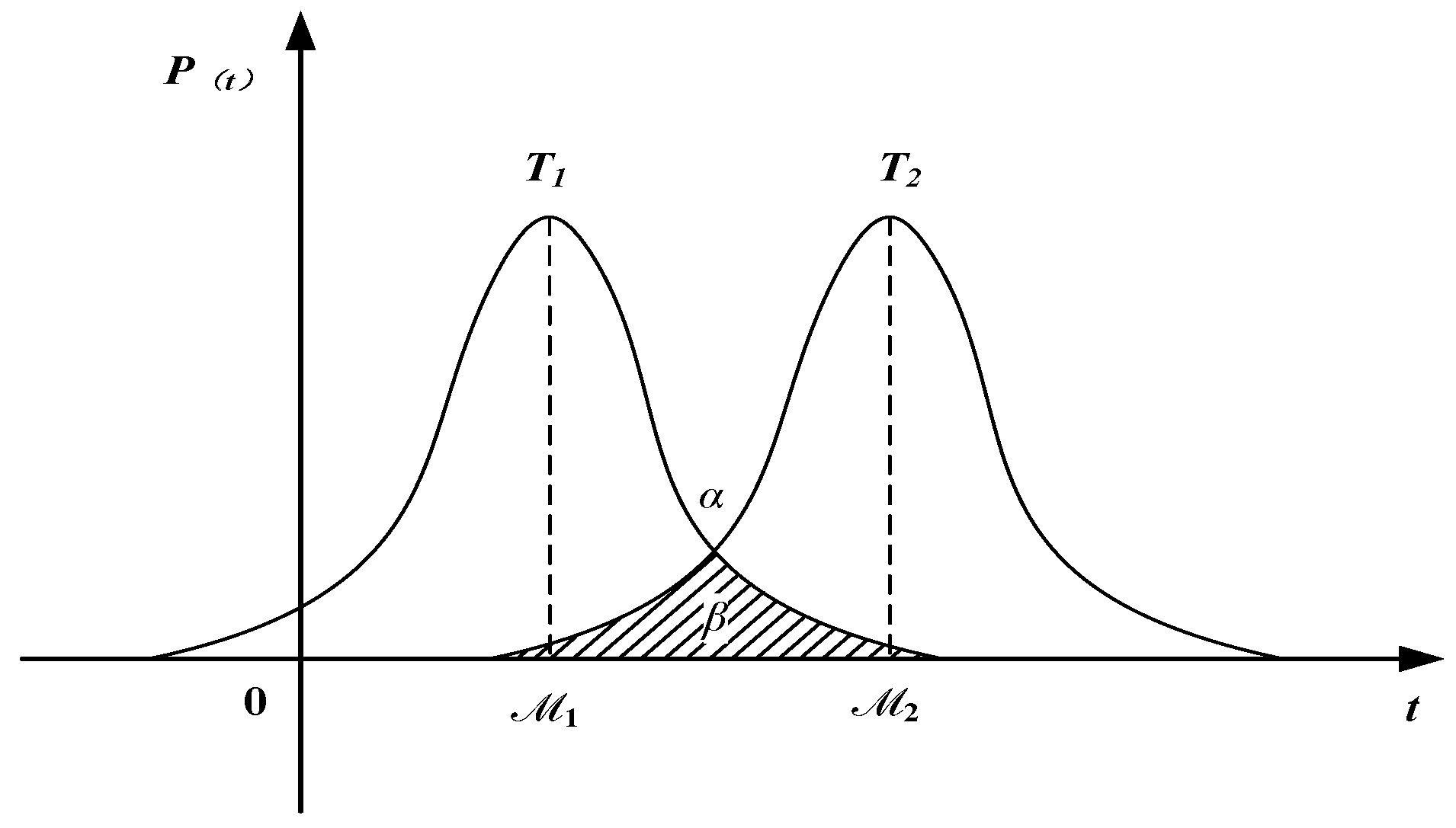
The random mixed-model disassembly operation time is an approximate normal distribution, [26]. The values of and determine the maximum disassembly operation time of the disassembly line, and thereby determine the disassembly operation beat of the disassembly operation line. As shown in Figure 1, the actual operation time of two stations can be considered as a normal distribution ().
As shown in Figure 1, the probability of the sum of disassembly operation time at station 1 greater than station 2 is , that is, the probability of the sum of disassembly operation time at station 1 setting as the disassembly operation beat of the entire production line. The size of can be determined by the area of the shadow: . In order to determine the disassembly operation beat between more stations, comparing all stations in pairs is adopted, and the maximum beat is reserved to participate in the next round until the disassembly beat is determined.
In the case of mixed-model disassembly, it is assumed that the disassembly operation time of the n-th disassembly task of the m-th product obeys a normal distribution with a mean of and a variance of (). The sum of the time of disassembly of the k-th workstation should be less than or equal to the disassembly operation beat (i.e. ) [26]:
The disassembly complexity of mixed-model disassembly line is directly affected by the degree of difference between products. Considering the various disturbance factors in the actual operation, the disassembly efficiency α is introduced to deal with the randomness, so as to obtain the disassembly beat of the disassembly line [26]. Set and specify , then:
Suppose the distribution function of the standard normal distribution is , then:
Detachable beats can be obtained as follow:
3. Balancing Model of Mixed-Model Disassembly Line in Random Working Environment
3.1. Mathematical Description
The disassembly line should not only consider the overall load balance of the disassembly production line, but also consider the differences in product structure, the constraint relationship between disassembly tasks, disassembly operation beat, disassembly cost and priority to disassemble the parts with high demand and high residual value.
Suppose there are a total of M types of decommissioned products in large quantities, and the product structure is similar. Set the number of workstations in disassembly line of mixed-model as K, and each time work with the minimum proportion unit (the proportion of product quantity divided by the maximum common divisor). Each unit has a total of N different tasks, and the part number on the disassembly line corresponds to the disassembly task in the set H. The disassembly task set is , and the tasks in the H are all divided into K workstations, that is, , where the task subset in the k-th disassembly station is , and each task must be assigned to the workstation; the matrix represents the priority constraint relationship of the disassembly task. If the i-th disassembly task takes precedence over the j-th disassembly task , then , otherwise ; companies engaged in dismantling services often sort the disassembly of parts of decommissioned products according to the demand for parts and components in the market, and preferentially dismantle parts with high market demand and high residual value, and indicates whether there is market demand for the n-th part of the m-th product. In the company’s disassembly work, it is necessary to consider the market demand, but also to reduce the cost of invalid disassembly operations. - cost of disassembly operation per unit time.
3.2. Modeling Assumption
To keep the model from getting too complicated, we made the following assumptions:
(1) In the mixed-model disassembly, the disassembly object takes products with similar structure and without modification.
(2) The sum of the time required for the disassembly work of each station cannot be greater than the disassembly line beat.
(3) Taking the classic linear disassembly production line as the research object, they are placed at a certain proportion and the smallest proportion unit is selected for research when multiple products are disassembled.
(4) All parts of the decommissioned products are completely disassembled, and similar disassembly tasks are assigned to the same workstation for disassembly, and each disassembly task does not interfere with each other.
(5) The task unit in the disassembly task set is inseparable, and one disassembly task can only correspond to one disassembly workstation.
(6) The constraint relationship between the various parts of the decommissioned product only has priority constraints, and the disassembly operation is performed in order of priority.
3.3. Model Development
The balance optimization problem of the disassembly operation line was considered from the following aspects:
(1) Minimum disassembly work stations. The number of disassembly line-opening workstations determines the cost of disassembly operation. Generally, the smaller the number of disassembly workstations, the lower the operating cost, while meeting the disassembly conditions. Therefore, it is required to minimize the number of disassembly work stations. The objective function is as follows:
(2) Load balancing index. It is necessary to ensure the load balancing of the disassembly line, as well as to improve the working efficiency as much as possible and reduce the idle rate of the workstation on the disassembly line. The objective function is as follows:
By combining Equations (2) and (7), the objective function can be transformed into:
(3) Priority to remove high-demand parts. When other conditions are the same, in order to ensure the efficiency of the enterprise, the parts with high market demand and high residual value should be disassembled as soon as possible. The objective function is as follows:
(4) Cost minimization of invalid operations. Disassembly enterprises should take into account the interests of enterprises on the basis of meeting market demands. Therefore, the cost of invalid disassembly should be minimized when establishing the disassembly line, and the idle time of each station should be minimized on the basis of load balancing. Then, the operating cost of the disassembly line can be determined based on the actual working time. The objective function is as follows:
When considering the line load balancing, it is possible to find the number of disassembly stations that meet the minimum load balance index [15]. Therefore, the objective function is mainly considered when establishing the integrated model.
Therefore, the multi-objective function of the mixed-model dismantling line is:
Constraints:
Equation (12) indicates that any one of the disassembly tasks n must be assigned to a disassembly workstation k, and cannot be subdivided; Equation (13) represents that the disassembly time of any one disassembly station cannot exceed the production tact of the disassembly line; Equation (14) shows that there is a sequence between the disassembly tasks, and the priority constraints cannot be violated; Equation (15) indicates the value interval of the disassembly workstation; Equation (16) means that all disassembly tasks must be assigned to the disassembly workstation and cannot be omitted; Equation (17) represents the number of disassembly tasks contained in any one of the workstations k.
4. Solution Algorithm
Simulated annealing algorithm (SA) and genetic algorithm (GA) have been widely used in combination optimization and have achieved good results [27]. In this paper, the characteristics of the balance problem of the mixed-model disassembly line, combined with the advantages of SA and GA, are solved by the adaptive simulated annealing genetic algorithm (ASAGA).
4.1. The Construction of Feasible Solutions
Disassembly tasks are randomly selected to ensure the diversity of the initial feasible solutions. In order to briefly explain the construction process of the feasible solutions, two types of decommissioned products A and B, are taken as examples to illustration. As shown in Figure 2(a),(b), disassembly tasks are only successively related without considering other constraints [28]. After the mixed-model integration, a new disassembly task sequence is obtained, as shown in Figure 2(c).
The numbers in the figure represent only the corresponding disassembly tasks. A straight line with an arrow indicates the priority relationship between the two disassembly tasks, such as ![Sustainability 11 02304 i001]() , indicating that task 1 takes precedence over task 2. If the disassembly task takes precedence over the disassembly task , then (,) = 1, otherwise, () = 0. The structural similarity coefficient of the two products A and B is . The priority matrix R is constructed according to the priority order between tasks:
, indicating that task 1 takes precedence over task 2. If the disassembly task takes precedence over the disassembly task , then (,) = 1, otherwise, () = 0. The structural similarity coefficient of the two products A and B is . The priority matrix R is constructed according to the priority order between tasks:
 , indicating that task 1 takes precedence over task 2. If the disassembly task takes precedence over the disassembly task , then (,) = 1, otherwise, () = 0. The structural similarity coefficient of the two products A and B is . The priority matrix R is constructed according to the priority order between tasks:
Feasible solution generation steps:
Step 1: The task that has not been assigned in R was randomly selected and there is no task allocated before the task or (that is, the elements of each column in the matrix R are all 0), and is taken as the disassembly task of current workstation K.
Step 2: Delete the task with the priority constraint relationship with the task , that is, remove the task before and after the task .
Step 3: Before all tasks are allocated, repeat the first two steps until all tasks are allocated, and the initial feasible solution can be obtained.
4.2. Adaptive Simulated Annealing Genetic Algorithm
SA can rapidly converge when solving the NP problem, but it is easy to fall into local optimization. Although GA has strong global optimization ability, it has insufficient local optimization ability when solving the NP problem. Therefore, in the basic genetic algorithm, the mutation operator and crossover operator are changed from the original fixed value to evolve with the change of algebra, which enables the algorithm to expand the search scope and enhance the global search ability in the early stage of optimization, and avoid the destruction of the optimal sequence and miss the optimal solution due to the high crossover and mutation probability in the later stage of the algorithm [29]. Moreover, the results obtained by GA are substituted into SA as the initial solution of SA, making full use of the advantages of GS and SA to make ASAGA have both the ability of rapid convergence, global search and getting rid of local optimal, so as to enhance the solving performance of the algorithm.
(1) Selection of encoding mode. In genetic algorithm, binary coding is mostly adopted. Considering that the multi-product and multi-task correspond to the workstation and there is priority relationship between the task and target, real coding is adopted to make the corresponding relationship between the task and workstation clearer.
(2) Select operation. Take the target function as the fitness function and select the probability . The greater the probability is, the easier the individual will be retained.
(3) Cross operation. The chromosomes in the parent generation are paired with each other, and two points in the sequence 1 and 2 are randomly selected for crossover. The sequence before the crossover point 1 remains unchanged, and the crossover point 2 is the same. The specific crossover operation is shown in Figure 3(a).
The intersection of parent and will form new individuals and . Considering that the algorithm should try to search in a wide range in the early stage and select a small crossover probability to avoid destroying the sequence of the optimal solution when it is close to the optimal value in the later stage, the traditional genetic crossover operator is improved into an adaptive crossover operator that evolves with the change of population algebra.
(4) Mutation operation. After the completion of (3), was used as the parent for single-point insertion mutation. The mutation point is randomly selected in the parent sequence, and the location where the mutation can be carried out should be in the middle of the adjacent tight before and after tasks. The specific mutation operation is shown in Figure 3(b). Ch-1 is obtained when keeping the priority relationship of tight before and after tasks unchanged, and randomly selecting a point in the mutational position to carry out the mutation. If the mutation operation cannot be completed due to the priority constraint relationship between tasks, then randomly finding a new insertion point to carry out the mutation operation. The selection method of mutation operator is similar to that of crossover operator. Adaptive mutation operator is adopted:
(5) Simulated annealing operation. The new population generated by GA is used as the input population of SA for annealing operation. The fitness value of the new population was calculated and compared with that of the parent population. According to the Metropolis criterion, if , it accepts the current individual and replaces the original old individual with that individual. Otherwise, it accepts the new individual instead of the old one with probability . In simulated annealing, the algorithm completes an optimization process for each cooling down, and the cooling times are the number of iterations. The cooling formula is as follows:
4.3. Algorithm Steps
Step 1: Initialize the population and parameters, set the population size = 100; Number of iterations = 100;,; , ; Initial temperature = 100; temperature drop coefficient = 0.95, , etc.
Step 2: Generate the initial population according to the priority matrix R.
Step 3: Encode and decode the initial population, take the target function as the fitness function, and record the fitness value of all individuals in the current population.
Step 4: After adaptive crossover and mutation, select elite individuals from all individuals.
Step 5: Perform simulated annealing, calculate and update the fitness value , and judge whether to receive the new solution according to the Metropolis criterion.
Step 6: If , execute cooling operation as , turn to step 4. Otherwise, find the optimal solution in the new population.
The whole flowchart of the ASAGA algorithm is shown in Figure 4.
5. Case Validation
To verify the effectiveness of the algorithm, MATLAB 2014a was used for programming. In order to ensure the best overall performance, the random operation time of the disassembly line, load balancing index, demand index of parts and the minimization of invalid activity cost were taken into account comprehensively, and the final objective function was obtained after the normalization of the optimization objective in Section 2.3. [30]:
In formula (21), , and respectively represent the value of the objective function corresponding to the disassembly of the parts of the n-th disassembly task in the disassembly production line; and are the maximum values of the target function; and are the minimum values of the target function; is the weight factor, , may be measured by the load of the removal line, the market demand for this part, and the cost of invalid removal operation.
Taking three kinds of decommissioned engines A, B and C as research objects, the number of disassembly tasks (N = 57) was obtained by mixing them in a ratio of 1:2:1 and composite processing. The explosion diagram and priority sequence of the mixed-model sequence are shown in Figure 5 and Figure 6.
The number in the upper left corner of the task number represents the disassembly time of the part. The average disassembly time obtained from the sample measurement by the stopwatch can be used to calculate the actual disassembly operation time according to formula (5). After field investigation, this paper takes 0.03 yuan as the comprehensive cost of disassembly operation per unit time (water, electricity, labor, site and equipment, etc.). In order to verify the effectiveness of the proposed algorithm and simulate the impact of random work environment on the disassembly operation, the computational results of three different are compared when other parameters were controlled constantly as shown in Table 1.
As shown in Table 1, with different disassembly efficiency , the optimization scheme proposed in this paper is superior to the other two algorithms. Further explanation is made with a value of = 0.95, and the solution results are shown in Table 2.
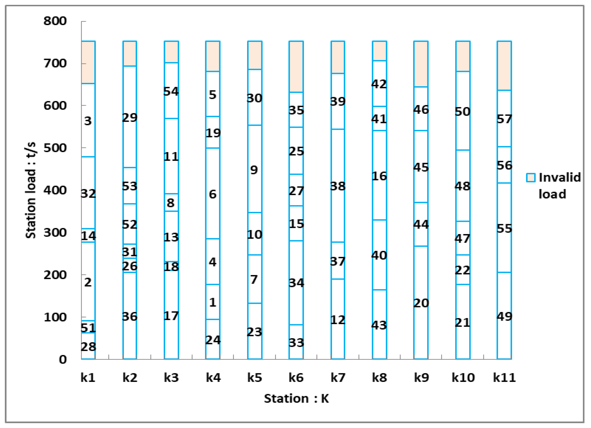
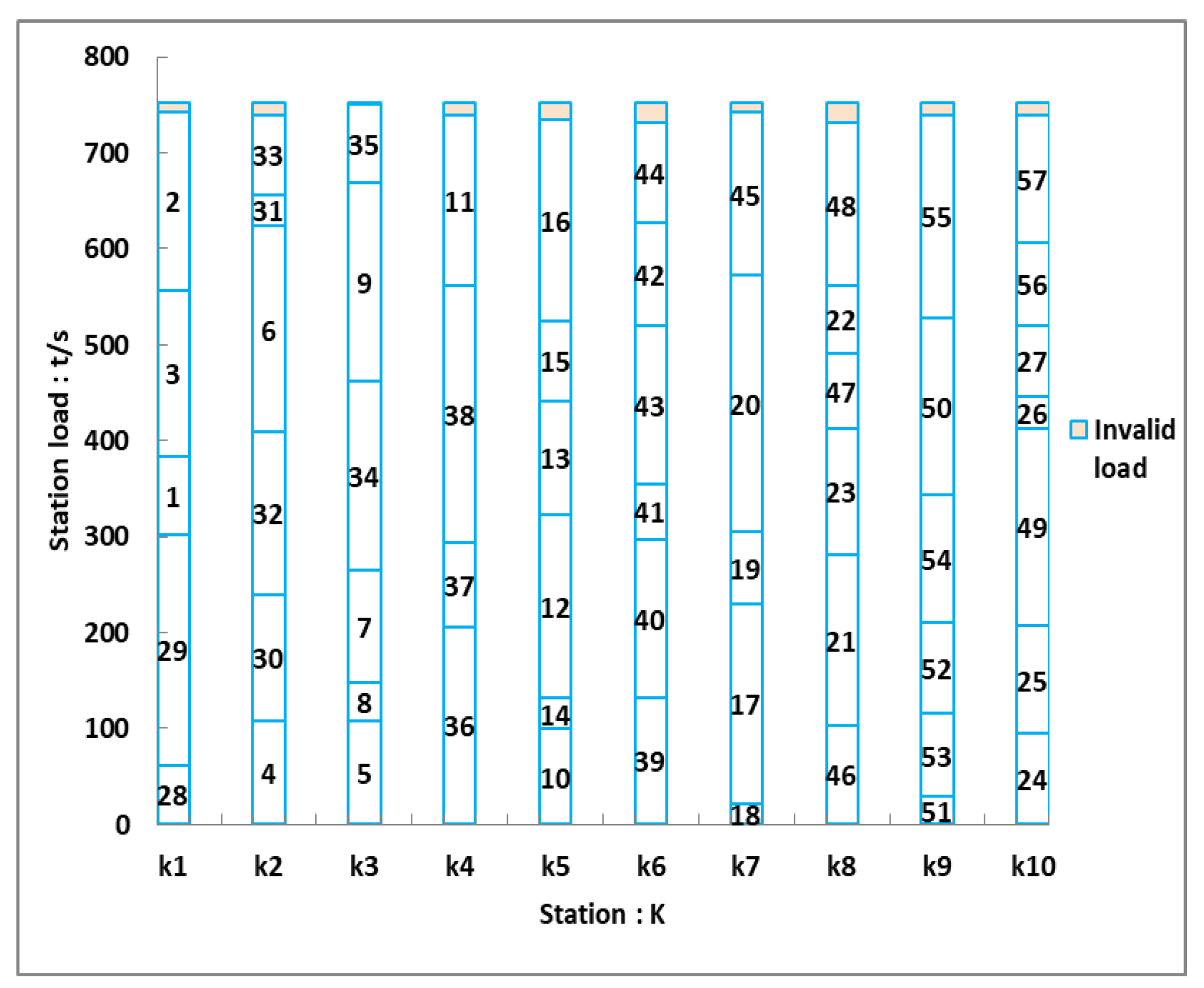
First, the minimum quantity of opening stations obtained by the ASAGA algorithm is one less than the minimum station quantity obtained by SA and GA in Table 2, which largely saves the disassembly operation cost. Second, the load balancing index and invalid activity cost of the disassembly line is used to measure whether the workstations selected in the disassembly line are running effectively and reasonably. According to the comparison results of the optimal disassembly scheme obtained by the three algorithms, the ASAGA algorithm has a good performance in terms of the load balancing index and invalid activity cost. From the perspective of preferential disassembly of parts with high demand and high residual value, the ASAGA algorithm does not seem to perform particularly well. The reason may be to make the load of the disassembly line more balanced and make the overall performance of the disassembly line more superior in the solving process of the algorithm, and the comparison of the comprehensive performance index (Fm) of the disassembly line in Table 2 proves this view. In conclusion, the ASAGA proposed in this paper is more advantageous than GA and SA, and the correctness of the model is verified simultaneously. The station load distributions of the optimal scheme obtained by each algorithm were shown in Figure 7, Figure 8 and Figure 9.
6. Conclusions
Aiming at the deficiency of traditional research on the disassembly line balance, a mixed-model disassembly model with the minimum number of stations, load balancing index, priority disassembly of parts in demand and the minimization of invalid activity cost was established by introducing structural similarity coefficient and taking the randomness of actual disassembly operation environment into consideration. An adaptive simulated annealing genetic algorithm was adopted to solve the model and an actual case was used to verify the proposed model and algorithm. The conclusions are as follows:
(1) Considering the various types of products in the actual disassembly process and the uncertainty of disassembly operation time, the product similarity coefficient was used to measure the multiple products. The disassembly efficiency was taken as the disturbance variable and the product category Pm was introduced into the model to establish the mixed-model disassembly line balance model in a random operating environment.
(2) According to the characteristics of mixed-model disassembly and combining the advantages of GA and SA, an adaptive simulated annealing genetic algorithm was proposed. The adaptive operator improved the convergence speed of the algorithm, and it was not easy to destroy the optimal solution sequence in the later stage of the algorithm. The results obtained by genetic algorithm can be used as the initial solution of simulated annealing operation, so that the algorithm has both local and global search capabilities.
(3) In this paper, the mixed-model disassembly of engine products with 57 disassembly tasks was verified by simulating the random operating environment and setting different disassembly. The results indicated that the proposed algorithm used in the smallest number, load balance index, invalid operation costs and disassembly line overall performance was superior to contrast groups, and the correctness and validity of the model were verified.
Based on the actual disassembly operation, this paper provides a new solution to the disassembly line balance problem of the mixed-model in a random operation environment, which has an important guiding significance for energy saving and consumption reduction and an efficient operation of disassembly link in the reverse supply chain. However, the influence of the structure complexity of decommissioned products on the disassembly operation and the disassembly mode are not considered, and we will do further research in the future.
Author Contributions
W.L. performed the experiments and wrote the paper; X.X. is the project leader; Z.Z. conceived and designed the models; W.L. analyzed the data; J.C. and X.L. contributed reagents/materials/analysis tools.
Funding
This research was funded by the National Natural Science Foundation of China (grant number 51805385, 51604196), the Natural Science Foundation of Hubei Province (grant number 2018CFB265), Fund of State Key Laboratory of Mineral Processing (grant number BGRIMM-KJSKL-2016-06), and China Postdoctoral Science Foundation (grant number 2017M612522).
Acknowledgments
Thanks for all the authors of the references who give us inspiration and help. The authors are grateful to the editors and anonymous reviewers for their valuable comments that improved the quality of this paper.
Conflicts of Interest
The authors declare no conflicts of interest.
References
- Idiano, D.; Rosa, P. Remanufacturing in industry: Advices from the field. Int. J. Adv. Manuf. Technol. 2016, 86, 2575–2584. [Google Scholar]
- Tao, F.; Cheng, Y.; Zhang, L.; Nee, A.Y.C. Advanced manufacturing systems: Socialization characteristics and trends. J. Intell. Manuf. 2017, 28, 1079–1094. [Google Scholar] [CrossRef]
- Kwak, M.J. Optimal Line Design of New and Remanufactured Products: A Model for Maximum Profit and Market Share with Environmental Consideration. Sustainability 2018, 10, 4283. [Google Scholar] [CrossRef]
- Wang, L.H.; Wang, X.V.; Gao, L.; Va’ncza, J. A cloud-based approach for WEEE remanufacturing. Cirp Ann. Manuf. Technol. 2014, 63, 409–412. [Google Scholar] [CrossRef] [Green Version]
- Wang, Q.; Tang, D.B.; Li, S.P.; Yang, J.; Salido, M.A.; Giret, A.; Zhu, H.H. An Optimization Approach for the Coordinated Low-Carbon Design of Product Family and Remanufactured Products. Sustainability 2019, 11, 460. [Google Scholar] [CrossRef]
- Ilgin, M.A.; Akçay, H.; Araz, C. Disassembly line balancing using linear physical programming. Int. J. Prod. Res. 2017, 55, 6108–6119. [Google Scholar] [CrossRef]
- Priyono, A.; Ijomah, W.; Bititci, U. Disassembly for remanufacturing: A systematic literature review, new model development and future research needs. J. Ind. Eng. Manag. 2016, 9, 899–932. [Google Scholar] [CrossRef]
- Hu, B.T.; Feng, Y.X.; Zheng, H.; Tan, J.R. Sequence Planning for Selective Disassembly Aiming at Reducing Energy Consumption Using a Constraints Relation Graph and Improved Ant Colony Optimization Algorithm. Energies 2018, 11, 2106. [Google Scholar] [CrossRef]
- Süleyman, M.; Zeynel, A.; Kürşad, A.; Eren, Ö.; Alexandre, D. A solution approach based on beam search algorithm for disassembly line balancing problem. J. Manuf. Syst. 2016, 41, 188–200. [Google Scholar]
- Shaaban, S.; Kalayci, C.B.; Gupta, S.M. Ant colony optimization for sequence-dependent disassembly line balancing problem. J. Manuf. Technol. Manag. 2013, 24, 413–427. [Google Scholar]
- Gungor, A.; Gupta, S.M. A solution approach to the disassembly line balancing problem in the presence of task failures. Int. J. Prod. Res. 2001, 39, 1427–1467. [Google Scholar] [CrossRef]
- McGovern, S.M.; Gupta, S.M. A balancing method and genetic algorithm for disassembly line balancing. Eur. J. Oper. Res. 2007, 179, 692–708. [Google Scholar] [CrossRef]
- Ding, L.P.; Feng, Y.X.; Tan, J.R.; Gao, Y.C. A new multi-objective ant colony algorithm for solving the disassembly line balancing problem. Int. J. Adv. Manuf. Technol. 2010, 48, 761–771. [Google Scholar] [CrossRef]
- Lu, C.; Liu, Y.C. A disassembly sequence planning approach with an advanced immune algorithm. Proc. Inst. Mech. Eng. 2012, 226, 2739–2749. [Google Scholar] [CrossRef]
- Kalayci, C.B.; Polat, O.; Gupta, S.M. A variable neighbourhood search algorithm for disassembly lines. J. Manuf. Technol. Manag. 2015, 26, 182–194. [Google Scholar] [CrossRef]
- Alshibli, M.; ElSayed, A.; Kongar, E.; Sobh, T.; Gupta, S.M. Disassembly Sequencing Using Tabu Search. J. Intell. Robot. Syst. 2016, 82, 69–79. [Google Scholar] [CrossRef]
- Alshibli, M.; EISayed, A.; Kongar, E.; Sobh, T.; Gupta, S.M. A Robust Robotic Disassembly Sequence Design Using Orthogonal Arrays and Task Allocation. Robotics 2019, 8, 20. [Google Scholar] [CrossRef]
- Kalayci, C.B.; Gupta, S.M. A particle swarm optimization algorithm with neighborhood-based mutation for sequence-dependent disassembly line balancing problem. Int. J. Adv. Manuf. Technol. 2013, 69, 197–209. [Google Scholar] [CrossRef]
- Liu, J.; Wang, S.W. Balancing disassembly line in product recovery to promote the coordinated development of economy and environment. Sustainability 2017, 9, 309. [Google Scholar] [CrossRef]
- Kalayci, C.B.; Polat, O.; Gupta, S.M. A hybrid genetic algorithm for sequence-dependent disassembly line balancing problem. Ann. Oper. Res. 2016, 242, 321–354. [Google Scholar] [CrossRef]
- Gao, Y.C.; Wang, Q.R.; Feng, Y.X.; Zheng, H.; Zheng, B.; Tan, J.R. An Energy-Saving Optimization Method of Dynamic Scheduling for Disassembly Line. Energies 2018, 11, 1261. [Google Scholar] [CrossRef]
- Guiras, Z.H.; Turki, S.; Rezg, N.; Dolgui, A. Optimization of Two-Level Disassembly/Remanufacturing/Assembly System with an Integrated Maintenance Strategy. Appl. Sci. 2018, 8, 666. [Google Scholar] [CrossRef]
- Liu, J.Y.; Zhou, Z.D.; Pham, D.T.; Xu, W.J.; Yan, J.W.; Liu, A.M.; Ji, C.Q.; Liu, Q. An improved multi-objective discrete bees algorithm for robotic disassembly line balancing problem in remanufacturing. Int. J. Adv. Manuf. Technol. 2018, 97, 3937–3962. [Google Scholar] [CrossRef]
- Kalayci, C.B.; Hancilar, A.; Gungor, A.; Gupta, S.M. Multi-objective fuzzy disassembly line balancing using a hybrid discrete artificial bee colony algorithm. J. Manuf. Syst. 2015, 37, 672–682. [Google Scholar] [CrossRef] [Green Version]
- Kim, H.W.; Lee, D.H. A sample average approximation algorithm for selective disassembly sequencing with abnormal disassembly operations and random operation times. Int. J. Adv. Manuf. Technol. 2018, 96, 1341–1354. [Google Scholar] [CrossRef]
- Bentaha, M.L.; Olga, B.; Dolgui, A. An exact solution approach for disassembly line balancing problem under uncertainty of the task processing times. Int. J. Prod. Res. 2015, 53, 1807–1818. [Google Scholar] [CrossRef]
- Kalayci, C.B.; Gupta, S.M. Simulated Annealing Algorithm for Solving Sequence-Dependent Disassembly Line Balancing Problem. IFAC Proc. Vol. 2013, 46, 93–98. [Google Scholar] [CrossRef]
- Chutima, P.; Chimklai, P. Multi-objective two-sided mixed-model assembly line balancing using particle swarm optimisation with negative knowledge. Comput. Ind. Eng. 2012, 62, 39–55. [Google Scholar] [CrossRef]
- Wang, Y.; Li, K.L.; Li, K.Q. Dynamic Data Allocation and Task Scheduling on Multiprocessor Systems with NVM-Based SPM. IEEE Access 2019, 7, 1548–1559. [Google Scholar] [CrossRef]
- Kalayci, C.B.; Gupta, S.M. A hybrid genetic algorithm approach for disassembly line balancing. In Proceedings of the 42nd Annual Meeting of Decision Science Institute, Boston, MA, USA, 19–22 November 2011; pp. 2142–2148. [Google Scholar]
Figure 1.
Normal distribution of disassembly work time of two stations.

Figure 2.
(a) Disassembly sequence of product A; (b) disassembly sequence of product B; (c) disassembly sequence of mixed products of A and B.
Figure 2.
(a) Disassembly sequence of product A; (b) disassembly sequence of product B; (c) disassembly sequence of mixed products of A and B.

Figure 3.
(a) Cross operation diagram; (b) mutation operation diagram.

Figure 4.
Flowchart of the ASAGA algorithm.

Figure 5.
Schematic diagram of engine parts.

Figure 6.
The priority diagram of equipment parts.

Figure 7.
GA station load distribution map.

Figure 8.
SA station load distribution map.

Figure 9.
ASAGA station load distribution map.


Table 1.
Comparison of disassembly schemes with different disassembly efficiency .
| Algorithm | Number of stations | Load balancing index | Invalid operating cost/yuan | ||
|---|---|---|---|---|---|
| 0.90 | 752 | GA | 11 | 77792.98 | 26.48 |
| SA | 11 | 80247.03 | 26.48 | ||
| ASAGA | 10 | 2044.20 | 3.92 | ||
| 0.95 | 758 | GA | 11 | 78082.15 | 26.51 |
| SA | 11 | 80579.55 | 26.51 | ||
| ASAGA | 10 | 1923.02 | 3.77 | ||
| 0.99 | 770.4 | GA | 11 | 80549.86 | 26.92 |
| SA | 11 | 83130.09 | 26.92 | ||
| ASAGA | 10 | 1969.49 | 3.81 |
Table 2.
Comparison of optimal allocation schemes for GA, PSO and ASAGA algorithms.
| Algorithm | StationF1 | Task number | Payload (s) | Invalid load (s) | F2 | F3 | F4 | Fm |
|---|---|---|---|---|---|---|---|---|
| GA | 1 | 28,51,2,14,32,3 | 657.99 | 100.01 | 10001.80 | 40.00 | 3.00 | 0.460 |
| 2 | 36,26,31,52,53,29 | 699.64 | 58.36 | 3406.36 | 68.00 | 1.75 | ||
| 3 | 17,18,13,8,11,54 | 707.97 | 50.04 | 2503.50 | 40.00 | 1.50 | ||
| 4 | 24,1,4,6,19,5 | 687.14 | 70.86 | 5020.79 | 76.00 | 2.13 | ||
| 5 | 23,7,10,9,30 | 691.31 | 66.69 | 4447.96 | 24.00 | 2.00 | ||
| 6 | 33,34,15,27,25,35 | 637.17 | 120.83 | 14600.25 | 28.00 | 3.62 | ||
| 7 | 12,37,38,39 | 682.98 | 75.02 | 5628.30 | 20.00 | 2.25 | ||
| 8 | 43,40,16,41,42 | 712.13 | 45.87 | 2104.10 | 48.00 | 1.38 | ||
| 9 | 20,44,45,46 | 649.66 | 108.34 | 11737.12 | 48.00 | 3.25 | ||
| 10 | 21,22,47,48,50 | 687.14 | 70.86 | 5020.79 | 28.00 | 2.13 | ||
| 11 | 49,55,56,57 | 641.33 | 116.67 | 13611.19 | 28.00 | 3.50 | ||
| SA | 1 | 36,1,2,10,32 | 749.61 | 8.39 | 70.39 | 20.00 | 0.25 | 0.703 |
| 2 | 28,8,3,51,17,26,13 | 674.65 | 83.35 | 6947.39 | 64.00 | 2.50 | ||
| 3 | 52,14,18,15,53,31,54,11 | 666.32 | 91.68 | 8405.22 | 68.00 | 2.75 | ||
| 4 | 29,19,23,30,33, | 666.32 | 91.68 | 8405.22 | 48.00 | 2.75 | ||
| 5 | 24,27,34,25,37,4 | 678.81 | 79.19 | 6270.50 | 40.00 | 2.38 | ||
| 6 | 5,6,7,9 | 649.66 | 108.34 | 11737.12 | 36.00 | 3.25 | ||
| 7 | 12,35,38,39 | 678.81 | 79.19 | 6270.50 | 20.00 | 2.38 | ||
| 8 | 16,40,20 | 649.66 | 108.34 | 11737.12 | 40.00 | 3.25 | ||
| 9 | 43,41,42,44,21,22 | 687.14 | 70.86 | 5020.79 | 48.00 | 2.13 | ||
| 10 | 45,46,47,48,50 | 712.13 | 45.87 | 2104.10 | 36.00 | 1.38 | ||
| 11 | 55,49,56,57 | 641.33 | 116.67 | 13611.19 | 28.00 | 3.50 | ||
| ASAGA | 1 | 28,29,1,3,2 | 749.61 | 8.39 | 70.39 | 36.00 | 0.25 | 0.455 |
| 2 | 4,30,32,6,31,33 | 745.45 | 12.55 | 157.62 | 40.00 | 0.38 | ||
| 3 | 5,8,7,34,9,35 | 757.94 | 0.06 | 0.00 | 44.00 | 0.00 | ||
| 4 | 36,37,38,11 | 745.45 | 12.55 | 157.62 | 32.00 | 0.38 | ||
| 5 | 10,14,12,13,15,16 | 741.28 | 16.72 | 279.52 | 28.00 | 0.50 | ||
| 6 | 39,40,41,43,42,44 | 737.12 | 20.88 | 436.12 | 52.00 | 0.63 | ||
| 7 | 18,17,19,20,45 | 749.61 | 8.39 | 70.39 | 68.00 | 0.25 | ||
| 8 | 46,21,23,47,22,48 | 737.12 | 20.88 | 436.12 | 40.00 | 0.63 | ||
| 9 | 51,53,52,54,50,55 | 745.45 | 12.55 | 157.62 | 36.00 | 0.38 | ||
| 10 | 24,25,49,26,27,56,57 | 745.45 | 12.55 | 157.62 | 72.00 | 0.38 |
Remarks: The demand indexes of 1–57 parts are 1, 1, 3, 1, 4, 2, 1, 1, 2, 1, 4, 1, 1, 2, 1, 1, 1, 2, 7, 6, 1, 2, 1, 4, 1, 7, 1, 2, 2, 1, 4, 1, 1, 1, 2, 1, 2, 1, 1, 3, 1, 5, 2, 1, 1, 4, 1, 1, 2, 2, 1, 1, 2, 1, 2, 2, 1.
© 2019 by the authors. Licensee MDPI, Basel, Switzerland. This article is an open access article distributed under the terms and conditions of the Creative Commons Attribution (CC BY) license (http://creativecommons.org/licenses/by/4.0/).
Share and Cite
MDPI and ACS Style
Xia, X.; Liu, W.; Zhang, Z.; Wang, L.; Cao, J.; Liu, X. A Balancing Method of Mixed-model Disassembly Line in Random Working Environment. Sustainability 2019, 11, 2304. https://doi.org/10.3390/su11082304
AMA Style
Xia X, Liu W, Zhang Z, Wang L, Cao J, Liu X. A Balancing Method of Mixed-model Disassembly Line in Random Working Environment. Sustainability. 2019; 11(8):2304. https://doi.org/10.3390/su11082304
Chicago/Turabian StyleXia, Xuhui, Wei Liu, Zelin Zhang, Lei Wang, Jianhua Cao, and Xiang Liu. 2019. "A Balancing Method of Mixed-model Disassembly Line in Random Working Environment" Sustainability 11, no. 8: 2304. https://doi.org/10.3390/su11082304
Note that from the first issue of 2016, this journal uses article numbers instead of page numbers. See further details here.