Dynamic Scheduling Based on Predicted Inventory Variation Rate for Public Bicycle System


Abstract
1. Introduction
2. Properties of a Station
2.1. Inventory Variation Rate
2.2. Predicted Inventory Rate
2.3. Rebalancing Demand
2.4. Latest Arrival Time
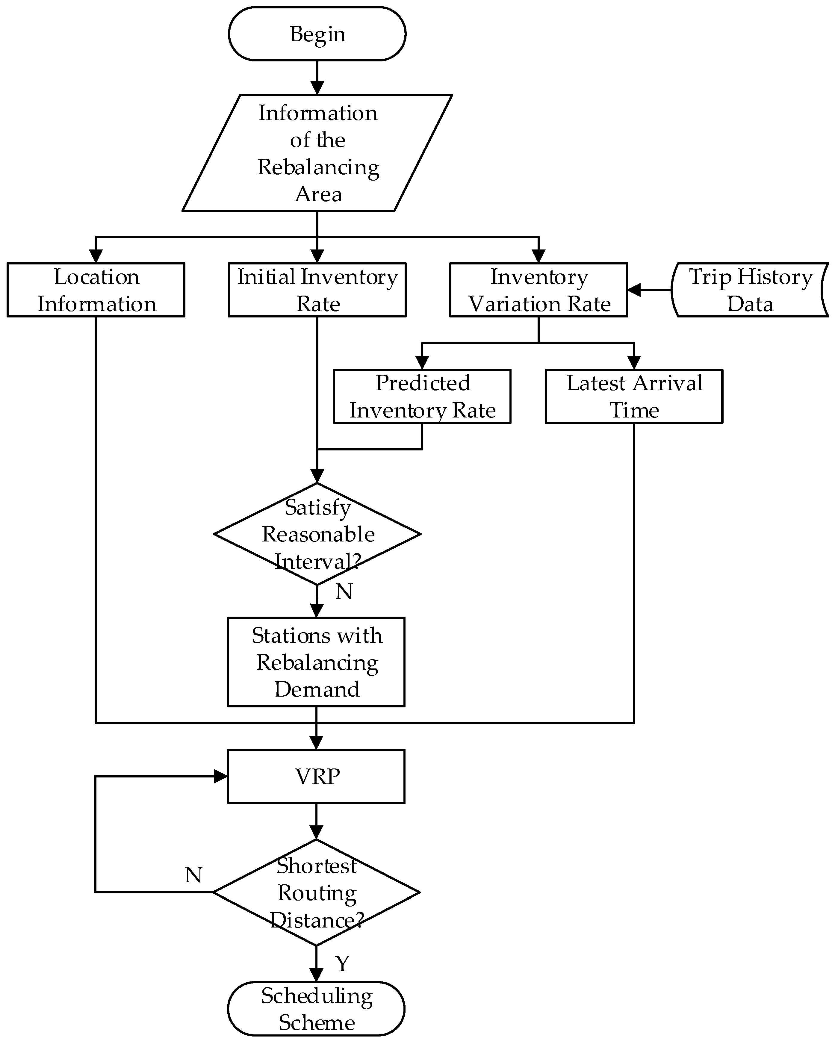
3. Methodology
Scheduling Scheme
4. Validation of DS-PIVR
5. Discussion
6. Conclusions
Author Contributions
Funding
Acknowledgments
Conflicts of Interest
References
- Martin, E.; Cohen, A.; Botha, J.; Shaheen, S. Bikesharing and Bicycle Safety. Mineta Transportation Institute Publications. Available online: http://transweb.sjsu.edu/research/bikesharing-and-bicycle-safety (accessed on 18 March 2019).
- Shaheen, S.; Martin, E.; Cohen, A. Public Bikesharing and Modal Shift Behavior: A Comparative Study of Early Bikesharing Systems in North America. Int. J. Transp. 2013, 1, 35–54. [Google Scholar] [CrossRef]
- Pucher, J.; Buehler, R. Cycling towards a more sustainable transport future. Transp. Rev. 2017, 37, 689–694. [Google Scholar] [CrossRef]
- Fishman, E. Bikeshare: A Review of Recent Literature. Transp. Rev. 2016, 36, 92–113. [Google Scholar] [CrossRef]
- Lu, T.; Mondschein, A.; Buehler, R.; Hankey, S. Adding temporal information to direct-demand models: Hourly estimation of bicycle and pedestrian traffic in Blacksburg, VA. Transp. Res. Part D 2018, 63, 244–260. [Google Scholar] [CrossRef]
- Faghih-Imani, A.; Hampshire, R.; Marla, L.; Eluru, N. An empirical analysis of bike sharing usage and rebalancing: Evidence from Barcelona and Seville. Transp. Res. Part A 2017, 97, 177–191. [Google Scholar] [CrossRef]
- Wergin, J.; Buehler, R. Where Do Bikeshare Bikes Actually Go? Analysis of Capital Bikeshare Trips with GPS Data. Transp. Res. Rec. 2017, 2662, 12–21. [Google Scholar] [CrossRef]
- Hankey, S.; Lu, T.; Mondschein, A.; Buehler, R. Spatial models of active travel in small communities: Merging the goals of traffic monitoring and direct-demand modeling. J. Transp. Health Part B 2017, 7, 149–159. [Google Scholar] [CrossRef]
- Lu, T.; Buehler, R.; Mondschein, A.; Hankey, S. Designing a Bicycle and Pedestrian Traffic Monitoring Program to Estimate Annual Average Daily Traffic in a Small Rural College Town. Transp. Res. Part D 2017, 53, 193–204. [Google Scholar] [CrossRef]
- Shaheen, S.; Guzman, S.; Zhang, H. Bikesharing in Europe, the Americas, and Asia: Past, Present, and Future. Transp. Res. Rec. 2011, 2143, 159–167. [Google Scholar] [CrossRef]
- Cagliero, L.; Cerquitelli, T.; Chiusano, S.; Garza, P.; Ricupero, G.; Baralis, E. Characterizing Situations of Dock Overload in Bicycle Sharing Stations. Appl. Sci. 2018, 8, 2521. [Google Scholar] [CrossRef]
- Li, L.; Shan, M. Bidirectional Incentive Model for Bicycle Redistribution of a Bicycle Sharing System during Rush Hour. Sustainability 2016, 8, 1299. [Google Scholar] [CrossRef]
- Zhou, Y.; Wang, L.; Zhong, R.; Tan, Y. A Markov Chain Based Demand Prediction Model for Stations in Bike Sharing Systems. Math. Prob. Eng. 2016, 2016, 8028714. [Google Scholar] [CrossRef]
- Raviv, T.; Kolka, O. Optimal Inventory Management of a Bike-sharing Station. IIE Trans. 2013, 45, 1077–1093. [Google Scholar] [CrossRef]
- Xu, C.; Ji, J.; Liu, P. The Station-free Sharing Bike Demand forecasting with a Deep Learning Approach and Large-scale Datasets. Transp. Res. Part C 2018, 95, 47–60. [Google Scholar] [CrossRef]
- Feng, Y.; Wang, S. A Forecast for Bicycle Rental Demand based on Random Forests and Multiple Linear Regression. In Proceedings of the IEEE/ACIS International Conference on Computer and Information Science, Wuhan, China, 24–26 May 2017. [Google Scholar] [CrossRef]
- Ashqar, H.I.; Elhenawy, M.; Almannaa, M.H.; Ghanem, A.; Rakha, H.A.; House, L. Modeling Bike Availability in a Bike-Sharing System Using Machine Learning. In Proceedings of the 5th IEEE International Conference on Models and Technologies for Intelligent Transportation Systems, Naples, Italy, 26–28 June 2017. [Google Scholar] [CrossRef]
- Jiang, J.; Lin, F.; Fan, J.; Lv, H.; Wu, J. A Destination Prediction Network Based on Spatiotemporal Data for Bike-Sharing. Complexity 2019, 2019, 7643905. [Google Scholar] [CrossRef]
- Dong, H.; Shi, C.; Chen, N.; Liu, D. Clustering Division of Public Bicycle Scheduling Regional Based on Association Rules. Bullet. Sci. Techn. 2013, 29, 209–212. (In Chinese) [Google Scholar] [CrossRef]
- Almannaa, M.H.; Elhenawy, M.; Ghanem, A.; Ashqar, H.I.; Rakha, H.A. Network-Wide Bike Availability Clustering Using the College Admission Algorithm: A Case Study of San Francisco Bay Area. In Proceedings of the 5th IEEE International Conference on Models and Technologies for Intelligent Transportation Systems, Naples, Italy, 26–28 June 2017. [Google Scholar] [CrossRef]
- Forma, I.A.; Raviv, T.; Tzur, M. A 3-step Math Heuristic for the Static Repositioning Problem in Bike-sharing Systems. Transp. Res. Part B 2015, 71, 230–247. [Google Scholar] [CrossRef]
- Dell’Amico, M.; Hadjicostantinou, E.; Iori, M.; Novellani, S. The Bike Sharing Rebalancing Problem: Mathematical Formulations and Benchmark Instances. Omega 2014, 45, 7–19. [Google Scholar] [CrossRef]
- Erdogan, G.; Battarra, M.; Calvo, R.W. An Exact Algorithm for the Static Rebalancing Problem arising in Bicycle Sharing Systems. Eur. J. Oper. Res. 2015, 245, 667–679. [Google Scholar] [CrossRef]
- Li, Y.; Szeto, W.Y.; Long, J.; Shui, C.S. A Multiple Type Bike Repositioning Problem. Transp. Res Part B 2016, 90, 263–278. [Google Scholar] [CrossRef]
- Szeto, W.; Liu, Y.; Ho, S. Chemical Reaction Optimization for Solving a Static Bike Repositioning Problem. Transp. Res. Part D 2016, 47, 104–135. [Google Scholar] [CrossRef]
- Braekers, K.; Ramaekers, K.; Nieuwenhuyse, I.V. The Vehicle Routing Problem: State of the Art Classification and Review. Comput. Ind. Eng. 2016, 99, 300–313. [Google Scholar] [CrossRef]
- Raviv, T.; Tzur, M.; Forma, I.A. Static Repositioning in a Bike-sharing System: Models and Solution Approaches. Eur. J. Transp. Logist. 2013, 2, 187–229. [Google Scholar] [CrossRef]
- Schuijbroek, J.; Hampshire, R.C.; Hoeve, W.J. Inventory Rebalancing and Vehicle Routing in Bike Sharing Systems. Eur. J. Oper. Res. 2017, 257, 992–1004. [Google Scholar] [CrossRef]
- Shui, C.S.; Szeto, W.Y. Dynamic Green Bike Repositioning Problem—A Hybrid Rolling Horizon Artificial Bee Colony Algorithm Approach. Transp. Res. Part D 2018, 60, 119–136. [Google Scholar] [CrossRef]
- Zhang, D.; Yu, C.; Desai, J.; Lau, H.Y.K.; Srivathsan, S. A Time-space Network Flow Approach to Dynamic Repositioning in Bicycle Sharing Systems. Transp. Res. Part B 2017, 103, 188–207. [Google Scholar] [CrossRef]
- Yu, K.; Yang, J. MILP Model and a Rolling Horizon Algorithm for Crane Scheduling in a Hybrid Storage Container Terminal. Math. Prob. Eng. 2019, 2019, 4739376. [Google Scholar] [CrossRef]
- Gagniuc, P.A. Markov Chains: From Theory to Implementation and Experimentation; John Wiley & Sons: Hoboken, NJ, USA, 2017. [Google Scholar]
- Miller, C.E.; Tucker, A.W.; Zemlin, R.A. Integer Programming Formulation of Traveling Salesman Problems. J. ACM 1960, 7, 326–329. [Google Scholar] [CrossRef]
- Gillet, B.; Miller, L. A Heuristic Algorithm for the Vehicle-Dispatch Problem. Oper. Res. 1974, 22, 340–349. [Google Scholar] [CrossRef]
- Perboli, G.; Rosano, M.; Saint-Guillain, M.; Rizzo, P. Simulation-optimisation framework for City Logistics: An application on multimodal last-mile delivery. IET Intell. Transp. Syst. 2018, 12, 262–269. [Google Scholar] [CrossRef]
- Perboli, G.; Rosano, M. Parcel delivery in urban areas: Opportunities and threats for the mix of traditional and green business models. Transp. Res. Part C 2019, 99, 19–36. [Google Scholar] [CrossRef]


| Station sets that need to be rebalanced | |
| The union of the set of stations that need to be rebalanced and the depot, which is marked as 0 | |
| The rebalancing demand of station , a positive value indicates the delivery requirement, while a negative value indicates the pickup requirement. | |
| The initial load of the repositioning vehicle | |
| Number of bicycles loaded after repositioning vehicle leaving the station | |
| The load limit of the repositioning vehicle, up to 30 bicycles | |
| Scheduling time period, take 1h | |
| Initial time of scheduling | |
| Travel time of repositioning vehicle from station to station | |
| Distance from station to station | |
| The latest arrival time of station | |
| Penalty factor (a large value) for latest arrival time constraint | |
| Decision variable, which equals 1 if the vehicle travels directly from station to station , and 0 otherwise | |
| The time when the repositioning vehicle arrives at station | |
| Time required to load or unload a bicycle from the repositioning vehicle at station , take 20 s |
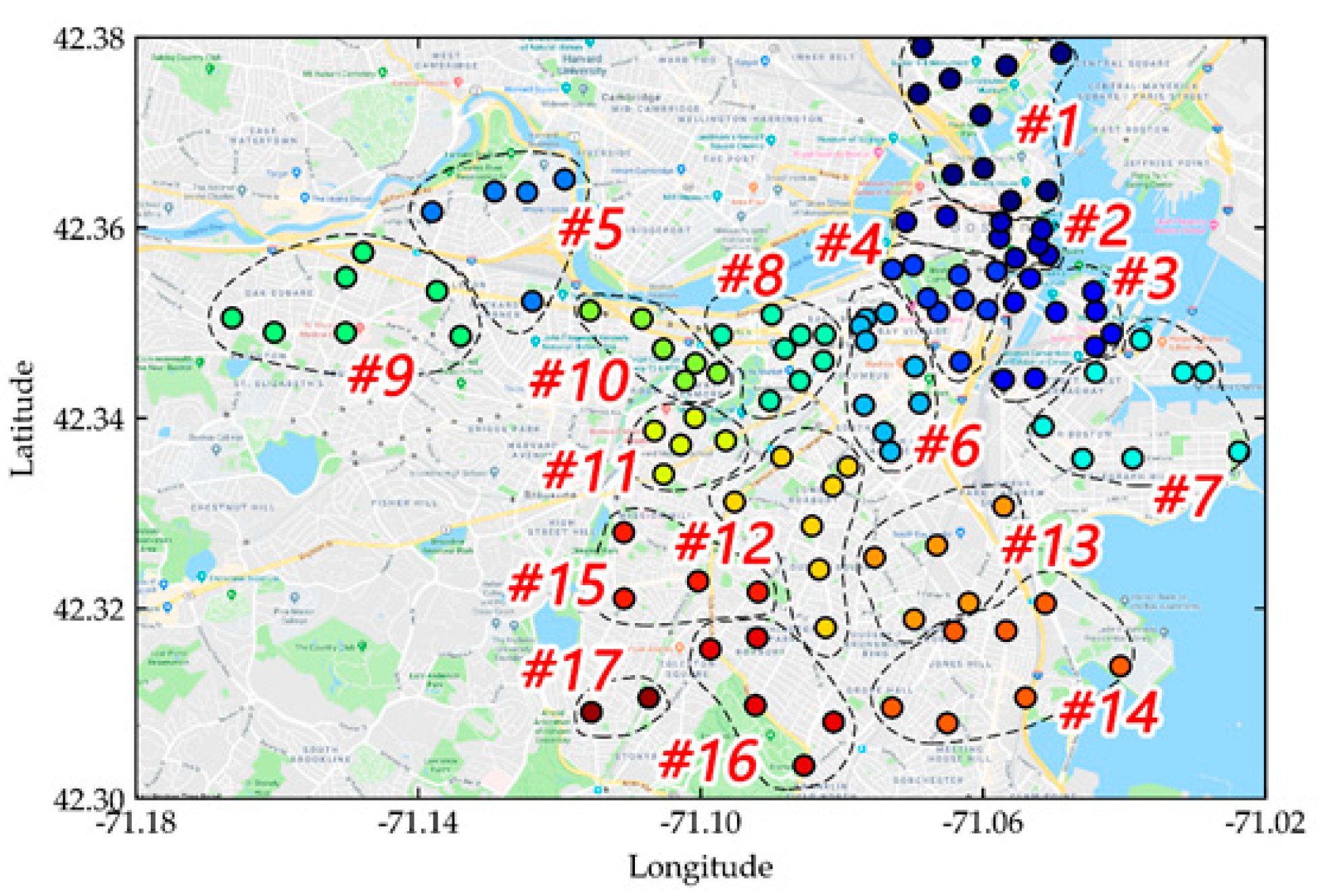
| Area ID | Number of Stations | Station ID |
|---|---|---|
| #1 | 10 | 40, 47, 85, 129, 38, 98, 94, 190, 169, 171 |
| #2 | 8 | 43, 48, 151, 20, 23, 44, 6, 60 |
| #3 | 9 | 31, 24, 7, 64, 192, 22, 63, 150, 65 |
| #4 | 9 | 59, 49, 81, 35, 42, 54, 120, 58, 152 |
| #5 | 5 | 17, 29, 149, 15, 41 |
| #6 | 9 | 50, 134, 36, 16, 4, 25, 26, 39, 13 |
| #7 | 8 | 119, 146, 121, 135, 1336, 186, 163, 161 |
| #8 | 8 | 21, 55, 61, 52, 53, 33, 5, 46 |
| #9 | 7 | 37, 8, 207, 66, 175, 208, 174 |
| #10 | 6 | 45, 122, 32, 19, 10, 9 |
| #11 | 5 | 160, 3, 11, 14, 30 |
| #12 | 7 | 56, 200, 51, 12, 27, 196, 204 |
| #13 | 5 | 113, 138, 106, 199, 128 |
| #14 | 7 | 167, 130, 93, 203, 205, 173, 92 |
| #15 | 4 | 197, 131, 159, 125 |
| #16 | 5 | 201, 126, 170, 202, 162 |
| #17 | 2 | 133, 124 |
| Station ID | Station Capacity | Initial Inventory | Inventory Variation Rate |
|---|---|---|---|
| 31 | 15 | 13 | −1 |
| 24 | 19 | 5 | 2 |
| 7 | 15 | 6 | 1 |
| 64 | 19 | 14 | −1 |
| 192 | 19 | 2 | −1 |
| 22 | 46 | 7 | −4 |
| 63 | 15 | 8 | 0 |
| 150 | 19 | 2 | −1 |
| 65 | 19 | 14 | −3 |
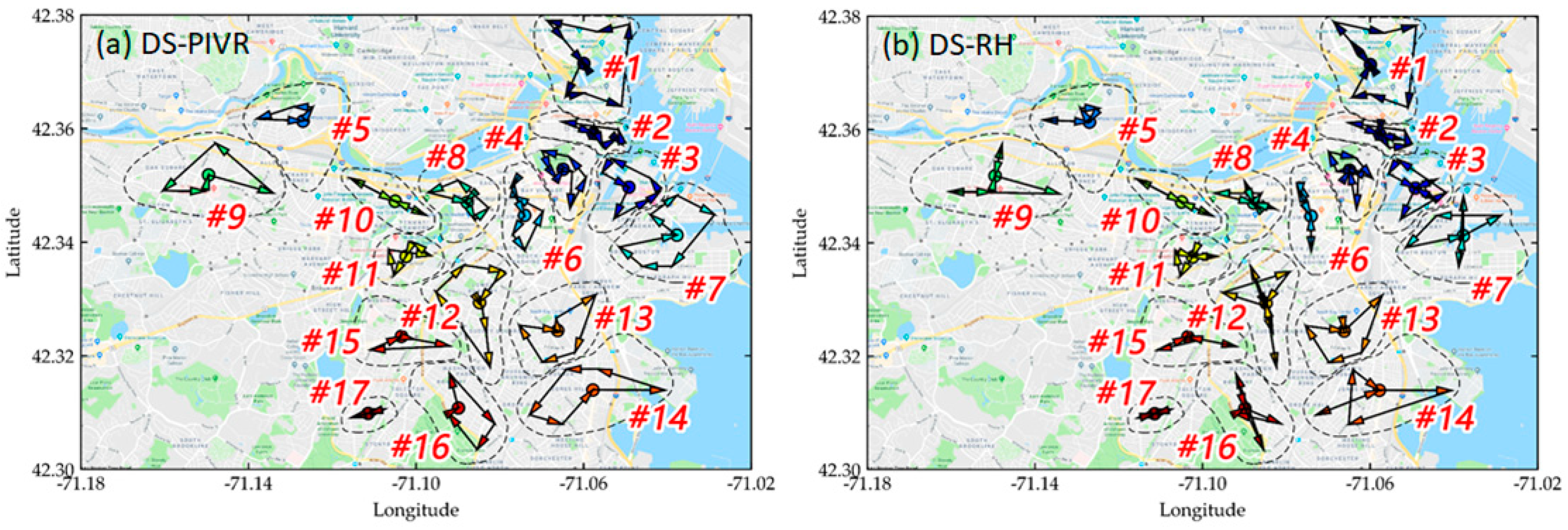
| Area ID | DS-PIVR | DS-RH | Reduction Ratio (%) | ||
|---|---|---|---|---|---|
| Route | Distance | Route | Distance | ||
| #1 | 0→98→190→38→40→85→129→169→94→0 | 6345.50 | 0→98→169→129→85→40→38→190→0→94→0 | 7468.62 | 15.04 |
| #2 | 0→44→48→151→43→20→6→0 | 3180.53 | 0→48→43→20→6→0→151→0→44→0 | 4045.74 | 21.39 |
| #3 | 0→150→65→31→24→192→22→0 | 3822.97 | 0→150→31→192→22→0→65→0→24→0 | 5666.36 | 32.53 |
| #4 | 0→81→152→59→54→120→42→49→0 | 3502.15 | 0→42→120→54→59→0→49→0→81→152→0 | 4346.82 | 19.43 |
| #5 | 0→29→149→15→0 | 2386.70 | 0→15→0→149→29→0 | 2861.84 | 16.60 |
| #6 | 0→25→39→4→16→134→36→0 | 3300.59 | 0→134→16→0→39→0→36→0 | 3962.96 | 16.71 |
| #7 | 0→163→186→135→119→121→161→0 | 5767.28 | 0→135→163→161→0→186→119→0 | 6919.33 | 16.65 |
| #8 | 0→52→55→46→21→53→33→0 | 3499.60 | 0→52→33→0→55→21→0→53→0 | 3835.56 | 8.76 |
| #9 | 0→66→37→174→175→0 | 5368.51 | 0→66→174→175→0→37→0 | 5924.42 | 9.38 |
| #10 | 0→9→19→45→0 | 3316.31 | 0→45→19→9→0 | 3316.31 | 0.00 |
| #11 | 0→30→11→160→3→0 | 2564.48 | 0→30→11→0→3→0→160→0 | 2923.58 | 12.28 |
| #12 | 0→56→204→196→27→12→51→200→0 | 5419.80 | 0→56→27→51→0→12→204→0→196→0 | 8542.36 | 36.55 |
| #13 | 0→138→113→128→199→106→0 | 4635.72 | 0→113→128→199→106→0→138→0 | 5003.24 | 7.35 |
| #14 | 0→92→167→130→203→205→0 | 6132.41 | 0→92→205→130→0→203→0 | 7942.72 | 22.79 |
| #15 | 0→131→197→125→0 | 3201.65 | 0→131→125→0→197→0 | 3763.64 | 14.93 |
| #16 | 0→201→202→170→162→0 | 3762.74 | 0→202→162→0→170→201→0 | 5110.39 | 26.37 |
| #17 | 0→124→133→0 | 1372.87 | 0→124→0→133→0 | 1372.87 | 0.00 |
| Case | Number of Settings with MIP Solution | Reduction Ratio Among All Areas | Reduction Ratio for the Whole PBS | ||
|---|---|---|---|---|---|
| Best Found | Average | Best Found | Average | ||
| Boston | 33 | 62.25% | 13.68% | 21.06% | 16.93% |
| Washington DC | 36 | 74.70% | 10.66% | 17.26% | 14.37% |
© 2019 by the authors. Licensee MDPI, Basel, Switzerland. This article is an open access article distributed under the terms and conditions of the Creative Commons Attribution (CC BY) license (http://creativecommons.org/licenses/by/4.0/).
Share and Cite
Gao, L.; Xu, W.; Duan, Y. Dynamic Scheduling Based on Predicted Inventory Variation Rate for Public Bicycle System. Sustainability 2019, 11, 1885. https://doi.org/10.3390/su11071885
Gao L, Xu W, Duan Y. Dynamic Scheduling Based on Predicted Inventory Variation Rate for Public Bicycle System. Sustainability. 2019; 11(7):1885. https://doi.org/10.3390/su11071885
Chicago/Turabian StyleGao, Liang, Wei Xu, and Yifeng Duan. 2019. "Dynamic Scheduling Based on Predicted Inventory Variation Rate for Public Bicycle System" Sustainability 11, no. 7: 1885. https://doi.org/10.3390/su11071885
APA StyleGao, L., Xu, W., & Duan, Y. (2019). Dynamic Scheduling Based on Predicted Inventory Variation Rate for Public Bicycle System. Sustainability, 11(7), 1885. https://doi.org/10.3390/su11071885