Influent Forecasting for Wastewater Treatment Plants in North America
by
 ,
,
Gavin Boyd
1,†, 
Dain Na
1,†,
Zhong Li
1,*,
Spencer Snowling
2,
Qianqian Zhang
1,3 and
Pengxiao Zhou
1 1
Department of Civil Engineering, McMaster University, Hamilton, ON L8S 4L7, Canada
2
Hydromantis Environmental Software Solutions, Inc., 407 King Street West, Hamilton, ON L8P 1B5, Canada
3
School of Management, Chengdu University of Information Technology, Chengdu 610225, China
*
Author to whom correspondence should be addressed.
†
Joint first authors.
Sustainability 2019, 11(6), 1764; https://doi.org/10.3390/su11061764
Submission received: 20 January 2019
/
Revised: 16 March 2019
/
Accepted: 17 March 2019
/
Published: 23 March 2019
(This article belongs to the Special Issue Rural Sustainable Environmental Management)
Abstract
:Autoregressive Integrated Moving Average (ARIMA) is a time series analysis model that can be dated back to 1955. It has been used in many different fields of study to analyze time series and forecast future data points; however, it has not been widely used to forecast daily wastewater influent flow. The objective of this study is to explore the possibility for wastewater treatment plants (WWTPs) to utilize ARIMA for daily influent flow forecasting. To pursue the objective confidently, five stations across North America are used to validate ARIMA’s performance. These stations include Woodward, Niagara, North Davis, and two confidential plants. The results demonstrate that ARIMA models can produce satisfactory daily influent flow forecasts. Considering the results of this study, ARIMA models could provide the operating engineers at both municipal and rural WWTPs with sufficient information to run the stations efficiently and thus, support wastewater management and planning at various levels within a watershed.
1. Introduction
Predicting wastewater influent flow is important economically, environmentally, and socially. Forecasting influent flow at wastewater treatment plants (WWTPs) can benefit the operators, as well as the plant itself. With reliable predictions forecasted in advance, operators can run the plant efficiently, which could support wastewater management and planning at various levels within a watershed [1,2].
Unlike hydrological forecasts, forecasting wastewater flow rates has not been researched to a large extent. There are no well-established wastewater influent forecasting tools available to WWTPs operators and managers. Traditionally, operators must rely on their knowledge to forecast ahead, or possibly use extensive complex physical models which can be difficult to tune and monitor [3]. In the past decade, to better predict wastewater characteristics, a few models were developed. For example, Kim et al. (2015) used the k-nearest neighbor (k-NN) method to predict various wastewater qualities such as chemical oxygen demand (COD), suspended solid (SS), total nitrogen (TN), as well as total phosphorus (TP) [3]. Additionally, Nadiri et al. (2018) combined the Artificial Neural Network (ANN) model with the fuzzy logic time series models and used a supervised committee fuzzy logic (SCFL) model to predict various wastewater effluent quality parameters [4]. Moreover, Ottmar et al. (2013) used the mass balance-based model to predict the concentrations of pharmaceuticals entering WWTPs in the United States [5]. The model concluded to be adequate to provide rough predictions of the drug influent concentrations, however some factors were speculated to have caused inaccuracy in the prediction results.
Amongst the multiple forecasting models available, time series models have been widely used as they only depend on internal data to make their prediction [3]. For example, only the previous flow data would be needed to forecast the future flow predictions. The autoregressive integrated moving average (ARIMA) model is a well-developed time series model that can be dated back to 1955 [6]. In 1970, Box and Jenkins made several contributions to the ARIMA model [7]. Ever since, it has been used in many different fields to analyze time series and forecast future data points. For example, Santamaria-Bonfill et al. (2015) proposed an ARIMA model to predict wind speed [8]. Moreover, in 1998, ARIMA was used to forecast monthly tourism in Singapore, China [9]. ARIMA has also had a significant impact on hydrological modelling. Wang et al. (2015) made use of ARIMA to formulate long-term annual runoff predictions for three reservoirs in China [10]. The ARIMA model was integrated with an ensemble empirical mode decomposition (EEMD) to improve the model’s accuracy. Fifty years of the datasets were used to train the model, then approximately 10 years of data were used for validation purposes. Similarly, annual runoff predictions were made for two reservoirs in China using a hybrid ARIMA model with Singular Spectrum Analysis (SSA) [11]. The datasets were first split into 45 and 46 years of training sets and then the 12 years remaining were used to validate the model. SSA was used to extract trends and periodicities in the 45 and 46 years of the training data from the two reservoirs. Once these subsets of data were created, ARIMA modelled each and superimposed the subseries together to produce a 12-year forecast. Another dam reservoir forecast was produced to predict monthly inflow discharge into the Dez dam [12]. The 47-year dataset was split into 42 years for training and the last five years for validating the three different models [12]. The root mean square error (RMSE) was used to compare the seasonal ARIMA, ARMA (Autoregressive Moving Average), and the artificial neural network (ANN). It was discovered that the seasonal ARIMA model was the most effective for monthly forecasts up to twelve months. Furthermore, larger scale studies which evaluated the performance of ARIMA can be found in [13]. Models derived from the Autoregressive Moving Average (ARMA) families and machine learning black box methods, such as Neural Networks and Random Forests, were used to forecast monthly or annual hydrological processes, such as streamflow rates. In this study, it was found that both black box and stochastic models, such as ARIMA, provided accurate results according to their forecasting quality metrics, such as Mean Absolute Percentage Error and the Nash (NSE) Coefficient, for short time series forecasting. Another similar study by Papacharalampous et al. compared various stochastic and machine learning models to create one-step ahead annual forecasts for temperature and precipitation [14].
Particularly, there have been several studies on the application of ARIMA in wastewater prediction. Kim et al. (2006) used ARIMA to forecast COD, ammonia, phosphate, and flow rate [15]. Furthermore, wastewater influent flow was predicted by Chen et al. (2014) using the autoregressive moving average (ARMA) model to provide efficient chemical dosing for the effluent [16]. These studies demonstrated ARIMA’s great potential in predicting wastewater characteristics. However, the performance and reliability of ARIMA to model daily wastewater influent flowrate forecasts have not been extensively tested. Given the promising potential of ARIMA for solving water and wastewater prediction problems, it is desired that ARIMA be further demonstrated in the field of wastewater treatment inflow.
Therefore, the objective of this study is to propose an influent flow forecasting tool for WWTPs using the ARIMA model and test ARIMA’s performance using multiple WWTPs in North America. Wastewater inflow data will be collected from five stations across North America (Woodward, Niagara, North Davis, and two confidential plants), in order to train and validate the ARIMA model. Different statistical criterions, including RMSE, MAPE, and R-squared, will be used to evaluate the performance of the ARIMA model. This study will provide important technical support for improving the design, operation, and management of WWTPs. The rest of the paper is structured as follows: Section 2 presents the model structure and evaluation criterions. Section 3 introduces the five selected WWTPs and the data collection process. Section 4 presents the modeling results. Section 5 provides a discussion regarding ARIMA’s advantages and disadvantage, as well as potential future research. Section 6 summarizes the major findings of this study.
2. Methodology
2.1. Autoregressive Integrated Moving Average (ARIMA)
ARIMA is an approach that seeks to predict future behavior from an examination of the previous history of the series itself [14]. The early form of ARIMA originated in 1955 [6]. It is worth mentioning that a more precise definition should use the “ARIMA (p, d, q)”, where parameter p is the order of the autoregressive (AR) model, parameter d is the degree of differencing, and parameter q is the order of the moving-average (MA) model. However, the model is denoted as ARIMA in this paper for simplicity. According to Box et al. (2015), the general form of the ARIMA model is given as Equation (1).
where is a constant; is a normal stationary stochastic process, called the white noise process; is the discrete time series value at time ; B is a backward shift operator that gives ; is the nonstationary autoregressive operator with d of the roots of equal to unity; is the stationary autoregressive operator and ; is the moving average operator and . and are the autoregressive and moving average coefficients, respectively. The readers are referred to Box et al. (2015) and Tyralis and Papacharalampous (2017) for a more detailed definition of ARIMA [17,18].
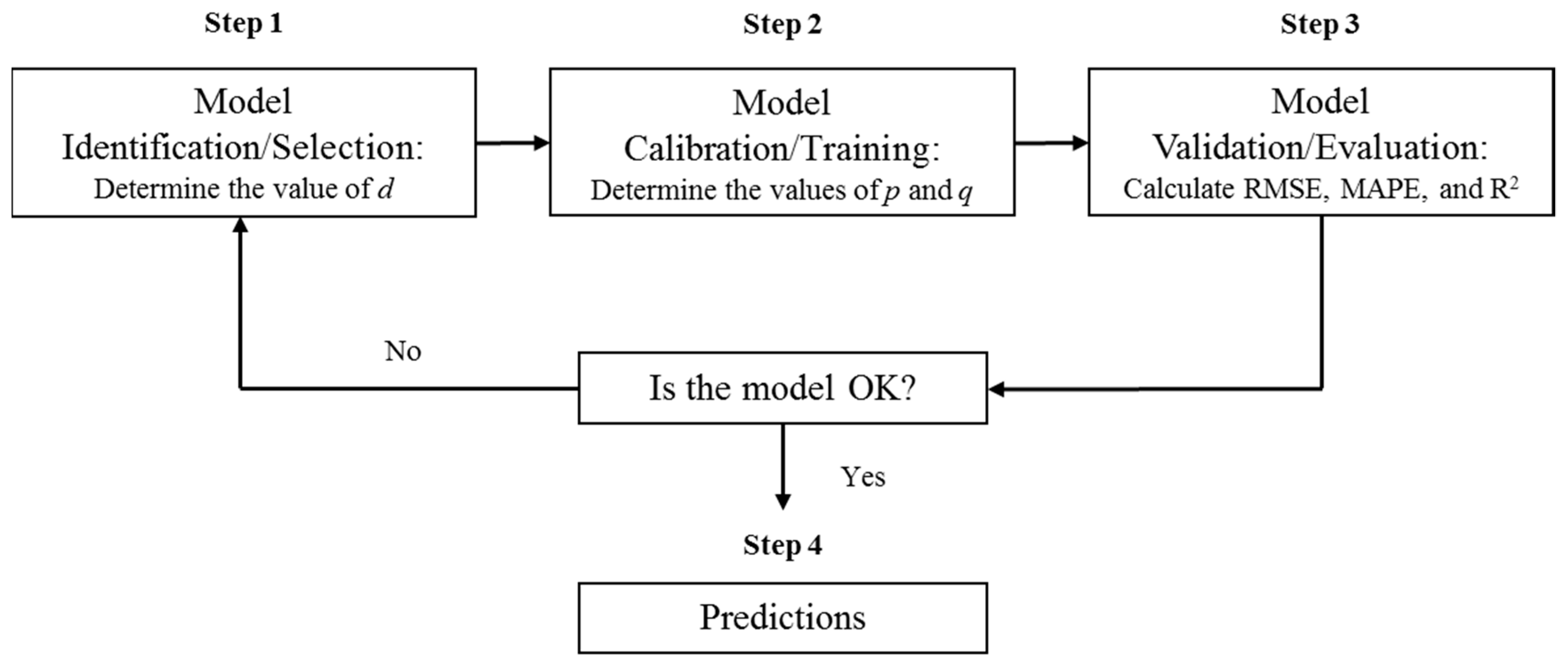
Box and Jenkins (1970) created the building blocks of ARIMA, breaking down the prediction process into three iterative steps: identification, estimation, and validation—as seen in Figure 1 [3,19,20]. The Integration value (d) is found in the identification process. The estimation step includes finding the ARIMA parameters and coefficients from the training set. Then, the model can be validated by running the full time series using the best training (p, d, q) values. Box and Jenkins’ model was later used by many researchers to forecast time series as forecasting became the fourth step in the Box-Jenkins approach.
There have been numerous technological and methodological innovations to improve ARIMA’s forecasting abilities, such as outlier detection and Kalman filtering. Detecting outliers can help improve the forecasting results as the abnormal variation within the data would decrease [21]. Furthermore, outliers can be detected either before the forecasting process by analyzing the input data or after the forecast is produced by comparing the forecasted values with the observed values. Liu et al. (2001) used outlier detection for their time series analysis on a fast-food restaurant [22]. ARIMA was utilized to predict the daily demand for a product sold at a particular restaurant. After the ARIMA forecast, eight outliers were detected by comparing the predicted results with the observations. Finding the outliers proved to be beneficial to the restaurant owner as majority of them were related to holidays and extreme weather events. Hence, in this case, outlier detection led to the discovery of certain patterns in datasets. However, the difficulty surrounding outliers is determining whether or not that data point is an outlier that can be deleted, or an extreme value that would be important to keep. As explained in the fast-food restaurant case, those outliers deemed to be extreme values that helped the owner detect a trend. However, there could be cases where the outliers would be best removed to increase the model’s performance.
2.2. The ARIMA Model for Influent Forecasting
To build an ARIMA model for daily influent prediction, resampling of the data was necessary depending on the frequency of the data in each WWTP. If the data was observed multiple times in a day, it was averaged to daily frequency. The next step of the Box-Jenkins process is the identification stage. The autocorrelation (AC) and partial autocorrelation (PAC) graphs were used to determine if there were any signs of trends within the series [20]. If they exist in the series, a higher order of differencing would be needed until the series appears to lose any trends. When no trends are present in the series, the AC and PAC graphs quickly converge to zero, meaning that particular value of (d), which denotes the number of times that the observation data are differenced, can be determined for the ARIMA model.
Then, the dataset was split into two sections. Two-thirds of the data was used for the training of the model, whereas one-third of the data was used for the validation of the model. For the training set, three parameters, including p, d, and q, were configured manually. The integrated value d was first found in the identification process, then a number of (p, q) sets were searched using a grid search algorithm. For each (p, q) set, the other coefficients in the ARIMA model were estimated with fixed p, q, d values. The optimal (p, d, q) combination would be found by choosing the set with the lowest root mean square error (RMSE). Searching for the optimal combination of (p, d, q) could help calibrate the model for best performance; however, it is worth mentioning that exploring all combinations in a large subset of integer values may leave the model prone to overfitting. The higher the values of p and q, the higher the number of parameters. An ARIMA model with a large number of parameters normally has a lower generalization ability. Therefore, careful selection of p and q is suggested. In this study, models with high number of parameters would not be penalized, which is not ideal. Certain procedures to penalize overfitting should also be considered when the values of p and q are high [23].
Once the best combination of (p, d, q) was found and the other coefficients were calibrated, the model could be finalized and loaded to make one-step ahead predictions for the testing period. The authors are referred to Box et al. (2015) for detailed forecasting procedures. The loaded model was used directly for the whole testing period, which means the predictions were not made in a roll-forecast manner and the model was not updated with observations for each time step. In this study, no forecasts were generated beyond the testing period because the main purpose of this work is demonstrating ARIMA’s forecasting capability, rather than generating actual forecasts for the five WWTPs.
2.3. Model Evaluation
There are a number of error measures that could be used for making comparisons between observed and predicted time series. Since no one measure is superior on all criteria, multiple measures, including RMSE, Mean Absolute Percentage Error (MAPE), and coefficient of determination (R-squared), were used for model evaluation [24].
In order to choose the best (p, q) set, the combination with the lowest RMSE was used. RMSE is the square root of the average of square differences between the actual and predicted values at specific timestamps. Since RMSE describes the magnitude of the error which could be useful to decision makers, it has been frequently used for evaluating the accuracy of a forecasting method [24]. It can be calculated as in Equation (4) below.
where yj is the actual value, is the predicted value, and n is the total number of data points [25].
RMSE depends on a few different factors. First, RMSE depends on the units and the frequency of the dataset, meaning it cannot be absolutely defined as a good or bad value [24]. If the RMSE is the same as the standard deviation, the ARIMA model would only be as accurate as using the mean as the prediction. Hence, if the RMSE value is lower than the standard deviation, it implies that the ARIMA model better predicts the data compared to using the mean as the prediction. To continue, RMSE also depends on the variance between the actual and predicted values because the difference is squared. Therefore, the primary benefit of RMSE is that it gives high weights to larger deviations, which in return, represents a better model performance [25]. However, a disadvantage includes the fact that outstanding outliers can heavily skew the RMSE results and show a misleading model performance [24].
MAPE has also been used widely in scientific research as it is simple to use [26]. MAPE was not used for the calibration of the ARIMA model, however it was used for model evaluation in the validation process. MAPE is the mean of the individual theoretical errors calculated at each timestamp, as seen in Equation (5) [23]. Hence, lower MAPE values infer better model performance.
The coefficient of determination (R-squared) is another error criterion which was used for model validation. R-squared has been used frequently for model evaluation. It is a statistical measure which represents the ability of the independent variable (observed) to predict the variations of the dependent variable (predictions). Therefore, the correlation is between the line of best fit and the predicted values [27]. The closer the R-squared is to the value of one, the better the model has performed as there is less error variance [28]. The opposite is said to be as the R-squared approaches zero. In general, an R-squared value greater than 0.5 is acknowledged as being acceptable [28]. As seen in the Equation (6) below, R-squared is the sum of the distance between the predicted value and the linear line, divided by the sum of the distance between the predicted value and the mean of predictions [29].
3. Study Area and Data Collection
3.1. Selected Wastewater Treatment Plants
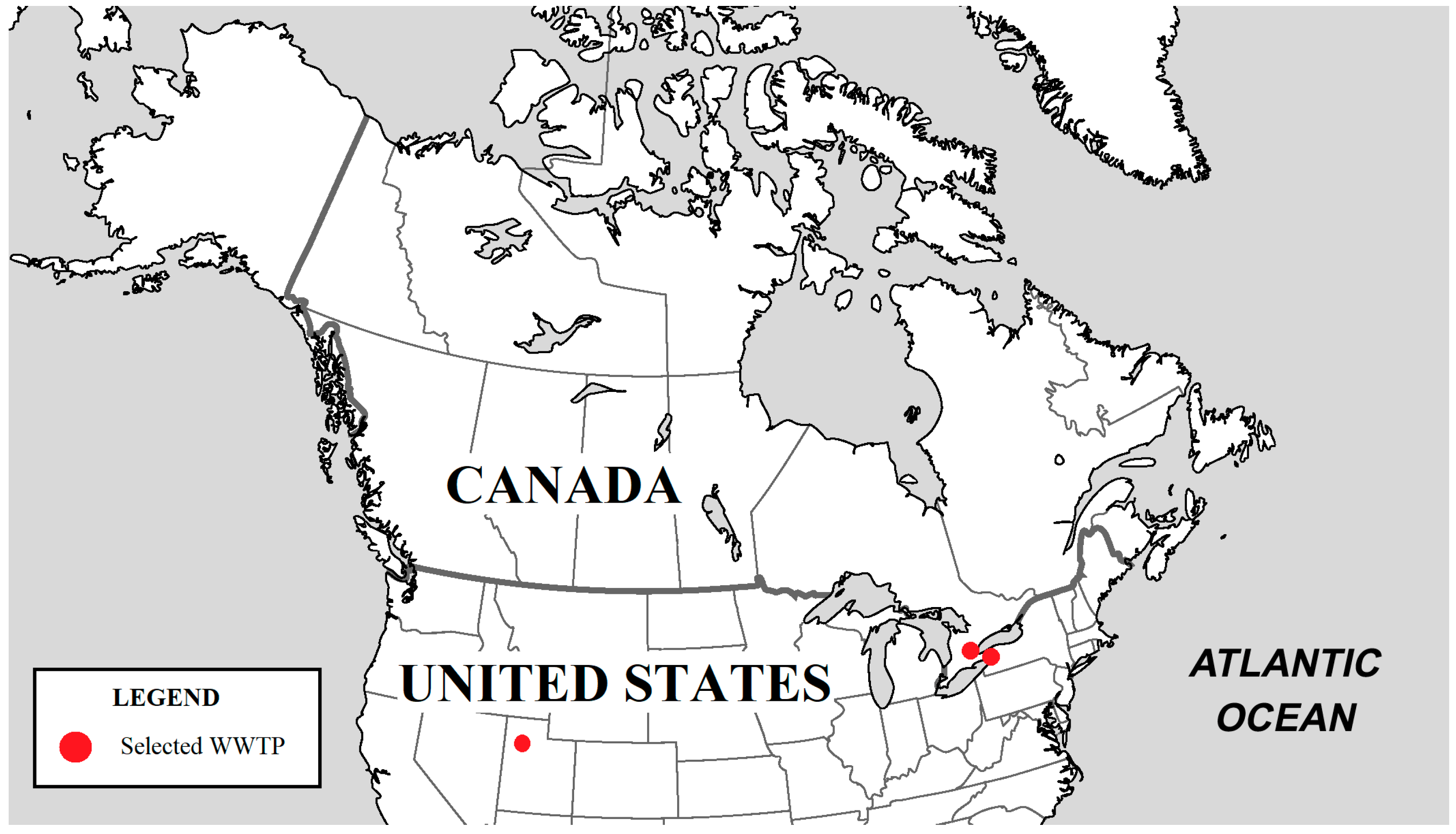
The five WWTPs used to test the ARIMA model in this study include the following stations: Woodward (Canada), North Davis (United States), Niagara (Canada), Confidential Plant I, and Confidential Plant II. The approximate location of each treatment plant (except the two confidential plants) is shown in Figure 2.
Woodward Avenue Wastewater Treatment Plant is one of the two WWTPs located in the City of Hamilton, Ontario, Canada. Hamilton has a total area of 1117 km2 and a population of approximately 536,900 [30,31]. As Hamilton is an older city, some regions still use combined sewer systems. Woodward Avenue WWTP treats both sanitary and combined sewage, with an average capacity of 4.73 m3/s. At this plant, five wastewater treatment processes occur: preliminary treatment, primary treatment, secondary treatment, effluent disinfection, and sludge digestion. Currently, an upgrade project is occurring at Woodward Avenue WWTP and is expected to be completed in 2022. With this project, an additional new third level of treatment will occur in the wastewater treatment process [31].
The North Davis Sewer District WWTP in Utah serves the area extending from Roy to Kaysville (North to South) and from Wasatch Mountains to the Great Salt Lake (from East to West) [32]. The District covers about 207 km2 of area which is populated with an estimated 200,000 people. Each city in the area has its individual sewage collection lines; however, they are discharged into the larger District lines. The treatment plant can treat 34 million gallons of wastewater each day and discharges the treated water into the Great Salt Lake. The process at the North Davis plant includes the following: wastewater collection, pretreatment, headworks, primary treatment, secondary treatment, disinfection and effluent, solids treatment, as well as cogeneration of products. The products from the treatment process include biosolids, which are used as a source of organic soil amendment and fertilizer, electricity, and heat [32].
The WWTP in the Niagara Region is situated in Crystal Beach, a town of roughly 11 km2 [33]. The population of Crystal Beach in 2016 was found to be about 8500 people, a 5.8% increase from 2011. The two confidential WWTPs are located in North America. Currently, the detailed locations of these plants cannot be disclosed.
3.2. Data Collection
The data for this study was provided by Hydromantis. Hydromantis is a company from Hamilton, Ontario, Canada that focuses on wastewater and hydraulic aspects of environmental engineering, as well as the development of wastewater modelling and simulation software. Each WWTP varies in the time period that the data was collected, the data frequency, and the flow unit. These variations between the WWTPs was not significant in affecting the individual WWTP results as they were tested separately. Although the data for each station was collected at different periods of time, it is still consistent in the context of this study as each individual data set was split to use two-thirds for calibration and one-third for validation, regardless of the data collection time period. The details of data collected for each WWTP are given in Table 1 where MLD refers to millions of liters per day and MGD refers to millions of gallons per day. The missing values of the confidential plants in Table 1 do not affect the results of the study as they were not used to train or test the data.
4. Results
4.1. Characterization of the Influent Time Series
The wastewater influent flow rate shows many different patterns for each WWTP. Due to the diverse social and environmental factors, such as population in the surrounding area, land use, collection system, and climate conditions, each WWTP hosts a unique dataset. Despite the many differences that each geographical area encompasses, each plant’s flow rate has a general tendency to rise into spring and decrease towards the summer. This commonality can be explained by more frequent and intense rainfalls in the springtime, combined with snowmelt.
Confidential Plant II’s flow data follows a general increasing trend from November 2015 to the maximum peak in April 2016. Afterwards, it decreases to a minimum towards the fall and winter of 2016, as seen in Figure 3a. As for the flow at Woodward WWTP, it varies significantly within each month, as seen in Figure 3b. Since ARIMA does not use any information from exogenous variables, such as precipitation and snowmelt, variations in these variables cannot be well captured, which generally lowers ARIMA’s forecasting accuracy. The flow data from Niagara’s WWTP is observed in Figure 3c. It shows a steady rise in flow rate from October 2016 to April 2017 as it approaches the peak flow. In both 2016 and 2017, the minimum flow rate occurs around August. Additionally, the flow rate is greater in 2017 in comparison to 2016. Figure 3d represents the flow in North Davis WWTP. The flow is fairly constant throughout 2016 from June to October. A high peak is seen at the end of February 2017 and low flows are observed in the winter of 2016. Unlike the other WWTPs, North Davis does not show any seasonal patterns throughout 2016, such as an increase in spring and a decrease in summer. This may be due to the lower amounts of precipitation in the winter of 2016. For Confidential Plant I, it is observed from Figure 3e that the highest peak flow occurs in March 2016. However, large flow rates occur in the winter of 2015 and 2016 as well. There is a steady decrease in flow through the spring and into the summer, while a steady increase begins in the fall.
The weekly and seasonal patterns of hourly inflow rate were also analyzed and the patterns at Confidential Plant II are presented in Figure 4 as an example. As shown in Figure 3a, there are many local peaks within each month. The local peaks most likely result from an increase in flow rate throughout the week and into the weekend. This weekly trend can be seen in Figure 4. Figure 4 displays seven different lines which represent the flow rate for each of the days in a week. Typically, the flow rates are greater throughout the day on Saturday and Sunday.
Like many sets of data, outliers were present for this study. Outliers in the data were identified using professional judgement by the WWTP engineers. The engineers at each WWTP know the conditions of the plant, thus they were able to distinguish outliers from extreme values. Once the outliers were confirmed, they were deleted and replaced by a linearly interpolated value. Likewise, missing values or null values within the data collection were also deleted and filled using linear interpolation.
Furthermore, to ensure that the data for ARIMA analysis is stationary, the AC and PAC graphs were analyzed. The graphs for North Davis are presented in Figure 5 as an example. Since the flow frequency for North Davis was daily data, resampling for the AC and PAC graphs was not needed. A differencing value of one was used as both the AC and PAC graphs met all the criteria. They tended to zero, and most of the correlations remained within the confidence limits, as seen in Figure 5b. However, when the differencing value was zero (Figure 5a) or two (Figure 5c), the AC and PAC graphs did not satisfy the two criteria.
4.2. Prediction Results
The ARIMA model for each WWTP was calibrated using two thirds of the flow data. Based on the calibration results, a different set of (p, d, q) was selected for each WWTP. Table 2 shows the results for each error criterion, and Figure 6 shows the model prediction graphs for each plant.
Overall, three error criterions were used to evaluate the model’s performance: RMSE, MAPE, and the coefficient of determination. RMSE was only used to calibrate the model, however all three were used in the validation portion. All three can be used in unison to piece together the quality of the prediction as each criterion provides different error perspectives—as explained in Section 2.3. Although RMSE is widely accepted as an effective model evaluation criterion, it has a primary disadvantage which is that RMSE is a relative error. RMSE depends on both the flow units and the frequency of which the data was taken. The larger flow units would result in larger RMSE values. This makes it harder to absolutely define the quality of the predictions. For example, Niagara’s RMSE was roughly 0.01 m3/s, whereas Woodward’s was approximately 0.58 m3/s. As seen in Figure 6b,c, despite the disadvantage of RMSE being a relative error, the RMSE values can be compared to the standard deviations at each station, as explained in Section 2.3. The RMSE values for each of the five stations are at least two times less than the standard deviation, as displayed in Table 1 and Table 2. Since the RMSE for each station is less than its respective standard deviation, it is observed that the ARIMA model provides good forecasts [14].
MAPE was another criterion used to measure the quality of the results from the ARIMA model. As seen by Equation (5) in Section 2.3, the results are considered to be better if the MAPE value is closer to zero [26]. For example, Confidential Plant II results present low MAPE values for both the calibration and prediction periods. This means that by the definition of MAPE, Confidential Plant II’s results are more satisfactory compared to a station such as Niagara. However, a disadvantage of using MAPE is the fact that the results can be skewed if there are zero values or values close to zero in the dataset [23]. This is because dividing by such a small value will increase MAPE tremendously, especially if the value of the numerator is large [26]. A result of this, drawback can be seen in the result for Niagara WWTP. Referring to Figure 6c at approximately Day 575 on the x-axis (the end of July 2017), a significant difference can be observed between the actual and the predicted values. At this time, however, the actual value is relatively small. Thus, dividing a large difference by a small value will increase and skew the MAPE value. This may be one of the reasons why Niagara’s MAPE performance was poor.
R-squared was used to determine the performance of the model. As explained in Section 2.3, the coefficient of determination describes how well the observed values predict the variance of the forecasted results. A perfect forecast would result in the coefficient of determination being one, while a value of zero would indicate that there is no correlation between the observed and predicted. As seen in the results displayed in Section 3.2, Niagara has the worst testing coefficient of 0.557, whereas North Davis has the best, which is 0.898. Therefore, Niagara’s and North Davis’ observed values can account for, respectively, 55.7% and 89.8% of the predicted variances. The R-squared results for all the stations in this study are greater than 0.5, meaning the results are satisfactory [23].
5. Discussion
Despite the few drawbacks that ARIMA possesses, ARIMA has proven to be a reliable model for hydrological purposes, such as flow forecasting. A Seasonal ARIMA (SARIMA) model combined with ANN was used to forecast monthly inflow into the Jamishan dam reservoir in West Iran [34]. The model produced exemplary coefficient of determination results. The SARIMA model chosen had a testing R-Squared of 0.579, which is greater than 0.5 [34]. Another study in Seoul, South Korea used ARIMA to predict seasonal urban water consumption based on weather variables such as temperature, precipitation, wind speed, relative humidity, as well as cloud cover [35]. The average R-squared value was found to be 0.479 [35]. Comparing to these two examples, this study demonstrates that ARIMA can be considered a reliable forecasting model, especially with longer temporal resolutions. An extensive test of ARIMA and 11 other stochastic methods regarding their streamflow forecasting properties can be found in [13].
Like all models, the ARIMA model has advantages as well as disadvantages. Some advantages that ARIMA possess includes the fact that it is a simplistic model which can be interpreted and calculated fairly easily. Machine learning models like ANN cannot be manually interpreted with simple calculations as one can do with ARIMA. To continue, while most data-driven models typically use information from exogenous variables, no weather data is needed for ARIMA to make its prediction [13,36,37]. This is beneficial as not all historical weather data is accurate or even exists, especially higher frequency data. High temporal resolution weather data including precipitation can be extremely hard to obtain. For instance, Environment Canada’s daily historical weather data consists of many files with plenty of missing data points. ARIMA avoids these issues as it only requires internal inputs to forecast [17,38]. The abovementioned advantages of ARIMA make it a reliable and effective tool for WWTPs managers. In this study, ARIMA is successfully applied to the forecasting of wastewater influent rate at five WWTPs in North America. To the authors’ knowledge, this is the first time that ARIMA has been tested for wastewater influent forecasting to a large extent.
Although the ARIMA model has many advantages, it also has some drawbacks. To begin, ARIMA does not use information from exogenous variables, which leads to a limit of predictability. Including relevant data as model input, such as precipitation and snowmelt, could sometimes help address this problem [39]. When weather forecasts are used as model input for wastewater influent forecasting, it is important to ensure the accuracy/quality of the weather forecasts. Meanwhile, ARIMA can only run a continuous time series, meaning the missing values in the dataset must be filled in. It can be a long process to find and calculate all the absent values, meaning it will require more time to prepare the data to run the model. Also, filling in missing values using linear interpretation can decrease the model performance as the variations in the data may be incorrectly represented [7]. It is recommended that users carefully process wastewater data and ensure data quality when using ARIMA for influent forecasting. However, it should be noted that the presence of missing values will influence the performance of many other forecasting methods, not just ARIMA. Moreover, one of ARIMA’s assumptions is that there is no periodicity in the data. The model accuracy may be affected when this assumption is not satisfied, which is not unusual in flow forecasting problems. Additionally, since the random shocks at each point of the time series are assumed to come from the same distribution, typically a normal distribution, ARIMA is not designed to predict extreme values [17]. WWTPs are suggested to closely monitor extreme weather conditions so that they can be prepared for extreme influent flows. Finally, running the model itself can be time consuming. There are existing procedures for fast parameter estimation for the ARIMA(p, d, q) [23,40]. In future applications, the practitioners are recommended to use such techniques to improve the efficiency of this model and to save computational time.
6. Conclusions
In this study, a daily influent flow forecasting model was proposed based on ARIMA. The performance and reliability of the ARIMA model was tested at five WWTPs across North America, including Niagara, Woodward, North Davis, and two confidential plants. The data used for each station varied in flow frequency, where some stations gathered data daily, while others measured in 5- or 15-min intervals. Each model was calibrated using RMSE as the error criterion to find the best combination of (p, d, q). Once the best combination was found, the prediction portion of the data was used to validate the model. The results for the calibration and validation set were each analyzed through the calculation of RMSE, MAPE, and R-squared. The R-squared values at all five station are higher than 0.55 during the validation period, and the RMSE for each station is less than its respective standard deviation. The results demonstrated that ARIMA can be used by WWTPs to forecast influent flow rate.
This study can provide valuable technical support for the prediction of influent characteristics at WWTPs, helping wastewater engineers to make the maximum use of the existing and future wastewater treatment facilities. ARIMA relies only on historical data and no external data to provide forecasts. Our results show that time series analysis based on ARIMA can be extremely advantageous for the plant operators to manage the plant economically, as well as for the local society and the surrounding environment.
A limitation of this study was the fact that only one error criterion was used to calibrate the model [41]. To improve the forecasting results for future research, an integrated function can be built to incorporate multiple error criterions such as RMSE, R-squared, MAPE, MAE, NSE, and many more. Meanwhile, the proposed ARIMA model is prone to overfitting as no penalizations were set in order to avoid high order of parameters during calibration. Additionally, as daily flow data may be characterized by occasional extreme values or intermittency, it is possible that nonlinear models rather than ARIMA, such as neural networks, could work better for forecasting purposes; however, studies show that stochastic methods like ARIMA and nonlinear machine learning methods may produce equally useful forecasts for geophysical processes [13]. In future studies, the ARIMA model can be combined with other methods to improve the accuracy of the forecasts, such as the ensemble empirical mode decomposition (EEMD) [42]; although, it is worth mentioning that some researchers are skeptical about hybrid techniques and believe a universally best techniques simply does not exist [43]. Results can also be improved by ensuring quality data is provided for the ARIMA model [2,44]. Finally, although ARIMA has been tested for five WWTPs in this study, more testing is still expected to further demonstrate the reliability of this approach.
Author Contributions
Conceptualization, Z.L. and S.S.; Data curation, S.S. and Q.Z.; Formal analysis, G.B., D.N., and P.Z.; Funding acquisition, Z.L. and S.S.; Investigation, Z.L. and P.Z.; Methodology, Z.L., Q.Z., and P.Z.; Project administration, Z.L.; Supervision, Z.L. and S.S.; Validation, G.B., D.N., and P.Z.; Visualization, Q.Z.; Writing—original draft, G.B. and D.N.; Writing—review & editing, G.B., D.N., Z.L., S.S., Q.Z., and P.Z.
Funding
This research was supported by the Southern Ontario Water Consortium and the Natural Science and Engineering Research Council of Canada.
Acknowledgments
The authors would like to thank the engineers at Hydromantis and the five WWTPs for their contributions to this study.
Conflicts of Interest
The authors declare no conflict of interest.
References
- Zhou, Y.; Huang, G.; Zhu, H.; Li, Z.; Chen, J. A factorial dual-objective rural environmental management model. J. Clean. Prod. 2016, 124, 204–216. [Google Scholar] [CrossRef]
- Zhou, Y.; Yang, B.; Han, J.; Huang, Y. Robust Linear Programming and Its Application to Water and Environmental Decision-Making under Uncertainty. Sustainability 2019, 11, 33. [Google Scholar] [CrossRef]
- Kim, M.; Kim, Y.; Kim, H.; Piao, W.; Kim, C. Evaluation of the k-nearest neighbor method for forecasting the influent characteristics of wastewater treatment plant. Front. Environ. Sci. Eng. 2016, 10, 299–310. [Google Scholar] [CrossRef]
- Nadiri, A.A.; Shokri, S.; Tsai, F.T.C.; Moghaddam, A.A. Prediction of effluent quality parameters of a wastewater treatment plant using a supervised committee fuzzy logic model. J. Clean. Prod. 2018, 180, 539–549. [Google Scholar] [CrossRef]
- Ottmar, K.J.; Colosi, L.M.; Smith, J.A. Evaluation of a prediction model for influent pharmaceutical concentrations. J. Environ. Eng. 2013, 139, 1017–1021. [Google Scholar] [CrossRef]
- Yaglom, A. The correlation theory of processes whose nth difference constitute a stationary process. Matem. Sb. 1955, 37, 141–196. [Google Scholar]
- Tsay, R.S. Time series and forecasting: Brief history and future research. J. Am. Stat. Assoc. 2000, 95, 638–643. [Google Scholar] [CrossRef]
- Lahouar, A.; Slama, J.B.H. Wind speed and direction prediction for wind farms using support vector regression. In Proceedings of the 5th International Renewable Energy Congress (IREC), Hammamet, Tunisia, 25–27 March 2014; pp. 1–6. [Google Scholar]
- Chu, F.L. Forecasting tourism: A combined approach. Tour. Manag. 1998, 19, 515–520. [Google Scholar] [CrossRef]
- Wang, W.C.; Chau, K.W.; Xu, D.M.; Chen, X.Y. Improving forecasting accuracy of annual runoff time series using ARIMA based on EEMD decomposition. Water Resour. Manag. 2015, 29, 2655–2675. [Google Scholar] [CrossRef]
- Zhang, Q.; Wang, B.D.; He, B.; Peng, Y.; Ren, M.L. Singular spectrum analysis and ARIMA hybrid model for annual runoff forecasting. Water Resour. Manag. 2011, 25, 2683–2703. [Google Scholar] [CrossRef]
- Valipour, M.; Banihabib, M.E.; Behbahani, S.M.R. Comparison of the ARMA, ARIMA, and the autoregressive artificial neural network models in forecasting the monthly inflow of Dez dam reservoir. J. Hydrol. 2013, 476, 433–441. [Google Scholar] [CrossRef]
- Papacharalampous, G.; Tyralis, H.; Koutsoyiannis, D. Comparison of stochastic and machine learning methods for multi-step ahead forecasting of hydrological processes. Stoch. Environ. Res. Risk Assess. 2019, 33, 1–34. [Google Scholar] [CrossRef]
- Papacharalampous, G.; Tyralis, H.; Koutsoyiannis, D. One-step ahead forecasting of geophysical processes within a purely statistical framework. Geosci. Lett. 2018, 5, 12. [Google Scholar] [CrossRef] [Green Version]
- Kim, J.; Ko, J.; Im, J.; Lee, S.; Kim, S.; Kim, C.; Park, T. Forecasting influent flow rate and composition with occasional data for supervisory management system by time series model. Water Sci. Technol. 2006, 53, 185–192. [Google Scholar] [CrossRef]
- Chen, P.; Pedersen, T.; Bak-Jensen, B.; Chen, Z. ARIMA-based time series model of stochastic wind power generation. IEEE Trans. Power Syst. 2010, 25, 667–676. [Google Scholar] [CrossRef]
- Box, G.E.; Jenkins, G.M.; Reinsel, G.C.; Ljung, G.M. Time Series Analysis: Forecasting and Control; John Wiley & Sons: Hoboken, NJ, USA, 2015. [Google Scholar]
- Tyralis, H.; Papacharalampous, G. Variable selection in time series forecasting using random forests. Algorithms 2017, 10, 114. [Google Scholar] [CrossRef]
- Box, G.E.; Jenkins, G.M. Time Series Analysis: Forecasting and Control. Holdan-Day: San Franciso, CA, USA, 1970. [Google Scholar]
- Tang, Z.; De Almeida, C.; Fishwick, P.A. Time series forecasting using neural networks vs. Box-Jenkins methodology. Simulation 1991, 57, 303–310. [Google Scholar] [CrossRef]
- Chowdhury, K.P. Supervised Machine Learning and Heuristic Algorithms for Outlier Detection in Irregular Spatiotemporal Datasets. J. Environ. Inform. 2019, 33. [Google Scholar] [CrossRef]
- Liu, L.M.; Bhattacharyya, S.; Sclove, S.L.; Chen, R.; Lattyak, W.J. Data mining on time series: An illustration using fast-food restaurant franchise data. Comput. Stat. Data Anal. 2001, 37, 455–476. [Google Scholar] [CrossRef]
- Hyndman, R.J.; Khandakar, Y. Automatic Time Series for Forecasting: The Forecast Package for R; Department of Econometrics and Business Statistics, Monash University: Melbourne, Victoria, Australia, 2007. [Google Scholar]
- Armstrong, J.S.; Collopy, F. Error measures for generalizing about forecasting methods: Empirical comparisons. Int. J. Forecast. 1992, 8, 69–80. [Google Scholar] [CrossRef] [Green Version]
- Chai, T.; Draxler, R.R. Root mean square error (RMSE) or mean absolute error (MAE)—Arguments against avoiding RMSE in the literature. Geosci. Model Dev. 2014, 7, 1247–1250. [Google Scholar] [CrossRef]
- De Myttenaere, A.; Golden, B.; Le Grand, B.; Rossi, F. Mean absolute percentage error for regression models. Neurocomputing 2016, 192, 38–48. [Google Scholar] [CrossRef]
- Taylor, R. Interpretation of the correlation coefficient: A basic review. J. Diagn. Med. Sonogr. 1990, 6, 35–39. [Google Scholar] [CrossRef]
- Moriasi, D.N.; Arnold, J.G.; Van Liew, M.W.; Bingner, R.L.; Harmel, R.D.; Veith, T.L. Model evaluation guidelines for systematic quantification of accuracy in watershed simulations. Trans. ASABE 2007, 50, 885–900. [Google Scholar] [CrossRef]
- Tjur, T. Coefficients of determination in logistic regression models—A new proposal: The coefficient of discrimination. Am. Stat. 2009, 63, 366–372. [Google Scholar] [CrossRef]
- North America City Map. Available online: http://www.globalcitymap.com/north-america/north-america-blank-map.html (accessed on 9 August 2019).
- City of Hamilton, Ontario, Canada. Available online: https://www.hamilton.ca/ (accessed on 6 August 2018).
- North Davis Sewer District. Available online: http://www.ndsd.org/index.html (accessed on 8 August 2018).
- 2016 Census Crystal Beach Census Profile, Ontario. Available online: https://www12.statcan.gc.ca/census-recensement/2016/dppd/prof/details/page.cfm?Lang=E&Geo1=POPC&Code1=1063&Geo2=PR&Code2=35&Data=Count&SearchText=Crystal%20Beach&SearchType=Begins&SearchPR=01&B1=Population&TABID=1 (accessed on 8 August 2018).
- Moeeni, H.; Bonakdari, H. Forecasting monthly inflow with extreme seasonal variation using the hybrid SARIMA-ANN model. Stoch. Environ. Res. Risk Assess. 2017, 31, 1997–2010. [Google Scholar] [CrossRef]
- Praskievicz, S.; Chang, H. Identifying the relationships between urban water consumption and weather variables in Seoul, Korea. Phys. Geogr. 2009, 30, 324–337. [Google Scholar] [CrossRef]
- Rezaeianzadeh, M.; Tabari, H.; Yazdi, A.A.; Isik, S.; Kalin, L. Flood flow forecasting using ANN, ANFIS and regression models. Neural Comput. Appl. 2014, 25, 25–37. [Google Scholar] [CrossRef]
- Wu, J.S.; Han, J.; Annambhotla, S.; Bryant, S. Artificial neural networks for forecasting watershed runoff and stream flows. J. Hydrol. Eng. 2005, 10, 216–222. [Google Scholar] [CrossRef]
- Historical Data, Past Weather and Climate, Government of Canada. Available online: http://climate.weather.gc.ca/historical_data/search_historic_data_e.html (accessed on 2 March 2019).
- Papacharalampous, G.; Tyralis, H.; Koutsoyiannis, D. Predictability of monthly temperature and precipitation using automatic time series forecasting methods. Acta Geophys. 2018, 66, 807–831. [Google Scholar] [CrossRef]
- Papacharalampous, G.; Tyralis, H.; Koutsoyiannis, D. Univariate time series forecasting of temperature and precipitation with a focus on machine learning algorithms: A multiple-case study from Greece. Water Resour. Manag. 2018, 32, 5207–5239. [Google Scholar] [CrossRef]
- Tayyebi, A.; Tayyebi, A.; Pekin, B.; Omrani, H.; Pijanowski, B. Modeling Historical Land Use Changes at A Regional Scale: Applying Quantity and Locational Error Metrics to Assess Performance of An Artificial Neural Network-Based Back-Cast Model. J. Environ. Inform. 2018, 31, 74–86. [Google Scholar] [CrossRef]
- Armstrong, J.S. Combining forecasts: The end of the beginning or the beginning of the end? Int. J. Forecast. 1989, 5, 585–588. [Google Scholar] [CrossRef] [Green Version]
- Hong, T.; Fan, S. Probabilistic electric load forecasting: A tutorial review. Int. J. Forecast. 2016, 32, 914–938. [Google Scholar] [CrossRef]
- Zhou, Y.; Gao, L.; Xu, D.; Gao, B. Geochemical baseline establishment, environmental impact and health risk assessment of vanadium in lake sediments, China. Sci. Total Environ. 2019, 660, 1338–1345. [Google Scholar] [CrossRef]
Figure 1.
Explanation of the three main steps introduced by Box and Jenkins in 1970.

Figure 2.
Wastewater treatment plant locations in North America (from North to South: Woodward, Niagara, North Davis) (North America City Map n.d.).
Figure 2.
Wastewater treatment plant locations in North America (from North to South: Woodward, Niagara, North Davis) (North America City Map n.d.).

Figure 3.
Daily wastewater influent flow rate at Confidential Plant II (a), Woodward (b), Niagara (c), North Davis (d), and the Confidential Plant I (e).
Figure 3.
Daily wastewater influent flow rate at Confidential Plant II (a), Woodward (b), Niagara (c), North Davis (d), and the Confidential Plant I (e).

Figure 4.
Weekday hourly pattern for Confidential Plant II.

Figure 5.
Autocorrelation and partial autocorrelation analysis results for North Davis using original data (a), differencing value of one (b), and differencing value of two (c).
Figure 5.
Autocorrelation and partial autocorrelation analysis results for North Davis using original data (a), differencing value of one (b), and differencing value of two (c).

Figure 6.
ARIMA model predictions for Confidential Plant II (a), Woodward (b), Niagara (c), North Davis (d), and Confidential Plant I (e).
Figure 6.
ARIMA model predictions for Confidential Plant II (a), Woodward (b), Niagara (c), North Davis (d), and Confidential Plant I (e).


Table 1.
Details of each WWTP (wastewater treatment plants) used for the ARIMA (Autoregressive Integrated Moving Average) process.
Table 1.
Details of each WWTP (wastewater treatment plants) used for the ARIMA (Autoregressive Integrated Moving Average) process.
| Station | Data Collection Time Period | Data Frequency | Flow Units | Mean Flow (m3/s) | Mean Annual Temperature (°C) | Mean Annual Precipitation (mm) |
|---|---|---|---|---|---|---|
| Woodward, ON | January 2015–December 2017 | 5 min | MLD | 3.5934 | 7.92 | 930.10 |
| Niagara, ON | January 2016–August 2017 | Daily | m3/d | 0.0512 | 8.62 | 1051.50 |
| North Davis, UT | January 2016–April 2017 | Daily | MGD | 0.9135 | 12.70 | 472.00 |
| Confidential Plant I | January 2015–April 2016 | 15 min | MGD | 0.4986 | N/A | N/A |
| Confidential Plant II | November 2015–October 2016 | 15 min | m3/h | 0.6491 | N/A | N/A |
Table 2.
Summary of calibration and prediction results.
| Station | Calibration | Prediction | |||||
|---|---|---|---|---|---|---|---|
| (p, d, q) | RMSE (root mean square error) (m3/s) | MAPE (Mean Absolute Percentage Error) (%) | R-Squared | RMSE (m3/s) | MAPE (%) | R-Squared | |
| Woodward | (1,1,2) | 0.559 | 22.512 | 0.593 | 0.696 | 31.080 | 0.683 |
| Niagara | (9,1,2) | 0.015 | 48.959 | 0.660 | 0.037 | 94.297 | 0.560 |
| North Davis | (0,1,4) | 0.022 | 5.371 | 0.775 | 0.059 | 20.123 | 0.898 |
| Confidential Plant I | (0,1,4) | 0.057 | 17.240 | 0.609 | 0.150 | 29.159 | 0.571 |
| Confidential Plant II | (8,1,1) | 0.032 | 9.299 | 0.757 | 0.022 | 5.643 | 0.579 |
© 2019 by the authors. Licensee MDPI, Basel, Switzerland. This article is an open access article distributed under the terms and conditions of the Creative Commons Attribution (CC BY) license (http://creativecommons.org/licenses/by/4.0/).
Share and Cite
MDPI and ACS Style
Boyd, G.; Na, D.; Li, Z.; Snowling, S.; Zhang, Q.; Zhou, P. Influent Forecasting for Wastewater Treatment Plants in North America. Sustainability 2019, 11, 1764. https://doi.org/10.3390/su11061764
AMA Style
Boyd G, Na D, Li Z, Snowling S, Zhang Q, Zhou P. Influent Forecasting for Wastewater Treatment Plants in North America. Sustainability. 2019; 11(6):1764. https://doi.org/10.3390/su11061764
Chicago/Turabian StyleBoyd, Gavin, Dain Na, Zhong Li, Spencer Snowling, Qianqian Zhang, and Pengxiao Zhou. 2019. "Influent Forecasting for Wastewater Treatment Plants in North America" Sustainability 11, no. 6: 1764. https://doi.org/10.3390/su11061764
Note that from the first issue of 2016, this journal uses article numbers instead of page numbers. See further details here.