Article

Synergetic Effect and Spatial-Temporal Evolution of Railway Transportation in Sustainable Development of Trade: An Empirical Study Based on the Belt and Road

1
School of Economics and Management, Chang’an University, Xi’an 710064, China
2
Integrated Transportation Economics and Management Research Center, Chang’an University, Xi’an 710064, China
*
Author to whom correspondence should be addressed.
Sustainability 2019, 11(6), 1721; https://doi.org/10.3390/su11061721
Submission received: 10 January 2019 / Revised: 25 February 2019 / Accepted: 15 March 2019 / Published: 21 March 2019

Abstract

:
The low-energy consumption and large-capacity of railway transportation play vital catalytic roles in economy and trade. Scientific research investigating the relationship between railway transportation and trade is important in promoting their coordinated development, exerting their synergistic effects, and realizing sustainable trade. Given the serious imbalance between the development of railway transportation and trade of countries along the “the Belt and Road” (The “Silk Road Economic Belt” and the “21st Century Maritime Silk Road”), we used the entropy weight method to calculate the level of railway transportation and trade development, and then calculated the coordination degrees of the countries along the Belt and Road between them using the coupling-coordination model. The results showed that the average coupling degree between railway transportation and trade development was 0.728, which means that there is a strong interaction between railway transportation and trade. Only 25% of these countries achieved highly coordinated development, and these countries could achieve sustainable trade by fully utilizing the synergetic effect of railway transportation and trade. The coordination degrees of countries along the Belt and Road have strong spatial agglomeration, and the performance of Middle and Eastern European countries is better. Finally, we put forward some suggestions, such as strengthening the construction of railway infrastructure, improving the railway operation level, developing multimodal transport, and enlarging the role of the railway transportation network in the trade of the Belt and Road to achieve sustainable trade.

1. Introduction

Sustainable development is a development strategy that has been proposed by countries around the world to solve global economic, social, and environmental problems [1]. Sustainable trade is a new trade model that is driven by the concept of sustainable development, which aims to promote economic growth, enhance social capital and integration into environmental management, and participate in regional trade development. The transportation industry plays an important role in sustainably developing trade [2]. However, the data of global greenhouse gas emissions showed that the carbon emissions that are generated by the transportation industry ranked fourth, with a 14% share [3]. According to the Energy Department in China, road carbon emissions account for 80% of the carbon emissions of the transportation sector [4]. Therefore, the Chinese government has proposed actively adjusting the transportation structure, developing a green transportation system, introducing a special plan to promote “conversion of roads to railways”, and increasing the proportion of railway transportation to effectively mitigate greenhouse gas emissions [5]. Railways maintain low energy consumption, low scale cost, and high time efficiency. They have comparative advantages in medium- and long-distance transportation and bulk cargo transportation, playing an important role in the sustainable development of trade. However, railways also require large investment and a long construction period and occupy a large amount of space [6]. Due to the appearance of roads, aviation, and new modes of transportation, railway transportation has developed slowly, which has led railway transportation to play a limited role in the promotion of sustainable trade [7].
“The Belt and Road” (B&R) initiatives have made important contributions to global economic recovery [8]. The economic and trade exchanges of the countries along the line are rapidly developing, there is high transportation demand, and the trade channels and trade methods are being continuously improved. Railway transportation is an important link and carrier of economic linkages in countries along the B&R [9]. By the end of June 2018, Central European Trains had opened 9000 trains and continues to grow at a faster rate [10]. A perfect transportation pattern is one where the necessary conditions promote regional economic development [11] and the lack of transportation resources directly leads to the polarization of the world economy [12]. Transport infrastructure is also vital to trade [13]. Most of the countries along the B&R are emerging economies and developing countries. Problems regarding the uneven development of railway infrastructure, ancillary services, and insufficient support capacity still exist, which seriously restrict the trade relations between the economic and trade development of various countries [14]. The model of economy and trade in countries along the B&R needs to be transformed from a traditional growth model to a high-quality sustainable growth model. Railway transportation plays an important role in this process [15]. In order to achieve a synergistic effect and sustainable trade, and to avoid the negative externalities that are caused by the excessive development of railway transportation, we studied the synergy level between railway transportation and trade by exploring the development path of sustainable trade among countries along the B&R.
Many studies have shown that transportation infrastructure can achieve an economic scale by reducing the transportation costs, increasing social cohesion by increasing personal social welfare, or promoting the transfer and flow of production factors by increasing the liquidity of goods [16,17]. Some scholars have reported that the construction of the influence of transportation infrastructure may lead to imbalances in regional development [18,19], and they could even change the international status of these regions [20]. However, few empirical researches focus on how the transportation system affects the countries’ trade [21]. Early studies on railway transportation focused on the effect of railway transportation promotion on economic growth and trade [22]. Murayama Y constructed a supply-driven econometric model and simulated alternative hypothesis scenarios for the Japanese Shinkansen network. The results showed that the expansion of the Shinkansen network promoted the spatial diffusion of developed regions to some extent [23]. Sasaki et al. found that the development of railway transportation could lead the economy and population to spread to the surrounding areas and cause a spatial radiation effect of economic development [24]. Hong et al. showed that the construction of railway trunk lines could promote the level of economic activity [25]. Vaturi studied the development of a railway network in Tel Aviv, Israel, and reported that, the higher the accessibility of the railway network pattern, the more favorable the urban population growth [26]. Qin stated that the construction of railway infrastructure would promote the development of economic and trade along the railway and form a belt-like state among the countries along the railway [27]. Zuo et al. used a modeling framework to compare the carbon emissions of road transportation and railway transportation, and found that the relative cost of railway transportation was reduced by 50%, which could significantly reduce economic costs [28]. Donaldson determined that construction of the rail network in colonial India could help to reduce trade costs and interregional price differences and promoted India’s domestic and international trade [29]. Cong et al. studied that economic and geographical factors make rail transport an important part of the domestic transportation system in China [30]. From the above literature, it is generally thought that there is a strong correlation between transportation and trade. Different scholars have different research perspectives and some differences in their conclusions have been expressed, which provides a broader reference for this paper. However, the existing literature is more concerned with the strong relationship between transportation systems and economic trade from the production function [31], causality test [32,33,34,35], and meta-analysis [36]. When compared with the relationship between railway transportation and trade, the synergy between railway transportation and trade development is a problem that deserves more attention, which was the basic starting point of this study.
As a mature model for studying the degree of interaction between two or more systems, coupling theory is widely used [37] to explain the dynamic relationship between two systems and evaluate their coordinated relationship. Based on data from 30 provinces in China, Song established a model of coupling and coordination of carbon emissions and urbanization, and explored how to achieve low-carbon development in the rapid urbanization stage. The results showed that the coordination of carbon emissions and urbanization in each province was directly related to the stage of economic development and geographical location [38]. The research showed that the transportation demand coupled regional transportation and social economic development. Their interaction can be divided into three stages, i.e., the pre-transportation stage with the characteristics of the weak demand and weak support, the transportation stage with the characteristics of strong demand and strong support, and the post-transportation stage with the characteristics of relatively weak demand and optimization support [39]. Based on these studies, we selected coupling theory to study the coordinated development between railway transportation and trade.
Generally, railway transportation and trade between two neighboring countries are mutually influential. Countries with higher levels of trade development usually have closer economic and trade relations with neighboring countries. As the level of economic and trade development or the level of railway transportation in neighboring countries will change, changes occur in the coordination degree between them, which may lead to spatial effects in the coordination degree. However, current research lacks further exploration of the relationship between them from a spatial perspective. Therefore, based on the study of the coordination degree between railway transportation and trade, we further studied the spatial effects of the two. The most commonly used indicator of spatial correlation is the Moran’s index, which can accurately reflect the spatial relationship of the research object [40,41], and it has been widely used in carbon emissions [42], ecological environment [43], medicine [44], and other fields. Aljoufie used the Moran’s index to study the spatial effects between transportation infrastructure and trade [45]. Jeffrey suggested that ignoring the spatial effects might incorrectly estimate the relationship between transportation infrastructure and economy [46]. Therefore, we used the Moran’s index to analyze the coordination degree between railway transportation and trade in different countries from the spatial perspective.
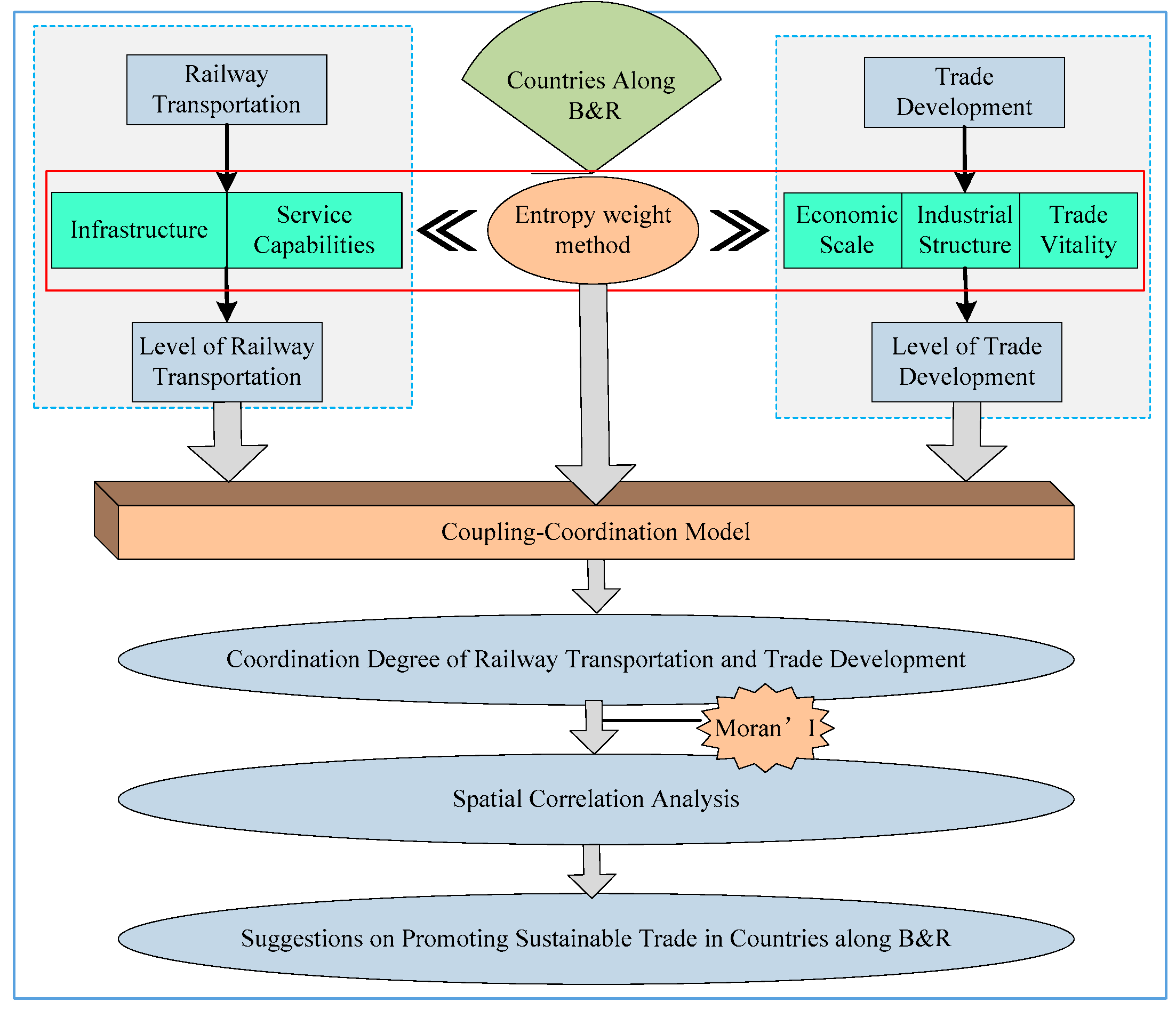
When compared with previous studies, we produced some improvements. First, we analyzed the interaction between railway transportation and trade and then studied the important role of railway in the sustainable development of trade. Railway transportation evaluation indicators from the aspects of railway transportation infrastructure and service capacity were constructed. The scale of trade, industrial structure, and trade vitality were used to construct trade evaluation indicators. Second, when combined with a geographic information system (ArcGIS, 12.6, Esri, Redlands, America), the spatial evolution of the coordination degree between railway transportation and trade development was demonstrated. Relevant measures were proposed to promote the coordinated development of railway transportation and trade, achieve the sustainable development of trade, support the implementation of the Belt and Road, and provide a theoretical basis for reshaping the time and space patterns and patterns of countries along the B&R. Simultaneously, we provide a theoretical basis for the subsequent theoretical study of sustainable trade from the spatial perspective. Figure 1 presents our research framework.
The rest of the paper is organized as follows. Section 2 introduces the evaluation index of railway transportation, trade development, and the coupling-coordination measurement model of the two; Section 3 presents the calculation result of the level of railway transportation (LRT), the level of trade development (LTD), the coordination degree of the railway transportation and trade development (CRT), the spatial situation analysis of the coordination degree, and the spatial effect analysis. Section 4 summarizes the full text and then provides corresponding recommendations.

2. Methods, Indicators and Data

2.1. Methods

2.1.1. Coordination Degree

Coordination degree refers to the degree to which two interacting systems simultaneously develop. The higher the synergy level, the higher the synchronicity of the development of the two systems and the more coordinated their development. A lower synergy level indicates that they are not synchronized. Synergistic effects occur when the two systems work together. The synergistic effect enhances the two systems, producing a larger overall effect [47]. For the countries along the Belt and Road, the coordinated development of railway transportation and trade and their synergistic effects will achieve the sustainable development of trade along the B&R. A coupling-coordination model can measure the synergy level. Coupling degree reflects the correlation degree among systems. The more linkages among systems there are, the larger the correlation degree is. There are many interactions among the railway transportation and trade development. However, in some cases, it does not reflect the synergies effect among the systems. The coordination degree is used to reflect the synergies among systems [48]. Therefore, this study constructs a coupling-coordination model to evaluate the synergy level. The calculation steps are as follows:
Step 1: Calculate the degree of interaction between the two subsystems, i.e., the degree of coupling, and the calculation formula is as follows:
C C R T = { L T D i × L R T i ( α L T D i + β L R T i ) θ } 1 θ
where α and β are the weights for the contribution of railway transportation and trade development to coupling degree, respectively, and α + β = 1 , while considering that railway transportation can promote the development of trade and trade can also instigate the further development of railway transportation. Therefore, the interactions between railway transportation and trade cannot be ignored. Sun et al. [49] was referred to, so we set α = β = 0.5 , θ is the number of subsystems. As we choose the two systems of railways transportation and trade development in this study, θ = 2. The i represents the ith country. The C C R T represents the coupling degree of railway transportation and trade, 0 C C R T 1 . A greater value of C C R T indicates that there is benign development between the level of railway transportation and trade, so railway transportation can achieve more coordinated development with trade development. L T D i and L R T i indicate the levels of trade development and railway transportation, respectively. These are obtained by dimensionless processing, standardization processing, and the weight calculation of the entropy weight method for indicators.
According to the calculation results of the coupling degree, the coupling degrees were divided into six levels for judgment [50]. Table 1 shows the division criteria.
Step 2: Calculate the synergy level of the two systems using Equation (2) based on the calculation results of the coupling degree.
C R T = C C R T × M
M = α L T D i + β L R T i
where CRT is the coordination degree, C C R T is the coupling degree, and M is the comprehensive reconciliation index for the level of railway transportation and the level of trade development.
According to Cui [51], the coordination degree can be divided into four levels. Table 2 outlines the specific classification.

2.1.2. Spatial Autocorrelation Analysis

The purpose of spatial autocorrelation analysis is to describe the spatial distribution characteristics of the CRT and judge the interdependence of the CRT. Moran’s I is one of the most common indicators used for examining spatial autocorrelation [52,53].
Step 1: Moran’s index calculation
The spatial effect of CRT is expressed as I C R T using the Moran’s index, and its calculation formula is as follows:
I C R T = n i j w i j ( C R T i C R T ¯ ) ( C R T j C R T ¯ ) ( i j w i j ) i ( C R T i C R T ¯ ) 2 ( i , j = 1 , 2 , , 40 )
where C R T ¯ represents the average of the CRT, n is the number of countries along the B&R, and wij is the element of the spatial weight matrix of each country along the B&R. Among them, the adjacency rule and the distance rule usually determine the spatial weight matrix [54]. We selected the adjacency rules shown as Equation (5). The I C R T takes values in (−1,1). When I C R T < 0 , there is a negative spatial correlation in the space, meaning that the space distribution characteristics are high CRTs and low CRTs aggregating, The closer the value is to −1, the more obvious the aggregation phenomenon. When I C R T > 0 , there is a positive spatial correlation in the space, meaning that the space distribution characteristics are an aggregation of high (low) CRTs with high (low) CRTs. When I C R T = 0 , there is no spatial correlation, this situation is called randomly distributed in space.
w i j = { 1 ,   region   i   and   region   j   are   adjacent 0 ,   region   i   and   region   j   are   not   adjacent  
Step 2: Significance test
The significance of the spatial autocorrelation can be verified by the Z value [55]. Its calculation formula is as follows:
Z C R T = I C R T E ( I C R T ) V ( I C R T )
where E ( I C R T ) = 1 / ( n 1 ) and V ( I C R T ) = E ( I C R T 2 ) E ( I C R T ) 2 . Table 3 shows the corresponding relationships between the Z value, the p value, and the significance level. We used GeoDa (The GeoDa Center for Geospatial Analysis and Computation, Chicago, America) software to test for significance.

2.2. Indicators and Data

We constructed the evaluation index for railway transportation from infrastructure and service capacity and then constructed the evaluation index for trade from the aspects of economic scale, industrial structure, and trade vitality, as a country’s railway transportation is usually related to the country’s land area and population, in order to objectively reflect the level of railway transportation in various countries along the B&R. When constructing the index system for railway transportation, we considered the four indicators: per capita railway mileage, railway network density, per capita railway transportation turnover, and railway transportation intensity. Table 4 shows the 13 indicators that were selected for this paper.
Currently, the B&R initiative includes 65 countries, including Syria, Palestine, the United Arab Emirates, Lebanon, Egypt, Bahrain, Kuwait, Lebanon, Cyprus, Yemen, Montenegro, Oman, Jordan, Qatar, Singapore, Laos, Cambodia, Myanmar, Sri Lanka, Indonesia, Philippines, Maldives, Nepal, Brunei, and Serbia. Among those 25 countries, some have little land area and almost no railway transportation. Some countries have been constantly at war, so their statistics are missing considerable information. Therefore, the paper used the other 40 countries of the Belt and Road as the research object, which are Albania (ALB), Azerbaijan (AZE), Estonia (EST), Pakistan (PAK), Belarus (BLR), Bulgaria (BGR), Poland (POL), Bosnia and Herzegovina (BIH), Russian Federation (RUS), Georgia (GEO), Kazakhstan (KAZ), Kyrgyz Republic (KGZ), Czech Republic (CZE), Croatia (HRV), Latvia (LVA), Lithuania (LTU), Romania (ROM), Malaysia (MYS), Macedonia (MKD), Mongolia (MNG), Bangladesh (BGD), Moldova (MDA), Saudi Arabia (SAU), Slovak Republic (SVK), Slovenia (SVK), Tajikistan (TJK), Thailand (THA), Turkey (TUR), Turkmenistan (TKM), Ukraine (UKR), Uzbekistan (UZB), Greece (GRC), Hungary (HUN), Armenia (ARM), Iraq (IRQ), Iran (IRN), Israel (ISR), India (IND), Vietnam (VNM), and China (CHN). The data of the 13 indicators were obtained from the official statistics of the World Bank [56].

3. Results and Discussion

3.1. Level of Railway Transportation and Trade Development

Figure 2 shows the average level of the railway transportation and trade development in 40 countries along the B&R during the period of 2006 to 2016.
The average level of railway transportation (LRT) for all countries along the B&R from 2006 to 2016 is 0.204. As shown in Figure 2a, 42.5% of the countries had the high LRTs of more than 0.204, while 57.5% of the countries had the low LRTs of less than 0.204. LRTs along the B&R had the spatial distribution characteristics of “low on the south and high on the north”. This means that countries with high LRTs are probably distributed in Southeast Asia, Central Asia, and West Asia; meanwhile, the countries with low LRTs are distributed in Central and Eastern Europe and East Asia.
The average level of trade development (LTD) for all countries along the B&R from 2006 to 2016 is 0.224. As shown in Figure 2b, 45.0% of the countries had the high LTDs of more than 0.224, while 55.0% of the countries had the low LTDs less than 0.224. LTDs along the B&R had the spatial distribution characteristics of “low middle and high on both sides”. This means that most of the countries in East Asian economic circle at the eastern end and the European economic circle at the western end had relatively high LTDs, while countries in the vast inland and South Asia in the middle had low LTDs.
Figure 3 shows the average level of railway transportation and trade development of 40 countries from 2006–2016. The average LRTs is lower than average LTDs, indicating that the development of railways transportation lagged behind trade development along the B&R during the 11 years. Both the average LRTs and the average LTDs had the same downward trend. The average LRTs decreased from 0.212 to 0.186, with a 12.16%-fold decrease, which may be related to the vigorous development of other modes of transport. While the average LTDs decreased from 0.247 to 0.182 with a 26.32%-fold decrease, which might be related to a significant reduction in foreign direct investment in many countries.
Figure 4 shows coefficient variation (CV) between the level of railway transportation and trade development. During the 11 years, the CV of LRT is relatively stable, while the CV of LTD has a slowly growing tendency. It indicates that the developmental difference of economy and trade among countries along B&R is gradually increasing. The CV of LRT is nearly twice that of LTD, which means that the development difference of LRT is more significant. This may be related to the geographical characteristics and the economic structure of these countries, hindering the railways to become the most economical means of transportation in many countries.

3.2. Coupling-Coordination Results

Table 5 shows the calculation results of the coupling degree of the LRT and LTD along the B&R. The results showed that the average degree of coupling between the LRT and LTD in the countries along the B&R was significantly higher than 0.7, indicating that railway transportation and trade are mutually coupled. Railway transportation had many correlations with trade. As shown in Table 5, SVK and SVN had the higher coupling degree, because SVK and SVN had a high LRT and a high LTD, which makes it possible for railway transportation have more interaction with trade and economy. The coupling degrees of KGZ, IRQ, and SAU were lower, among which SAU was the lowest because SAU had a lower LRT, but a high LTD and the development of railway transportation in the country was backward and inconsistent with trade. When combined with the coupling degree classification in Table 1, the classifications of 40 countries are shown in Table 6. 17.5% of countries were in the low level coupling stage and 25% of countries were in the run-in phase where that the role of railway transportation in trade was becoming increasingly obvious. A total of 57.5% of the countries had a high level of coupling, which indicates that railways transportation had strong interaction with trade in most countries along B&R.
Table 7 shows the results of the coordination degree of railway transportation and trade development (CRT) along the B&R. The results showed that the average degree of coordination between railway transportation and trade in the countries along the B&R was lower than 0.4, indicating that railway transportation and trade did not have a coordinated development. The CV of CRTs among the countries from 2006 to 2016 is in the interval of 0.421–0.462 and it had a decreased tendency, which indicates that the differences in 40 countries from 2006 to 2016 were smaller. The CRTs of countries along the B&R have a tendency of balanced development. As shown in Table 7, the coordination degrees in KGZ, IRQ, and SAU were lower, mainly because that the trade development is too dependent on oil transportation through shipping. KGZ and IRQ are because trade development is mainly based on road transportation. The coordination degree in SVK was the highest, because SVK is a landlocked country and industry accounts for a relatively high proportion of its GDP and it was mainly based on railways. This makes the railways and trade have a synchronous development trend and shows a higher coordination degree. Combined with Table 2, the coordination degree classification is shown on Table 8, and the results showed that 42.5% of the countries along the B&R were classified as low coordination, 32.5% were moderate coordination, and only 25% were high coordination. The coordinated development of railways and trade in the countries along the B&R is extremely uneven.
Figure 5 illustrates the spatial evolution of the coordination degree. As seen in Figure 5, the changes in the coordination degree between countries along the B&R in 2006 and 2013 were relatively small. KAZ, RUS, and many countries in Central and Eastern Europe had higher CRTs. Countries in Central Asia mostly had lower CRTs. From 2006 to 2013, China’s CRT increased remarkably, which showed that the degree of simultaneous development of railway transportation and trade is increasing. In 2016, significant changes in the CRT occurred between countries along the B&R, with the obvious spatial distribution characteristics of “low in the east and middle but high in the west”, indicating that the CRT in the countries in the East Asian economic circle and the vast inland area was lower, while some countries in the European economic circle were higher. Among them, KAZ, RUS, CHN, and IND experienced significant decline in their coordination degree in 2016. The main reason for this finding is that countries along the B&R have strengthened the links in trade with the steady advancement of the B&R initiative after 2013. However, due to the lag in railway transportation construction and development, the level of railway transportation has seriously lagged behind the level of trade development, which has intensified the inconsistency of railway transportation and trade.
Figure 6 shows the characteristics of coupling-coordination distribution for the LRT and LTD in the countries along the B&R. If a country has a high degree of coupling and high degree of coordination, it means that there is a strong interaction between the railway and the trade, and the two play the synergistic effect and achieve sustainable trade. A country with a high degree of coupling but low degree of coordination has good basic conditions and the potential for achieving sustainable trade, and it should fully play the role of railways in trade. If a country has a low degree of coupling and a low degree of coordination, then it has limited interaction between railways and trade. As shown in Figure 6, THA, VNM, MYS, SAU, TJK, KGZ, and IRQ had a low degree of coupling and a low degree of coordination, which indicated that railway transportation in THA, VNM, MYS, SAU, TJK, KGZ, and IRQ played a weak role in trade. Among them, THA, VNM, MYS, and SAU are close to the sea, and their trade development mainly depends on shipping. Due to the backwardness of TJK, KGZ, and IRQ, the development of their economies and trade mainly relies on road transportation.
The run-in phase in the coupling model refers to the phase in which the two systems of railway transportation and trade adapt to each other, where the interaction between railway transportation and trade is continuously strengthened. The two systems in the run-in phase usually shift from a lower interaction degree to a higher degree. As shown in Figure 6, 25% of countries were in the run-in phase. Among them, the CRTs in TUR, ALB, IRN, BIH, and GRC were low. According to the original index system, TUR, BIH, and GRC are insufficient in railway transportation intensity. Due to the low density of railway networks in ALB and IRN, the development of railway transportation and trade has been uncoordinated. The CRTs in UKR and KAZ were moderate, because UKR has a low direct external gross domestic product (GDP) and trade vitality on the economic scale and KAZ has a low import of goods and services. The CRTs in RUS and CHN were high, because they both have sound railway infrastructures and large transportation service capacity, so railway transportation can meet the requirements for trade.
In countries with a high coupling degree, MKD, ARM, UZB, BGD, and PAK had a lower CRT. Among them, MKD and BGD had a low railway transportation intensity and low railway mileage per capita. ARM, UZB, and PAK had a low overall effect on the LRT and LTD. IND, BGR, POL, MNG, TKM, ROM, GEO, AZE, MDA, and ISR had moderate CRTs. IND was among them, because it has a low net inflow of foreign direct investment in trade, low import and export of goods, low import of goods and services, and a low per capita GDP on the economic scale. BGR, AZE, MDA, ROM, and GEO had low railway operation service capacity. ISR had lower railway transportation turnover per capita. TKM had a lower tertiary industry and POL had a lower net foreign direct investment in trade vitality. MNG’s railway density was low, which led to the moderate coordination degree. CZE, SVK, HUN, SVN, LTU, EST, and BLR had high coordination degrees, which indicated that there was a strong interaction between railway transportation and trade and had achieved coordinated development. Therefore, railway transportation could support the sustainable development of trade and play a synergistic effect.

3.3. Spatial Autocorrelation Analysis

Figure 5 shows that there was a spatial aggregation of the CRT. In order to further study the spatial relationships of the CRTs along the B&R, we used Equations (4)–(6) to measure the Moran’s index of CRTs from 2006 to 2016. Table 9 shows the results. Figure 6 is a map of the Moran’s index between 2006 and 2016, reflecting the changing trends in spatial correlation.
The results showed that the global Moran’s indexes of CRTs from 2006 to 2016 were greater than 0 and greater than E[I], which passed the 95% confidence level significance test in 2006–2015, and the Z value was greater than 1.96. This demonstrated the significant positive correlation between the CRTs in space over the 10 years. The CRTs in countries that were along the B&R remained consistent for the past 11 years, which means that countries with high CRTs are surrounded by countries with high CRTs, and countries with low CRTs are surrounded by countries with low CRTs. The global Moran’s index was stable and then declined from 2006 to 2009, which means that the CRTs had begun to spread evenly among countries. However, during 2013–2016, there was a clear upward trend, indicating that the characteristics of the CRTs space aggregation among countries became increasingly obvious. Matthew Effect is coined by Robert K. Merton and it is often summarized by the adage “the richer get richer and the poor get poor” [57]. Existing research on the Matthew Effect considers that this dynamic effect can alter information flow and the distribution of rewards in the ways that lead to cumulating advantages for high status actors [58]. Based on the definition of Matthew effect and existing research, we find that CRTs in countries along the B&R have the Matthew effect in space, which means that there is the agglomeration trend of countries with high CRTs or the agglomeration trend of countries with low CRTs. The Moran’s I during 2006–2016 had an upward trend, as shown in the red line in Figure 6, which means that the agglomeration trend of countries with high CRTs is strengthened, likewise the agglomeration trend of the countries with low CRTs become stronger. That is, the Matthew effect was more significant over time along the B&R. The average of global Moran’ I is 0.440, and I of CRTs after 2013 is higher than the average, which means that the imbalance of CRTs has intensified after 2013 when the B&R initiative was put forward.
The global Moran’s I index represents the mean value of the local Moran’s I index, and makes it impossible to determine whether there is a negative spatial autocorrelation. Therefore, to further analyze the local spatial autocorrelation of CRTs in the countries along B&R, we mapped the countries onto a Moran scatter plot for the years of 2006, 2013, and 2016, as shown in Figure 7. Table 10 shows the corresponding permutation test results.
As shown on Figure 8, the first quadrant on the Moran scatter plot represents a country with a high CRT with its surrounding countries having high CRTs (HH); the second quadrant represents a country with a low CRT with its surrounding countries having a high CRT; the third quadrant represents a low CRT with its surrounding countries having a low CRT; and, the fourth quadrant represents a high CRT with its surrounding countries having a low CRT. During the study period, about 37.5% of the countries were in the first quadrant and 27.5% of the countries were in the third quadrant, which indicates a positive spatial correlation of CRT in most countries. Countries with higher CRTs and countries with lower CRTs showed obvious aggregation, respectively. However, in the studied years, some of the countries were found in the second and fourth quadrant, which means that there are still negative spatial autocorrelations in some countries.
Figure 8 shows that during the three years studied, the spatial position of the CRTs varied slightly, which means that the Belt and Road initiative has not brought about major changes to the CRTs. Countries in Central and Eastern Europe, including RUS, were mainly distributed in the first quadrant, and the railway transportation has developed more in coordination with trade in these countries. However, it has not yet formed a radiation effect on the adjacent countries in West Asia, like the less developed ALB and BGR, which is due to the lag of facility construction. However, CHN, IND, and KAZ were always in the fourth quadrant and had a spatial distribution of HL, which indicated that countries adjacent to these countries had not fully utilized the space spillover effect to achieve the coordinated development of domestic railway transportation and trade. From 2006 to 2013, the significant increase in the spatial position of VNM and BGD indicated that the difference in CRTs between them and their surrounding countries was increasing. From 2013 to 2016, the decline in the relative positions of EST and RUS indicated that they could make full use of the development opportunities of the B&R and they achieved the coordinated development of railway transportation and trade, which closed the gap in the CRTs between them and their surrounding countries.
Table 10 shows the values of the local Moran’s index, which reflects the spatial correlation of CRTs in countries along the B&R. When the value is greater than 0, the country has the same coordination degree distribution status as its neighboring countries. When the value is less than 0, the country’s CRT is significantly different from its surrounding countries. The results showed that the CRTs in the countries that passed the significant test were greater than 0, which means those countries distributed in the same state with their surrounding countries. Among them, the aggregation states of BGR, EST, HUN, SVK, THA, UKR, and UZB appeared to be weakened at first and then strengthened, which indicated that the distribution of CRTs in these countries and their surrounding countries is relatively uniform and the aggregation characteristics were weakened. However, with the development of railway transportation and the steady advancement of trade, the aggregation characteristics of CRTs in these countries and their surrounding countries had increased. BLR, LTU, LVA, and SAU were first strengthened and then weakened, which indicated that there were stronger spatial aggregation characteristics in these countries and their surrounding countries in 2013. However, CRTs tend to be randomly distributed among these countries in 2016, which is mainly due to the balanced development of railways and trade in these countries. The aggregation states of CZE and SVN were always strong. The aggregation states of IRN, IRQ, POL, and RUS were always weak. Among them, the decrease in RUS was more significant (about 89.01%), showing that the difference in the CRT between RUS and its surrounding countries was decreasing, and that the CRT tended to be more evenly distributed.
Figure 8 shows that the CRTs had an overall positive spatial correlation in the countries along the B&R. In order to display better the spatial relationship between one country’s CRT and the surrounding countries’ CRT, we used local spatial autocorrelation to study the local Moran’s index of the CRTs and used GeoDa to draw the LISA (Local Indicators of Spatial Association) aggregation maps of CRTs for 2006, 2013, and 2016, as shown in Figure 9. The representation of the marked color in the figure passed the test at a significance level of 95%. The results showed that the spatial correlation of the CRTs along the B&R was mainly determined by high-high and low-low aggregation.
There were 11 countries in Central and Eastern Europe, where the CRTs had a strong positive spatial correlation. IRQ and SAU had a negative spatial correlation. Among them, RUS had a positive spatial correlation in 2013, but there was no obvious spatial correlation in 2016. However, UZB and TJK had a negative spatial correlation since 2013. The results also showed that railway transportation and trade along the B&R had not yet achieved coordinated development, and many countries had not yet shown significant aggregation characteristics. Countries along the B&R should continue to enhance the role of railway transportation in trade, achieve the synergistic development of railway transportation and trade, and achieve the sustainable development of trade along the B&R.

4. Conclusions and Suggestions

In this study, we constructed an evaluation index system for railway transportation (railway infrastructure and operational service capability) and trade development (economic scale, industrial structure, and trade vitality). Based on the entropy method, the LRT and LTD in the countries along the B&R were calculated. When combined with the coupling-coordination model, the coordination degree was calculated and its spatial evolution was further studied.
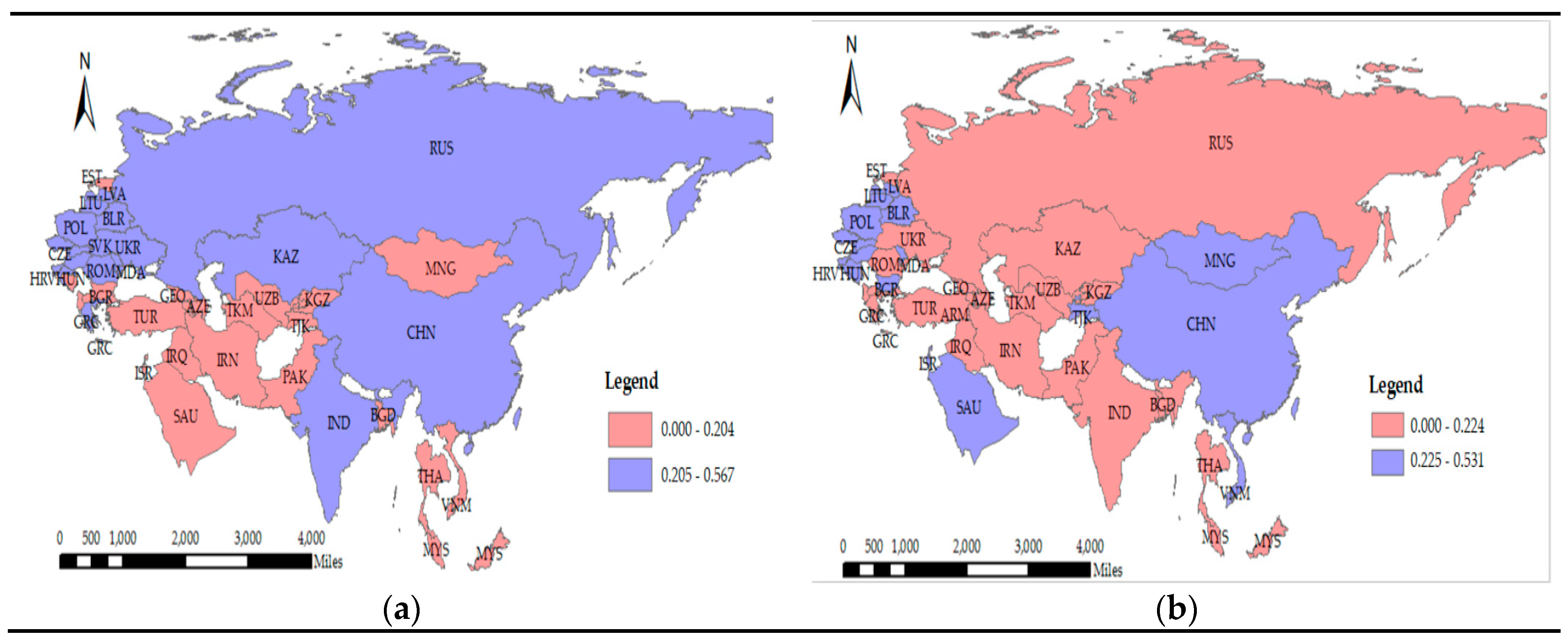
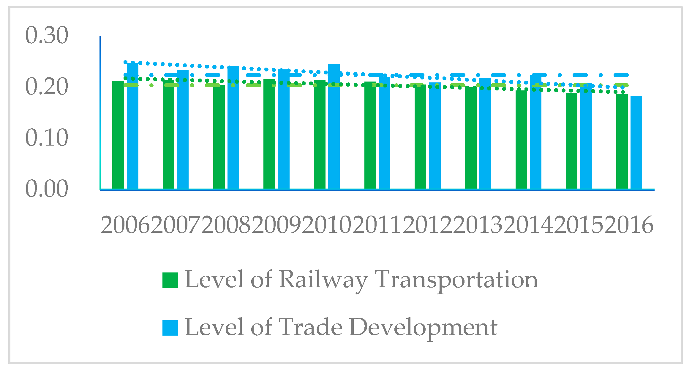
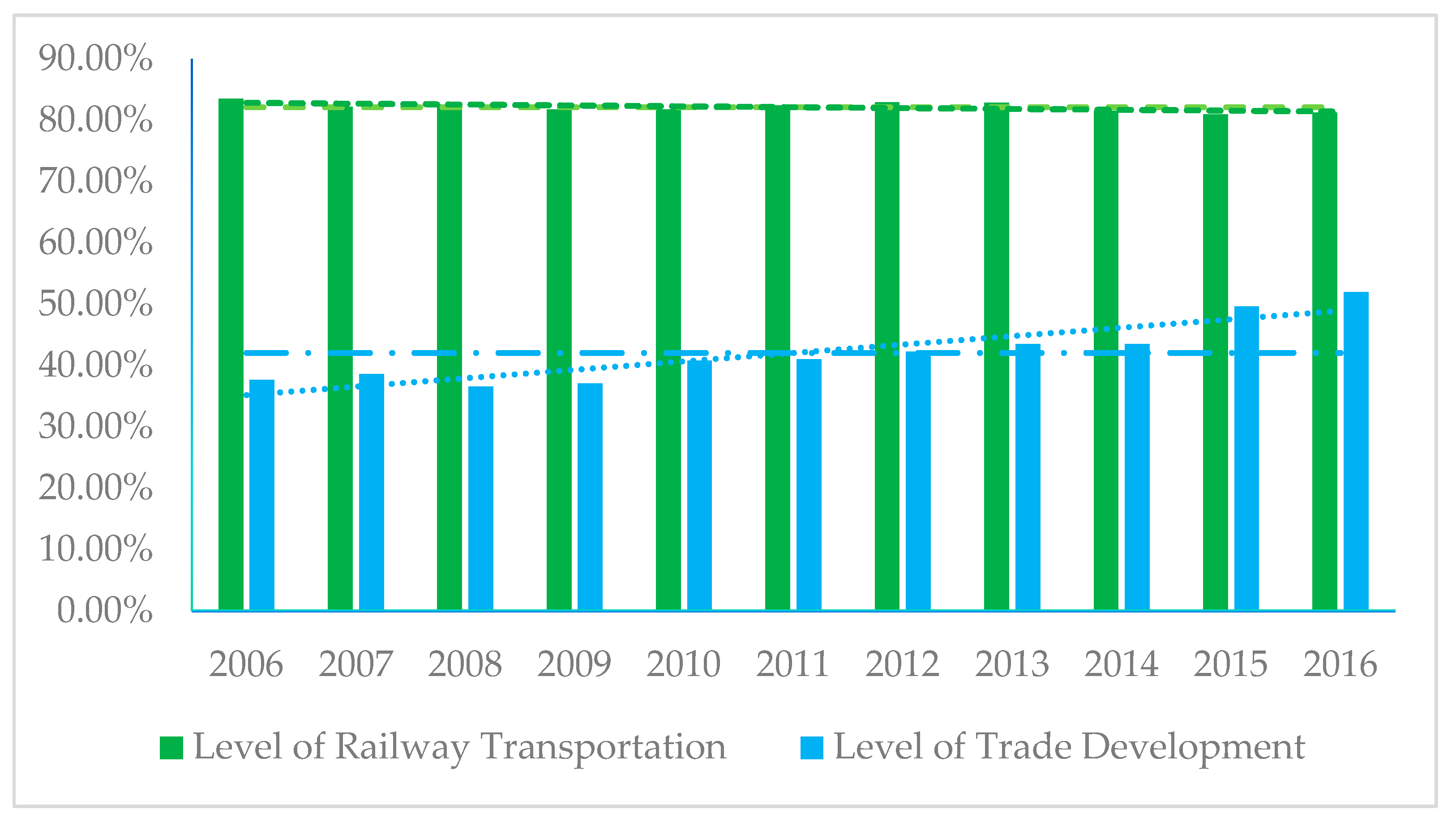
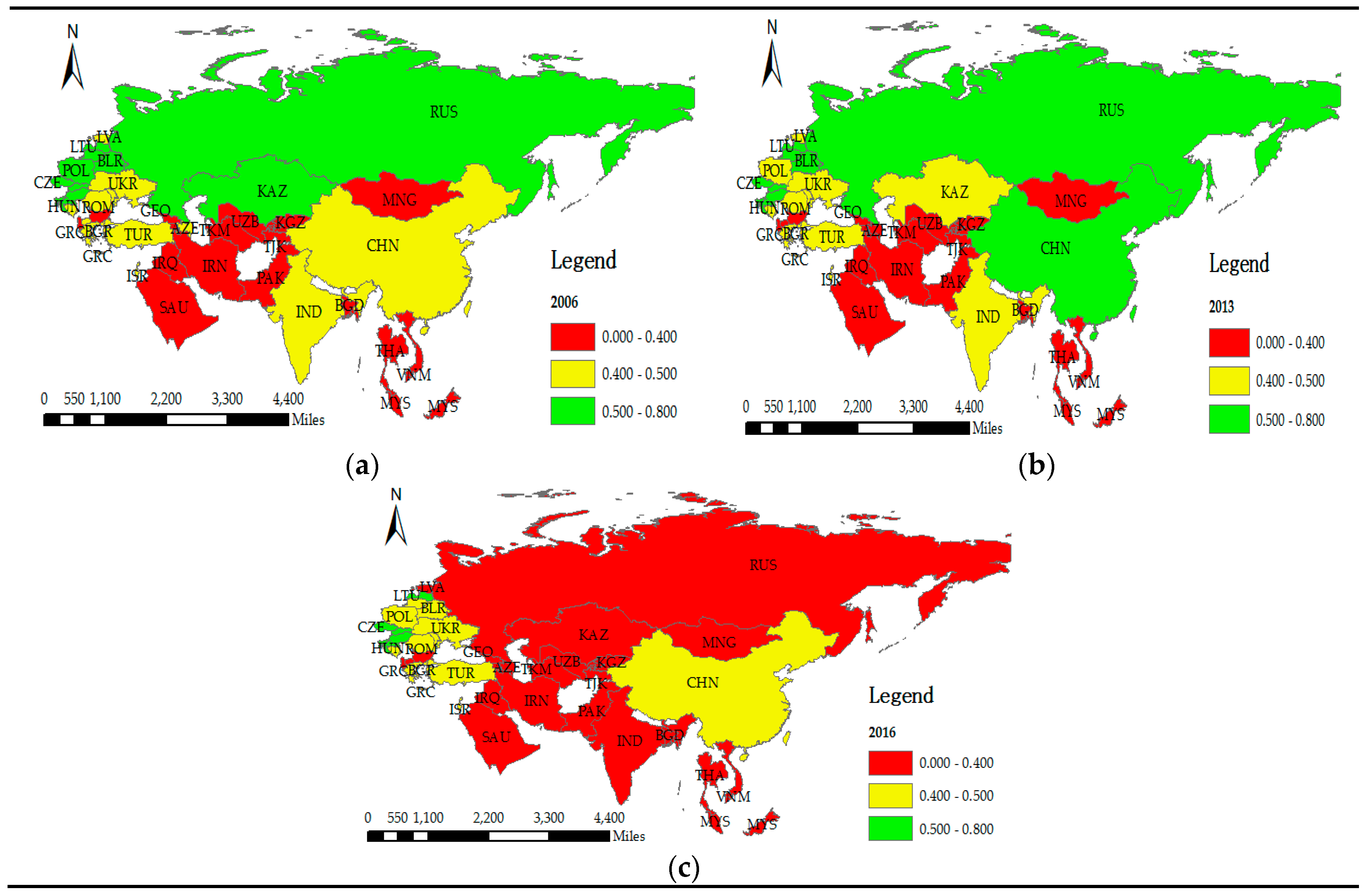
As seen from the calculated results of the LRT and LTD, the LRTs among the B&R countries were unevenly distributed, and they had a spatial distribution characteristic of “low on the south and high on the north”, meaning that countries with high LRTs are probably distributed in Southeast Asia, Central Asia, and West Asia, meanwhile, countries with low LRTs are distributed in Central and Eastern Europe and East Asia. About 45.0% of the countries’ LRTs were high and 55.0% of the countries’ LRTs were relatively low. The average LRTs and the average LTDs had the same downward trend, indicating that there was no significant change in the development of railway transportation and trade in various countries along the B&R after the proposal of the Belt and Road Initiative. Considerable unbalance still exists in the LRTs and LTDs among the countries along the B&R.
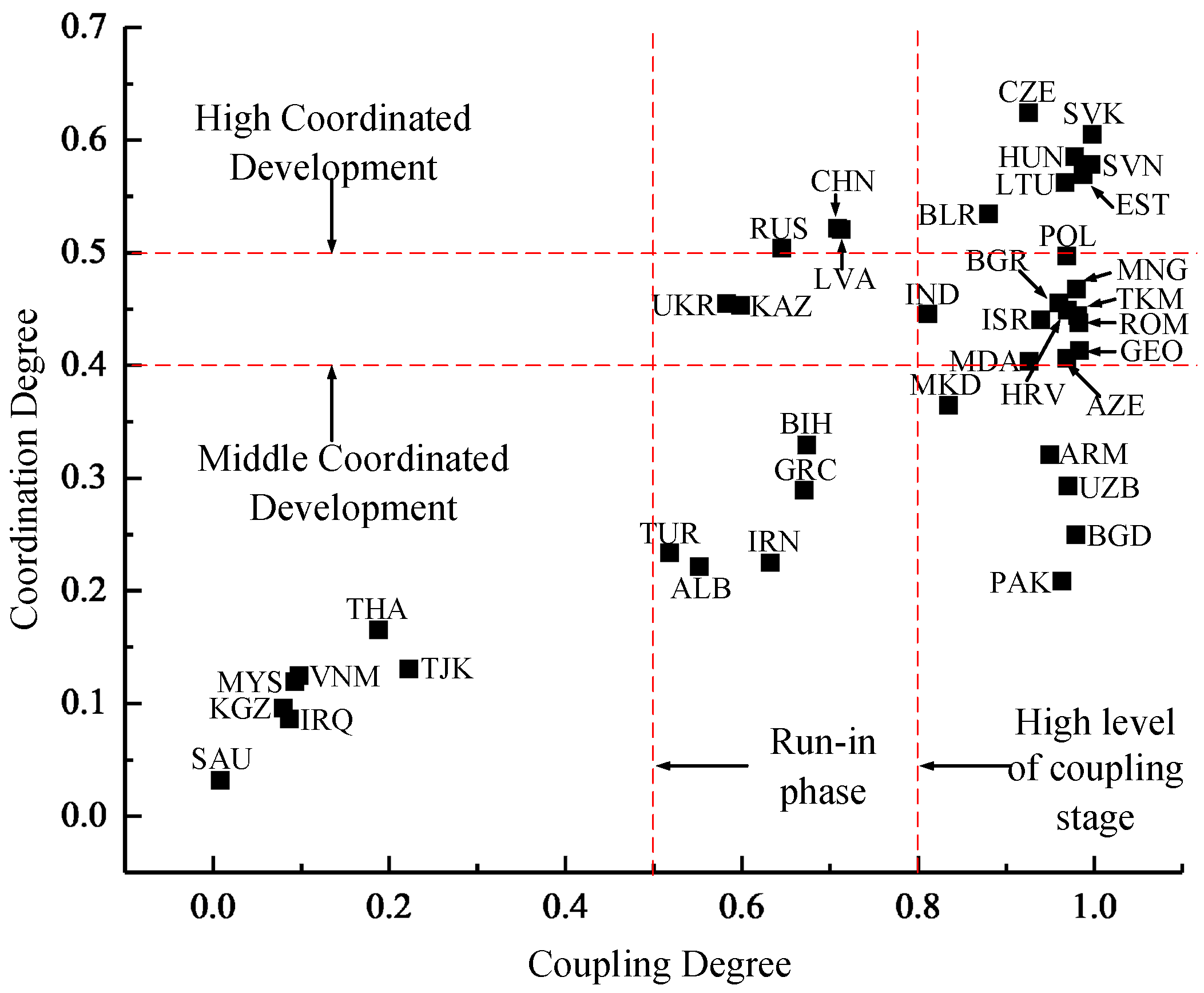
As seen from the calculated results of the coupling degree, the average coupling degree between the LRT and LTD in the countries along the B&R was between 0.717 and 0.737, which means that railway transportation along the B&R had many correlations with trade. Among them, 17.5% of countries were in the low level coupling stage, 25% of countries were in the Run-in phase, and 57.5% of the countries had a high level of coupling. The results of the coordination degree showed that only 25% of countries in Central and Eastern Europe had achieved highly coordinated development of railway transportation and trade. Most of the countries in Central and Eastern Europe are small in area and railway transportation and do not exert their own advantages. Southeast Asian countries and some Central and Eastern European countries had lower CRTs as railways are not the main mode of transportation in trade, because they have natural harbors that are used instead. For these countries, they can increase railway infrastructure construction in the future and improve the level of railway operations. These countries should also make full use of the advantages of railway transportation and maritime transportation to realize sustainable trade development. The CRTs of the countries in Central and West Asia were low, which is mainly because these countries have relatively low economic development. They should increase railway infrastructure construction in the future and seize the opportunity that is provided by the Belt and Road initiative to achieve the coordinated development of railway transportation and trade.
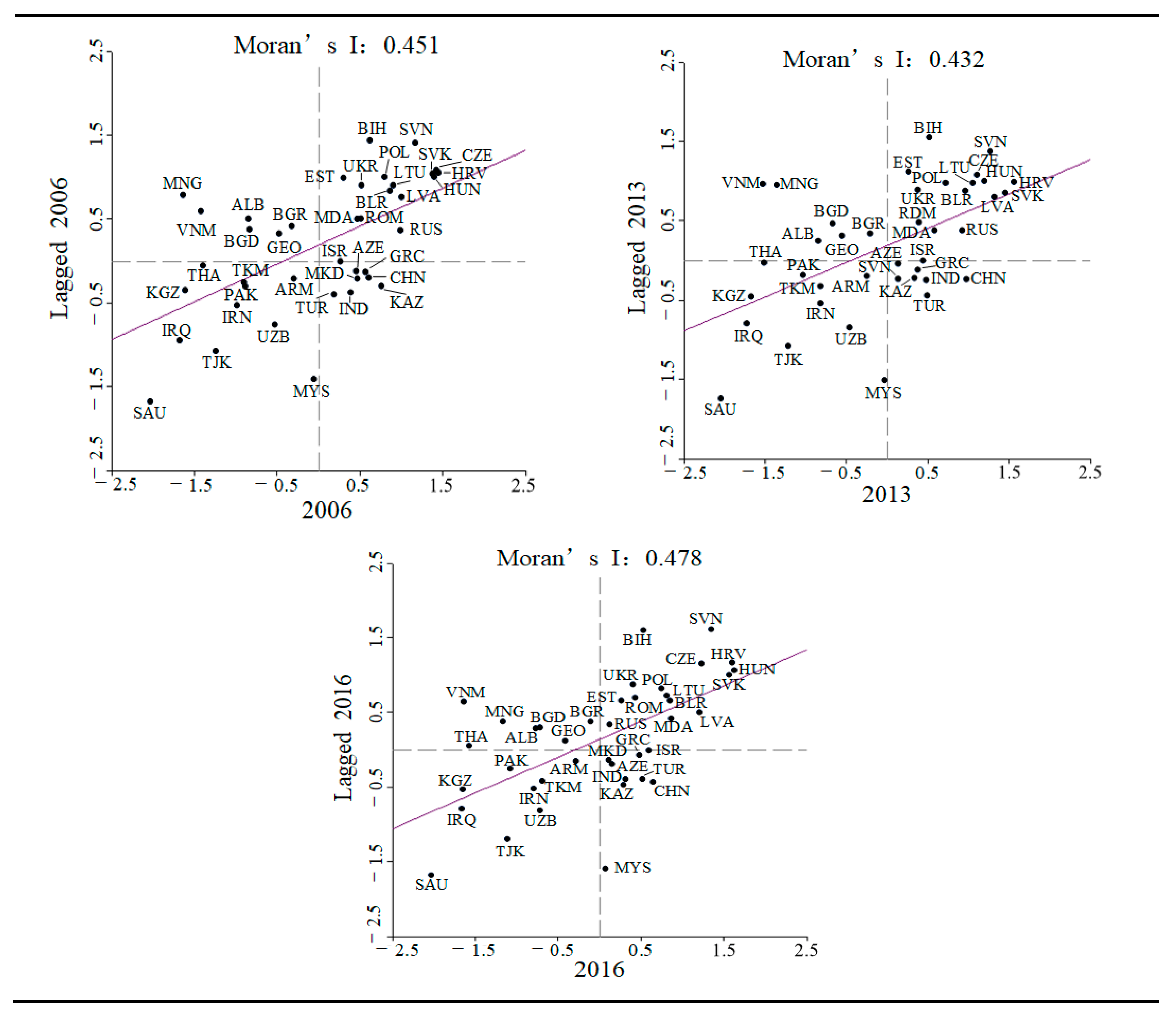
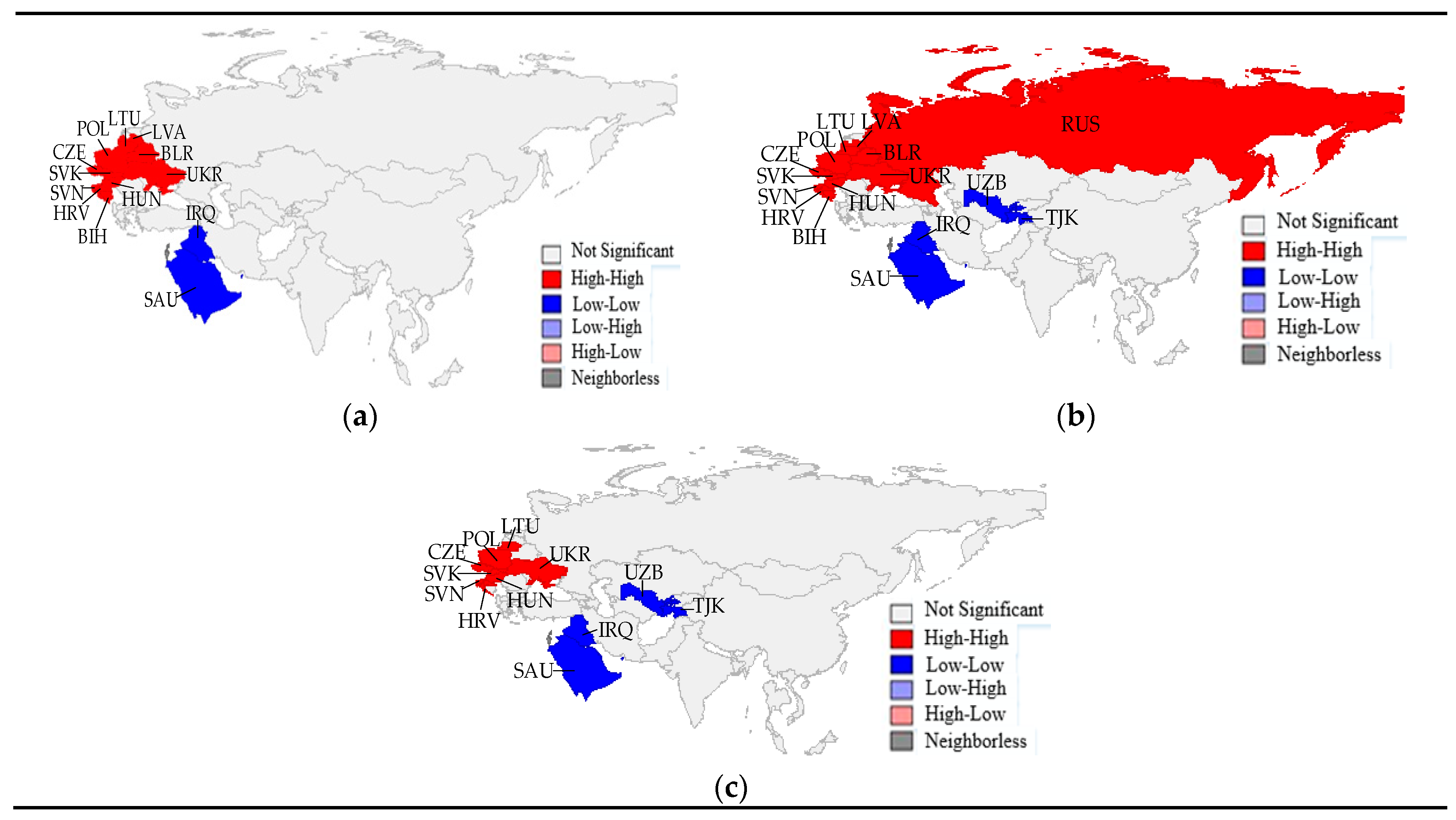
The spatial correlation analysis showed that there was a significant positive spatial correlation between the CRTs, that is, there were high-high aggregation and low–low aggregation in the CRTs along the B&R. The CRTs along the B&R had obvious Matthew effects in space, and the Matthew effect is more significant over time along the B&R. The CRTs in space distributed unevenly and countries along the B&R urgently need to achieve the coordinated development of railway transportation. At the same time, countries along the B&R should play the spatial and radiative effects of high-coordination countries, take advantage of the railway transportation of the countries along B&R, realize the effective flow of goods between the countries, and form sustainable development that is based on the sharing of railway resources.
Our study also has some limitations. The first potential defect may exist in the coupling analysis process of two related variables of railway infrastructure and trade volume. Obviously, there is a clear correlation between the level of railway transportation and the trade volume. However, the changes in railway infrastructure have been relatively slow, while the trade volume has fluctuated greatly due to numerous exogenous effects. Therefore, the robustness of the results of the coupling analysis of the two variables may be affected. The study is also trying to eliminate this problem. On the one hand, we have chosen the indicator of 11 years to measure the coupling and coordination relationship between the annual railway transportation and trade development level. On the other hand, the railway transportation level includes not only the indicators of railway infrastructure, but also the indicators of transportation volume and other factors that are greatly affected by exogenous variables. Secondly, for the limitation of data availability in the whole regions of B&R we mainly constructed the evaluation index system from the perspectives of economic scale, industrial structure, trade vitality, infrastructure and service capabilities for the sustainable development of trade. However, some indexes that are also important to sustainable trade, such as ecological indicators, were not included in this study. With the gradual improvement in relevant statistical data of countries along the B&R, future study will enrich the indicator system and analyze the coordinated development of railway transportation and trade in multiple dimensions.

Author Contributions

Q.S. established the research framework; X.W. and F.M. jointly established the research model; Y.H. and Q.C. collected the data and carried out the result calculations; Q.S. provided the data acquisition channel; and Q.S. and X.W. analyzed the results and wrote the paper together.

Funding

This study was financially supported by the National Social Science Foundation of China (grant number 17BJY139).

Conflicts of Interest

The authors declare no conflict of interest.

References

  1. Lee, T.H.; Jan, F.H. Can community-based tourism contribute to sustainable development? Evidence from residents’ perceptions of the sustainability. Tour. Manag. 2019, 70, 368–380. [Google Scholar] [CrossRef]
  2. Sakib, N.; Appiotti, F.; Magni, F.; Maragno, D.; Innocenti, A.; Gissi, E.; Musco, F. Addressing the Passenger Transport and Accessibility Enablers for Sustainable Development. Sustainability 2018, 10, 903. [Google Scholar] [CrossRef]
  3. IPCC. Climate Change 2014: Synthesis Report; Contribution of Working Groups I, II and III to the Fifth Assessment Report of the Intergovernmental Panel on Climate Change; Pachauri, R.K., Meyer, L.A., Eds.; IPCC: Geneva, Switzerland, 2014; 151p. [Google Scholar]
  4. IEA. CO2 Emissions from Fuel Combustion; International Energy Agency: Paris, France, 2014. [Google Scholar]
  5. Network of the Central People’s Government of the People’s Republic of China. Target lock! “Three-Year Action Plan to Win the Blue Sky Defence War” Is about to Be Implemented. Available online: http://www.gov.cn/zhengce/2018-06/20/content_5299968.htm (accessed on 31 May 2018).
  6. Mulley, C.; Hensher, D.A. Is rail cleaner and greener than bus? Transp. Res. Part D Transp. Environ. 2017, 51, 14–28. [Google Scholar] [CrossRef]
  7. Dobbin, F. Forging Industrial Policy: The United States, Britain and France in the Rail-Way Age; Cambridge University Press: London, UK, 1997. [Google Scholar]
  8. Yu, H.; Dong, S.; Li, Y.; Li, Z.; Shi, G.; Li, F.; Li, F.; Chang, Y. China’s Geopolitical Strategy of the Belt and Road Initiative Based on Theory of Externality. Bull. Chin. Acad. Sci. 2016, 31, 697–706. [Google Scholar]
  9. Liu, H.; Wuzhati, Y.; Wang, C. Impacts of the Belt and Road Initiative on the spatial pattern of territory development in China. Prog. Geogr. 2015, 34, 2080–2087. [Google Scholar]
  10. China Belt and Road Network. CHINA RAILWAY Express. Available online: https://www.yidaiyilu.gov.cn/zchj/rcjd/60645.htm (accessed on 23 November 2018).
  11. Martin, P.; Rogers, C.A. Industrial location and public infrastructure. J. Int. Econ. 1995, 39, 335–351. [Google Scholar] [CrossRef]
  12. Gillen, D.W. Public Capital, Productivity, and the Linkages to the Economy: Transportation Infrastructure. Policy Study 2001, 34, 1–31. [Google Scholar]
  13. Bonfatti, R.; Poelhekke, S. From Mine to Coast: Transport Infrastructure and the Direction of Trade in Developing Countries. J. Dev. Econ. 2017, 127, 91–108. [Google Scholar] [CrossRef]
  14. Wei, J. Infrastructure Investment Construction along “One Belt and One Road” and China’s Strategic Choice. Int. Trade 2017, 3, 71–79. [Google Scholar]
  15. Zhou, H.; Li, H.; Chen, X.; Zhu, C. Analysis of coupling between high-speed railway and common speed railway system in transportation corridor. IOP Conf. Ser. Earth Environ. Sci. 2017, 61, 012–113. [Google Scholar] [CrossRef]
  16. Kenneth, D. Boyer Principles of Transportation Economics; Addison Wesley Longman, Inc.: New York, NY, USA, 1997. [Google Scholar]
  17. Schauer, D.A. Is Public Expenditure Productive? J. Monet. Econ. 1989, 23, 177–200. [Google Scholar] [CrossRef]
  18. Aschauer, D.A. Infrastructure and the Economy. Obesity 1990, 20, 18–21. [Google Scholar]
  19. Beyazit, E. Are wider economic impacts of transport infrastructures always beneficial? Impacts of the Istanbul Metro on the generation of spatio-economic inequalities. J. Transp. Geogr. 2015, 45, 12–23. [Google Scholar] [CrossRef]
  20. Song, Z.; Che, S.; Yang, Y. Topological relationship between trade network in the Belt and Road Initiative area and global trade network. Prog. Geogr. 2017, 36, 1340–1348. [Google Scholar]
  21. Cosar, A.K.; Demir, B. Domestic road infrastructure and international trade: Evidence from Turkey. J. Dev. Econ. 2016, 118, 232–244. [Google Scholar] [CrossRef] [Green Version]
  22. Zhou, H.; Hu, H. Sustainability Evaluation of Railways in China Using a Two-Stage Network DEA Model with Undesirable Outputs and Shared Resources. Sustainability 2017, 9, 150. [Google Scholar] [CrossRef]
  23. Murayama, Y. The Impact of Railways on Accessibility in the Japanese Urban System. J. Transp. Geogr. 1994, 2, 87–100. [Google Scholar] [CrossRef]
  24. Sasaki, K.; Ohashi, T.; Ando, A. High-speed rail transit impact on regional systems: does the Shinkansen contribute to dispersion? Ann. Reg. Sci. 1997, 31, 77–98. [Google Scholar] [CrossRef]
  25. Hong, J.; Chu, Z.; Wang, Q. Transport infrastructure and regional economic growth: Evidence from China. Transportation 2011, 38, 737–752. [Google Scholar] [CrossRef]
  26. Vaturi, A.; Portnov, B.A.; Gradus, Y. Trains access and financial performance of local authorities: Greater TelAviv as acasestudy. J. Transp. Geogr. 2011, 19, 224–234. [Google Scholar] [CrossRef]
  27. Qin, S. Transportation Economics; China Railway Publishing House: Beijing, China, 2007. [Google Scholar]
  28. Zuo, C.; Birkin, M.; Clarke, G.; McEvoy, F.; Bloodworth, A. Modelling the transportation of primary aggregates in England and Wales: Exploring initiatives to reduce CO2, emissions. Land Use Policy 2013, 34, 112–124. [Google Scholar] [CrossRef]
  29. Donaldson, D. Railroads of the raj: Estimating the impact of transportation infrastructure. Am. Econ. Rev. 2018, 108, 899–934. [Google Scholar] [CrossRef]
  30. Wang, C.; Yang, H.; Yuan, H. The impact of railway reform on corporate export: The case of China. Transp. Res. Part A Policy Pract. 2018, 118, 627–647. [Google Scholar] [CrossRef]
  31. Ray, G. Theoretical Explorations in Economic Growth and Transportation. Ph.D. Thesis, Boston University, Boston, MA, USA, 2001. [Google Scholar]
  32. Pereira, A.M.; Andraz, J.M. On the effects of highway investment on the regional concentration of economic activity in the USA. Port. Econ. J. 2012, 11, 165–170. [Google Scholar] [CrossRef]
  33. Maparu, T.S.; Mazumder, T.N. Transport infrastructure, economic development and urbanization in India (1990–2011): Is there any causal relationship? Transp. Res. Part A Policy Pract. 2017, 100, 319–336. [Google Scholar] [CrossRef]
  34. Pradhan, R.P.; Bagchi, T.P. Effect of transportation infrastructure on economic growth in India: The VECM approach. Res. Transp. Econ. 2013, 38, 139–148. [Google Scholar] [CrossRef]
  35. Beyzatlar, M.A.; Karacal, M.; Yetkiner, H. Granger-causality between transportation and GDP: A panel data approach. Transp. Res. Part A 2014, 63, 43–55. [Google Scholar] [CrossRef] [Green Version]
  36. Arvin, M.B.; Pradhan, R.P.; Norman, N.R. Transportation intensity, urbanization, economic growth, and CO2, emissions in the G-20 countries. Util. Policy 2015, 35, 50–66. [Google Scholar] [CrossRef]
  37. Melo, P.C.; Graham, D.J.; Brage-Ardao, R. The Productivity of Transport Infrastructure Investment: A Meta-Analysis of Empirical Evidence. Reg. Sci. Urban Econ. 2013, 43, 695–706. [Google Scholar] [CrossRef]
  38. Wang, Y. Empirical Study of the Coupling Coordination Relationship of urbanization and ecological environment in Nanchang and Jiujiang urban belts. J. Interdiscip. Math. 2014, 17, 511–526. [Google Scholar]
  39. Song, Q.J.; Zhou, N.; Liu, T.L.; Siehr, S.A. Investigation of a “coupling model” of coordination between low-carbon development and urbanization in China. Energy Policy 2018, 121, 346–354. [Google Scholar] [CrossRef]
  40. Zhang, C.; Peng, H. Research on the Coupling Relationship between Regional Transportation and Social Economic Development Based on Transportation Theory. J. Hunan Univ. (Soc. Sci. Ed.) 2012, 26, 59–64. [Google Scholar]
  41. Khan, J.; Mohanty, S.K. Spatial heterogeneity and correlates of child malnutrition in districts of India. BMC Public Health 2018, 18, 1027–1040. [Google Scholar] [CrossRef] [PubMed]
  42. Ma, F.; Liu, F.; Sun, Q.; Wang, W.; Li, X. Measuring and Spatio-Temporal Evolution for the Late-Development Advantage in China’s Provinces. Sustainability 2018, 10, 2773. [Google Scholar] [CrossRef]
  43. Ma, F.; Wang, W.; Sun, Q.; Liu, F.; Li, X. Ecological Pressure of Carbon Footprint in Passenger Transport: Spatio-Temporal Changes and Regional Disparities. Sustainability 2018, 10, 317. [Google Scholar] [Green Version]
  44. Wang, W.; Kuang, Y.; Huang, N. Spatial Autocorrelation Analysis on Energy-Related Carbon Emission in Guangdong. Environ. Sci. Technol. 2014, 37, 180–187. [Google Scholar]
  45. Azil, A.H.; Bruce, D.; Williams, C.R. Determining the spatial autocorrelation of dengue vector populations: Influences of mosquito sampling method, covariables, and vector control. J. Vector Ecol. 2014, 39, 153–163. [Google Scholar] [CrossRef] [PubMed]
  46. Aljoufie, M.; Brussel, M.; Zuidgeest, M.; van Maarseveen, M. Urban growth and transport infrastructure interaction in Jeddah between 1980 and 2007. Int. J. Appl. Earth Obs. Geoinf. 2013, 21, 493–505. [Google Scholar] [CrossRef]
  47. Cohen, J.P. The broader effects of transportation infrastructure: Spatial econometrics and productivity approaches. Soc. Sci. Electron. Publ. 2010, 46, 317–326. [Google Scholar] [CrossRef]
  48. Li, T.; Han, Y.; Li, Y.; Lu, Z.; Zhao, P. Urgency, development stage and coordination degree analysis to support differentiation management of water pollution emission control and economic development in the eastern coastal area of China. Ecol. Indic. 2016, 71, 406–415. [Google Scholar] [CrossRef]
  49. Branskii, V.P. Theoretical Foundations of Social Synergetics. Russ. Stud. Philos. 2004, 43, 47–74. [Google Scholar] [CrossRef]
  50. Sun, Y.; Cui, Y. Analyzing urban infrastructure economic benefit using an integrated approach. Cities 2018, 79, 124–133. [Google Scholar] [CrossRef]
  51. Sun, Y.; Cui, Y. Evaluating the coordinated development of economic, social and environmental benefits of urban public transportation infrastructure: Case study of four Chinese autonomous municipalities. Transp. Policy 2018, 66, 116–126. [Google Scholar] [CrossRef]
  52. Elhorst, J.P. Matlab software for spatial panels. Int. Reg. Sci. Rev. 2014, 37, 389–405. [Google Scholar] [CrossRef]
  53. Ma, F.; Li, X.; Sun, Q.; Liu, F.; Wang, W.; Bai, L. Regional difference and spatial aggregation of sustainable transport efficiency: A case study of China. Sustainability 2018, 10, 2399. [Google Scholar] [CrossRef]
  54. Yu, N.; De Jong, M.; Storm, S.; Mi, J. Spatial spillover effects of transport infrastructure: Evidence from Chinese regions. J. Transp. Geogr. 2013, 28, 56–66. [Google Scholar] [CrossRef]
  55. Zorzal-Almeida, S.; Salim, A.; Andrade, M.R.M.; Nascimento, M.N.; Bini, L.M.; Bicudo, D.C. Effects of land use and spatial processes in water and surface sediment of tropical reservoirs at local and regional scales. Sci. Total Environ. 2018, 644, 237–246. [Google Scholar] [CrossRef] [PubMed]
  56. The World Bank. World Bank Open Data. Available online: https://data.worldbank.org.cn/country (accessed on 23 November 2018).
  57. Merton, R.K. The Matthew Effect in Science: The reward and communication systems of science are considered. Science 1968, 159, 56–63. [Google Scholar] [CrossRef] [PubMed]
  58. Sauder, M. Systems of Evaluation and the Matthew Effect. J. Manag. Inq. 2018, 27, 362–634. [Google Scholar] [CrossRef]
Figure 1. Research framework.
Sustainability 11 01721 g001
Figure 2. Average level of (a) railway transportation and (b) trade development from 2006 to 2016 among the “Belt and Road” (B&R) countries.
Sustainability 11 01721 g002
Figure 3. Average level of railway transportation and trade development from 2006–2016.
Sustainability 11 01721 g003
Figure 4. Coefficient variation between the level of railway transportation and trade development from 2006 to 2016.
Sustainability 11 01721 g004
Figure 5. Spatial evolution of the coupling-coordination degree: (a) 2006, (b) 2013, and (c) 2016.
Sustainability 11 01721 g005
Figure 6. Distribution characteristics of CRT along the B&R.
Sustainability 11 01721 g006
Figure 7. Global Moran’s index during 2006–2016.
Sustainability 11 01721 g007
Figure 8. Moran scatter plot of the CRTs in 2006, 2013, and 2016. Note: the horizontal coordinate represents the standardized value of CRTs and the vertical coordinate indicates the spatial lag of standardized CRTs (which means the weighted average CRTs of countries adjacent to the country).
Sustainability 11 01721 g008
Figure 9. LISA aggregation map of CRTs along the B&R in (a) 2006, (b) 2013, and (c) 2016. Note: “High-High” represents the country with high CRT is surrounded by those with high CRTs; “Low-Low” indicates the country with low CRT is surrounded by those with low CRTs; “Low-high” represents the countries with low CRT is surrounded by those with high CRTs; “High-Low” indicates the country with high CRT is surrounded by those with low CRTs; “Not significant” express the spatial agglomeration effect is not significant and “Neighborless” indicates that the country is not adjacent to other countries.
Sustainability 11 01721 g009
Table 1. Coupling degree classification.
Serial NumberRange of Coupling Degree (C)Meaning
1C = 0Irrelevant state
2C ∈ (0, 0.3]Low level coupling stage
3C ∈ (0.3, 0.5]Antagonistic phase
4C ∈ (0.5, 0.8]Run-in phase
5C ∈ (0.8, 1)High level coupling stage
6C = 1Benign resonance and tend to a new ordered structure
Table 2. Coordination degree of the railway transportation and trade development (CRT) classification.
Serial NumberScope of Coordination Degree Meaning
1CRT ∈ [0, 0.4]Low coordination
2CRT ∈ (0.4, 0.5]Moderately coordination
3CRT ∈ (0.5, 0.8]Highly coordination
4CRT∈ (0.8, 1]Extremely coordination
Table 3. Z-score, p-value, and significance level.
z-Scorep-ValueSignificance Level
Z-score < −1.65 or z-score > 1.65<0.1090%
Z-score < −1.96 or z-score > 1.96<0.0595%
Z-score < −2.58 or z-score > 2.58<0.0199%
Table 4. The index for railway transportation and trade development.
SystemSub-SystemUnit
Railway TransportationInfrastructureRailway mileage/personkm/person
Railway network densitykm/km2
Service CapabilitiesRailway transportation turnover/personMillion tons ·km/person
Railway transportation turnover/square kilometersMillion tons·km/km2
Trade DevelopmentEconomic ScaleGDPCurrent dollar
Per capita GDPCurrent dollar
Industrial StructureIndustrial added value to GDP ratio%
Tertiary industry value added to GDP ratio%
Trade VitalityForeign direct investment to GDP ratio%
Total imports of goods and services to GDP%
Total exports of goods and services to GDP%
Total merchandise import to GDP ratio%
Ratio of total merchandise exports to GDP%
Table 5. Calculation results of coupling degree during 2006–2016.
Country20062007200820092010201120122013201420152016Average
ALB0.6520.6250.5270.4900.5680.5770.6140.5840.4580.6190.6370.577
AZE0.8890.9700.9780.9770.9870.9760.9810.9890.9660.9870.9530.968
EST0.9860.9800.9950.9890.9991.0000.9870.9850.9920.9990.9550.988
PAK0.9200.9560.8920.9770.9660.9840.9890.9550.9620.9960.9900.962
BLR0.8660.8610.9240.8960.9070.9280.8940.8720.8670.8960.8330.886
BGR0.9090.9350.9350.9940.9840.9920.9920.9640.9460.9550.9990.964
POL0.9700.9540.9740.9700.9800.9340.9260.9660.9930.9950.9780.967
BIH0.6100.7040.6320.7290.6520.7120.7230.6570.6320.6900.8330.689
RUS0.7650.7560.7660.6710.7130.6640.6470.6740.5970.4830.3840.647
GEO0.9970.9900.9960.9730.9800.9680.9730.9970.9590.9930.9940.984
KAZ0.6930.6810.7290.6410.5800.5430.5290.4930.5490.4630.5110.583
KGZ0.0860.0950.0650.0760.0660.0770.0910.0720.0690.0850.1120.081
CZE0.9030.8900.9130.9160.9450.8830.9050.9390.9720.9610.8960.920
HRV0.9970.9790.9940.9740.9670.9180.9150.9561.0000.9820.9580.967
LVA0.7330.6710.6710.5700.7410.7130.7150.7700.7940.8160.7180.719
LTU0.9900.9470.9840.9500.9920.9620.9660.9950.9890.9840.9160.970
ROM0.9970.9820.9930.9820.9960.9580.9570.9880.9910.9870.9620.981
MYS0.0380.0470.0470.0470.0390.0650.1460.1270.1200.1430.2180.094
MKD0.8870.8920.8320.9080.8450.8610.8850.8620.8380.7270.8020.849
MNG0.9970.9990.9790.9960.9980.9240.9650.9940.9930.9620.9790.981
BGD0.9950.9910.9730.9790.9920.9940.9960.9710.9550.9731.0000.984
MDA0.9720.9640.9400.9310.8870.9400.9510.9230.9010.9270.9840.938
SAU0.0030.0040.0030.0050.0050.0110.0100.0090.0090.0120.0200.008
SVK0.9970.9931.0000.9990.9980.9990.9970.9991.0000.9970.9950.998
SVN1.0001.0000.9991.0000.9980.9930.990.9991.0001.0000.9830.997
TJK0.1510.1950.1880.2970.2430.2680.2240.2040.2510.2550.2080.226
THA0.1620.1870.1470.1760.1440.2110.2080.1890.1970.1980.2780.191
TUR0.4040.4370.4200.5130.5290.5930.5860.5240.5470.5670.6870.528
TKM0.9730.9990.9880.9520.9960.9870.9830.9820.950.9921.0000.982
UKR0.6080.5880.6560.6340.6660.5750.5330.5540.6110.6870.5970.610
UZB0.9880.9500.9180.9610.9790.9930.9980.9991.0000.9730.8880.968
GRC0.5320.5940.5710.5960.6340.7880.8270.6960.7060.7680.8710.689
HUN1.0000.9910.9781.0000.9880.9991.0001.0000.9810.9970.9160.986
ARM0.9120.9780.9700.9540.9650.9860.9880.9810.9500.9890.9960.970
IRQ0.0710.0890.0840.0700.0720.0990.0910.0760.0780.1050.1620.091
IRN0.4490.4710.4780.5540.5490.6500.6750.6870.7350.8150.8670.630
ISR0.8010.9020.8930.9390.9140.9680.9770.9730.9850.9960.9950.940
IND0.9760.9510.9360.8670.8860.8020.7780.7870.7870.7490.6520.834
VNM0.1190.110.0920.1010.0850.1060.1130.0850.1000.090.0650.097
CHN0.6760.7220.7540.8050.7290.7890.7570.6840.6170.5190.5790.694
Average0.717 0.726 0.720 0.726 0.729 0.735 0.737 0.729 0.726 0.733 0.734 /
Table 6. Coupling degree classification during 2006–2016.
Range of Coupling Degree (C)MeaningCountries
C ∈ (0, 0.3]Low level coupling stageKGZ, MYS, SAU, TJK, THA, IRQ, VNM
C ∈ (0.3, 0.5]Antagonistic phase/
C ∈ (0.5, 0.8]Run-in phaseALB, BIH, RUS, KAZ, LVA, TUR, UKR, GRC, IRN, CHN
C ∈ (0.8, 1)High level coupling stageAZE, EST, PAK, BLR, BGR, POL, GEO, CZE, HRV, LTU, ROM, MKD, MNG, BGD, MDA, SVK, SVN, TKM, UZB, HUN, ARM, ISR, IND
Table 7. The coupling-coordination degree during 2006–2016.
Country20062007200820092010201120122013201420152016Average
ALB0.233 0.233 0.225 0.229 0.233 0.230 0.230 0.228 0.220 0.230 0.230 0.229
AZE0.463 0.444 0.423 0.419 0.413 0.402 0.399 0.388 0.382 0.360 0.367 0.405
EST0.635 0.600 0.550 0.577 0.588 0.569 0.546 0.547 0.569 0.546 0.530 0.569
PAK0.226 0.222 0.220 0.226 0.222 0.197 0.194 0.197 0.200 0.198 0.185 0.208
BLR0.534 0.534 0.548 0.557 0.563 0.577 0.552 0.523 0.508 0.506 0.472 0.534
BGR0.491 0.485 0.476 0.464 0.463 0.448 0.444 0.450 0.450 0.448 0.425 0.458
POL0.523 0.514 0.512 0.516 0.523 0.491 0.472 0.484 0.497 0.485 0.458 0.498
BIH0.324 0.342 0.324 0.336 0.339 0.339 0.338 0.333 0.332 0.335 0.330 0.334
RUS0.557 0.555 0.567 0.518 0.539 0.513 0.508 0.518 0.481 0.420 0.364 0.504
GEO0.436 0.430 0.420 0.410 0.421 0.406 0.399 0.409 0.427 0.405 0.384 0.413
KAZ0.516 0.499 0.520 0.504 0.471 0.447 0.443 0.422 0.426 0.365 0.388 0.455
KGZ0.097 0.100 0.091 0.101 0.096 0.096 0.101 0.094 0.092 0.095 0.098 0.097
CZE0.638 0.633 0.628 0.633 0.659 0.609 0.606 0.620 0.635 0.633 0.585 0.625
HRV0.483 0.474 0.477 0.474 0.462 0.428 0.417 0.429 0.458 0.438 0.417 0.451
LVA0.541 0.516 0.509 0.483 0.551 0.528 0.524 0.539 0.543 0.532 0.467 0.521
LTU0.559 0.541 0.558 0.540 0.588 0.574 0.563 0.582 0.574 0.573 0.525 0.562
ROM0.471 0.451 0.451 0.446 0.453 0.433 0.419 0.430 0.437 0.435 0.410 0.440
MYS0.092 0.095 0.093 0.095 0.090 0.104 0.152 0.145 0.141 0.152 0.171 0.121
MKD0.373 0.383 0.377 0.379 0.379 0.370 0.364 0.362 0.361 0.356 0.356 0.369
MNG0.464 0.454 0.462 0.477 0.476 0.518 0.500 0.461 0.451 0.413 0.474 0.468
BGD0.235 0.236 0.249 0.257 0.262 0.258 0.255 0.259 0.256 0.253 0.238 0.251
MDA0.464 0.452 0.448 0.408 0.404 0.400 0.388 0.389 0.393 0.381 0.362 0.408
SAU0.023 0.025 0.023 0.029 0.028 0.039 0.037 0.035 0.035 0.036 0.041 0.032
SVK0.627 0.613 0.611 0.610 0.630 0.605 0.592 0.603 0.593 0.606 0.579 0.606
SVN0.590 0.595 0.588 0.586 0.605 0.574 0.553 0.573 0.575 0.579 0.547 0.579
TJK0.134 0.141 0.136 0.159 0.140 0.136 0.125 0.122 0.125 0.119 0.110 0.131
THA0.162 0.165 0.152 0.167 0.157 0.175 0.173 0.168 0.167 0.167 0.178 0.166
TUR0.224 0.228 0.221 0.239 0.249 0.248 0.241 0.234 0.239 0.237 0.241 0.236
TKM0.414 0.437 0.441 0.486 0.461 0.456 0.450 0.446 0.445 0.432 0.422 0.444
UKR0.473 0.461 0.489 0.475 0.495 0.459 0.430 0.429 0.430 0.451 0.406 0.454
UZB0.288 0.300 0.307 0.335 0.315 0.303 0.286 0.291 0.281 0.264 0.238 0.292
GRC0.297 0.308 0.301 0.306 0.305 0.305 0.302 0.277 0.282 0.284 0.283 0.295
HUN0.629 0.643 0.633 0.577 0.593 0.573 0.566 0.561 0.580 0.566 0.589 0.592
ARM0.330 0.329 0.332 0.345 0.340 0.330 0.326 0.327 0.325 0.310 0.303 0.327
IRQ0.086 0.090 0.091 0.088 0.087 0.094 0.090 0.085 0.085 0.090 0.097 0.089
IRN0.208 0.208 0.207 0.230 0.230 0.234 0.233 0.233 0.230 0.228 0.226 0.224
ISR0.428 0.440 0.437 0.452 0.451 0.440 0.433 0.438 0.445 0.450 0.435 0.441
IND0.451 0.456 0.453 0.472 0.483 0.450 0.436 0.444 0.441 0.427 0.392 0.446
VNM0.131 0.130 0.122 0.129 0.123 0.128 0.128 0.118 0.133 0.129 0.100 0.124
CHN0.489 0.505 0.518 0.572 0.547 0.548 0.538 0.525 0.490 0.448 0.442 0.511
Average0.383 0.382 0.380 0.383 0.386 0.376 0.369 0.368 0.368 0.360 0.347 /
CV0.462 0.452 0.457 0.439 0.454 0.441 0.433 0.442 0.442 0.441 0.421/
Table 8. Coordination degree classification during 2006–2016.
Coordination Degree ClassificationCountries
Low Coordination DegreeALB, RM, BGD, BIH, GRC, IRN, IRQ, KGZ, MKD, MYS, PAK, SAU, THA, TJK, TUR, UZB, VNM
Middle Coordination Degree AZE, BGR, GEO, HRV, IND, ISR, KAZ, MDA, MNG, POL, ROM, TKM, UKR
High Coordination DegreeBLR, CHN, CZE, EST, HUN, LTU, LVA, RUS, SVK, SVN
Table 9. Results of the Moran’s index.
YearGlobal Moran’s IE[I]z-Valuep-Value
20060.451 −0.026 3.702 0.001
20070.432 −0.026 3.517 0.001
20080.416 −0.026 3.432 0.004
20090.362 −0.026 3.2260.003
20100.422 −0.026 3.591 0.001
20110.404 −0.026 3.367 0.001
20120.418 −0.026 3.497 0.001
20130.432 −0.026 3.480 0.001
20140.513 −0.026 4.188 0.001
20150.516 −0.026 4.138 0.001
20160.478 −0.026 3.939 0.002
Average0.440///
Note: E[I], z statistic and p-value were obtained using the Monte Carlo simulation 999 times; the p value was statistically significant at the 5% level, E[I] is the expected value of I.
Table 10. Permutation tests for local Moran’s Ii.
Countries200620132016
Iip-ValueIip-ValueIip-Value
ALB−0.432 0.280 −0.217 0.390 −0.224 0.400
ARM0.065 0.270 0.050 0.310 0.043 0.410
AZE−0.057 0.420 −0.006 0.390 −0.025 0.290
BGD−0.320 0.450 −0.313 0.340 −0.221 0.440
BGR0.873 **0.030 0.782 **0.020 0.837 *0.070
BIH−0.141 0.200 −0.073 0.260 −0.042 0.150
BLR0.706 **0.040 0.835 **0.010 0.547 *0.060
CHN−0.115 0.300 −0.229 0.270 −0.272 *0.090
CZE1.514 **0.010 1.525 **0.020 1.856 **0.020
EST1.536 **0.010 1.189 **0.050 1.412 **0.040
GEO0.292 *0.090 0.283 *0.080 0.164 0.220
GRC−0.159 0.290 −0.178 0.250 −0.050 0.420
HRV−0.079 0.390 −0.044 0.430 −0.034 0.420
HUN1.381 **0.010 1.190 **0.010 1.725 **0.010
IND−0.144 0.260 −0.118 0.280 −0.119 0.210
IRN0.520 *0.080 0.451 *0.100 0.419 *0.060
IRQ1.598 **0.030 1.390 *0.060 1.308 **0.040
ISR0.000 **0.010 0.000 **0.010 0.000 **0.010
KAZ−0.222 0.250 −0.073 0.250 −0.130 0.130
KGZ0.562 0.250 0.770 0.160 0.876 0.160
LTU0.748 **0.030 1.047 **0.040 0.601 *0.100
LVA0.803 **0.030 1.027 **0.020 0.583 **0.040
MDA−0.095 0.360 −0.030 0.280 −0.014 0.400
MKD0.083 *0.070 0.055 0.150 −0.099 0.110
MNG0.227 0.240 0.217 0.380 0.350 0.310
MYS−1.297 0.140 −1.295 0.100 −0.444 0.360
PAK0.271 0.370 0.190 0.370 0.273 0.320
POL0.791 **0.010 0.696 **0.010 0.614 **0.010
ROM0.249 0.150 0.183 0.210 0.293 *0.090
RUS0.355 **0.050 0.348 **0.050 0.039 *0.070
SAU3.420 *0.090 3.562 **0.030 3.419 *0.060
SVK1.410 **0.010 1.220 *0.060 1.553 **0.020
SVN1.647 **0.010 1.726 **0.010 2.158 **0.010
THA1.349 **0.030 1.327 *0.090 1.350 **0.020
TJK0.083 0.440 0.055 0.350 −0.099 0.410
TKM−0.069 0.150 −0.212 *0.090 −0.195 0.120
TUR0.235 0.310 0.2670.300 0.296 0.190
UKR0.457 **0.010 0.331 **0.010 0.350 **0.010
UZB0.407 **0.030 0.403 *0.060 0.586 *0.060
VNM−0.850 0.330 −1.484 0.250 −1.054 0.320
Note: * indicates a 95% confidence level and ** indicates a 99% confidence level of permutation tests that contains 999 permutations.

