Evaluating the Effects of Household Characteristics on Household Daily Traffic Emissions Based on Household Travel Survey Data

Abstract

This study aimed to investigate the effects of household characteristics on household traffic emissions. The household travel survey data conducted in the Jiangning District of Nanjing City, China were used. The vehicle emissions of household members’ trips were calculated using average emission factors by average speed and vehicle category. Descriptive statistics analysis showed that the average daily traffic emissions of CO, NO_x and PM_2.5 per household are 8.66 g, 0.55 g and 0.04 g respectively. The household traffic emissions of these three pollutants were found to have imbalanced distributions across households. The top 20% highest-emission households accounted for nearly two thirds of the total emissions. Based on the one-way ANOVA tests, the means of CO, NO_x and PM_2.5 emissions were found to be significantly different over households with different member numbers, automobile numbers, annual income and access to the subway. Finally, the household daily traffic emissions were linked with household characteristics based on multiple linear regressions. The contributing factors are slightly different among the three different emissions. The number of private vehicles, number of motorcycles, and household income significantly affect all three emissions. More specifically, the number of private vehicles has positive effects on CO and PM_2.5 emissions, but negative effect on NOx emissions. The number of motorcycles and the household income have positive effects on all three emissions.

1. Introduction

With the fast urbanization and motorization progression, the past decade has witnessed the rapid increasing motor vehicle population with an annual growth rate of 7.67% in China [1]. Vehicle exhaust emissions have also attracted wide attention from society as they are thought to be one of the main sources of urban air pollution and a major inducement of cardiovascular disease, cancer and other diseases [2]. The annual statistics of urban air pollutants from the Ministry of Ecology and Environment of China (MEEC) indicated that vehicle emissions are one of the main sources of carbon monoxide (CO), hydrocarbon (HC), nitrogen oxide (NO_x) and particulate matter (PM) [3]. To reduce the air pollutants from motor vehicles, numerous studies have been conducted to understand the effects of vehicle, driving behavior, road design and other factors on vehicle exhaust emission.

In previous studies, numerous methods have been developed to measure motor vehicle emissions [4,5,6,7,8,9,10]. In general, these measurements can be classified into three types, including the laboratory like idle state method and simplified loaded mode, the on-board method using portable emission measurement system (PEMS), and on-road tests using the smoke remote sensing technique [8,9,10]. Based on the motor vehicle emission measurement data, different emission prediction models have been developed at the micro, meso and macro level [4,5,7]. The macro-level emission prediction models, which were used in this paper, provide aggregated estimates of vehicle emissions on a large scale such as country and a district. In these models, the emission factors were linked with average speed, vehicle driving parameters and local vehicle emission inventory.

With the various emission measurement and prediction methods, previous studies found that vehicle condition is an important contributing factor to vehicle emissions [11,12,13,14,15]. Automobile parts like the catalytic converter and turbocharger can effectively reduce vehicle emissions to an extent [12]. The vehicle type and service life were also found to have significant impact on vehicle emissions [14]. Huang et al. conducted an on-road remote sensing measurement program for two years in Hong Kong to obtain a large dataset of on-road diesel vehicle emissions [15]. The results suggested that the large engine size vehicles have higher CO emission rates than the small vehicles.

In addition, the road design characteristics are also important factors contributing to vehicle emissions [16,17,18]. Kim et al. investigate the PM emission characteristics of a light-duty diesel vehicle [16]. The results suggested that road grade is directly correlated with PM emissions. A study conducted by Liu indicated that the combination of vertical and horizontal curves significantly contributes to the vehicle emissions [17]. In Liu’s study, the recommended value of road alignment indexes were proposed to reduce on-road vehicle exhaust emissions.

The results of previous studies revealed the impacts of vehicle conditions, driving behavior and road design characteristics on vehicle emissions, which provide useful insights in reducing traffic emissions. However, relatively few studies have considered the effects of household characteristics on vehicle emissions [19]. Although household characteristics do not directly contribute to vehicle emissions, they can indirectly affect vehicle emissions by influencing travel patterns and vehicle usage. This study aimed to investigate the effects of household characteristics on vehicle emissions. More specifically, this study focuses on the following questions: (1) How to estimate household traffic emissions with household travel survey data; (2) What are the characteristics of household traffic emissions; (3) How do household characteristics affect traffic emissions. The results of this study will provide useful support for specific policies and management strategies to reduce vehicle emissions.

2. Data Sources

Household travel surveys play an important role in urban transportation planning. They generally consist of household characteristics, social-demographics of each household member and trip records. More specifically, household characteristics include household composition, vehicle-ownership, family annual income, housing type and access to transit. The social-demographics of each member contain occupation, gender and age. The trip record consists all the trips of each household member during a typical weekday. The trip purpose, addresses of origin and destination, time of departure and arrival, as well as the main trip mode were collected for each trip.

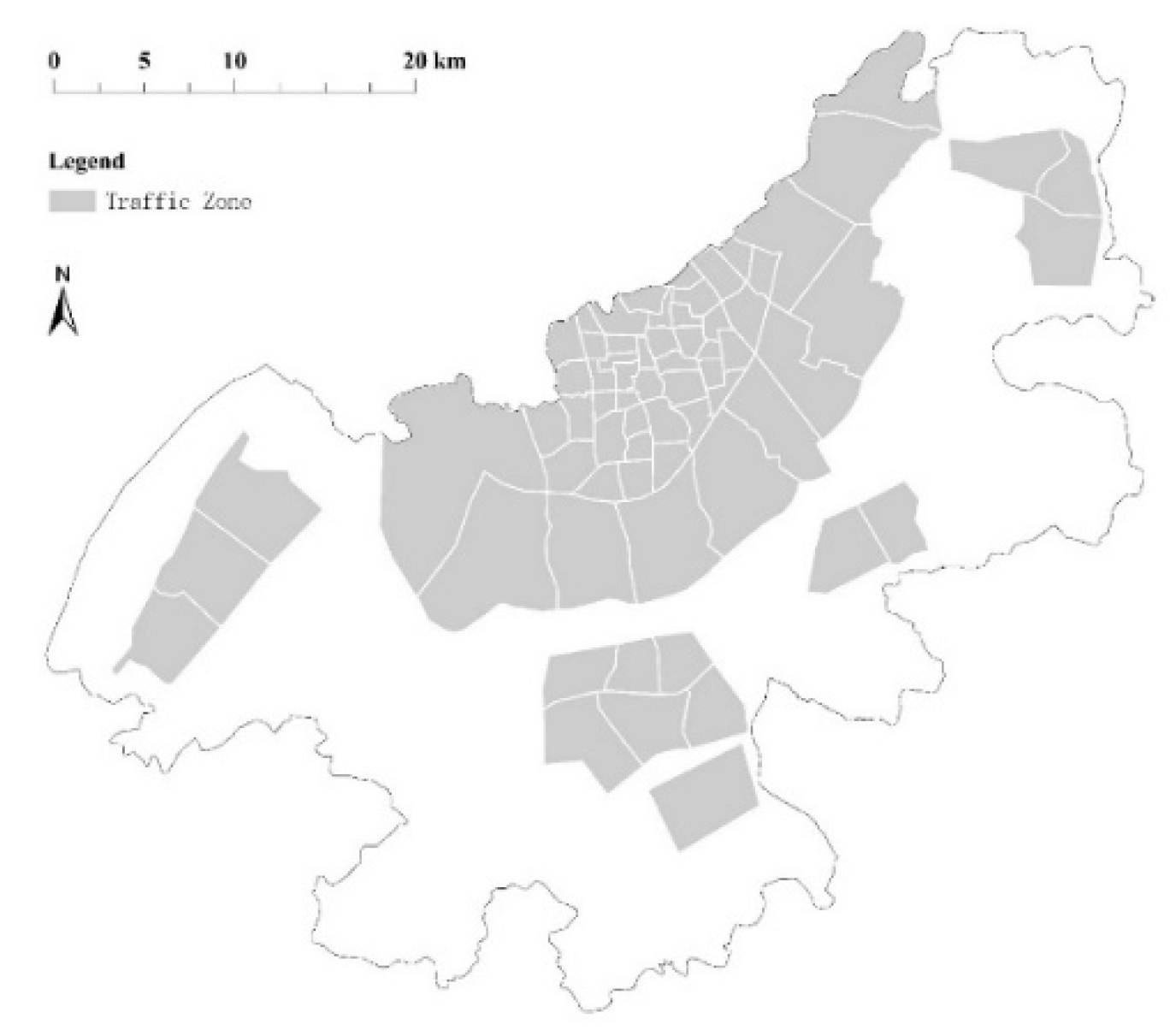
The household-related data and individual trip data used in this study were obtained from the household travel survey conducted in the Jiangning District of Nanjing, China, in 2014. Jiangning District, located in south of Nanjing, is the largest district in Nanjing with a total area of 1577.75 km² and 1,183,200 residents in 345,255 households at the end of 2014 (see Figure 1). The grey blocks in Figure 1 represent the division of Traffic Analysis Zone (TAZ) in the area of urban construction land. TAZ is the geographical division system developed specifically for transportation planning [20]. The questionnaires were developed by the research group of the urban transportation planning of Jiangning District of Nanjing City. The surveys were conducted by the research group for developing the transportation planning of Jiangning District. In the household travel survey, a total of 2802 household questionnaires were qualified for the following data analysis. The surveyed households were well distributed across the whole Jiangning District.

3. Methodologies

3.1. Emission Estimation Method

According to the Technical Guidelines for Air Pollutant Emission Inventory Compilation of Road Vehicles [21], vehicle emissions of CO, NO_x and PM_2.5 for each trip can be calculated using travel distance and emission factors. The formula for calculating the above three emissions is given as:

$$E_{j,k}{=MEF}_{j,k}\times L$$

(1)

where $E_{j,k}$ represents the vehicle emission of one trip for traffic mode j and average speed interval k; ${MEF}_{j,k}$ denotes the corresponding weighted emission factor; and L denotes the travel distance.

The travel distance L is equal to the length of the shortest path between the centroids of origin and destination TAZs, which can be calculated in ArcGIS using road net and the TAZ layer. Based on the departure and arrival time recorded in the survey, the average speed can be estimated. The value of average speed interval k can be then determined. As for travel mode, it includes walking, non-motorized vehicles like bikes or e-bikes, driving private cars, driving motorcycles, taking private cars, taking the bus and taking a taxi. For the travel modes of walking, non-motorized vehicles, and the subway, the ${MEF}_{j,k}$ is equal to zero. The weighted emission factor ${MEF}_{j,k}$ for the rest of the travel modes can be calculated by the following formula:

$${MEF}_{j,k}=\frac{{{\displaystyle \sum }}^{\text{}}E{F}_{i,k}\times c_i}{a_j{{\displaystyle \sum }}^{\text{}}{c}_i}$$

(2)

where $E{F}_{i,k}$ is the emission factor of the ith type of motor vehicle in speed interval k; $c_i$ denotes the amount of the ith type of motor vehicle in the surveyed year and place. As for motor vehicle type of different travel mode, bus includes diesel bus, pure electric bus and hybrid bus, taxi includes gasoline taxi, diesel taxi, pure electric taxi and hybrid taxi; motorcycle defaults to moped using gasoline; and private car defaults to light vehicle using gasoline. $a_j$ represents the number of passengers who share responsibility for the vehicle emission using travel mode j. If the travel mode is by bus, $a_j=80$, i.e., the personnel quota of a medium-size bus from the Standard for Classification of Urban Public Transportation [22]. If the travel mode is taking a private car, $a_j=2$ which means there are at least two persons in one car and passengers are responsible for half of the vehicle emission at most. If the travel mode is driving a private car alone, driving a motorcycle alone or taking a taxi, $a_j=1$.

The emission factors of different types of motor vehicles are calculated using the following equation:

$$E{F}_{i,k}=BE{F}_i\times \phi \times {\gamma }_k\times {\lambda }_i\times {\theta }_i$$

(3)

where $BE{F}_i$ represents baseline emission factor of the ith type of motor vehicle in speed interval k; $\phi$ is the city’s environmental correction factor; ${\gamma }_k$ denotes the speed correction factor of speed interval k; ${\lambda }_i$ denotes the deterioration correction factor of the ith type of motor vehicle; ${\theta }_i$ represents the correction factor of other use conditions of the ith type of motor vehicle. All the correction factors mentioned above refer to the National Stage IV Motor Vehicle Pollutant Emission Standard of China which can be found in the Technical Guidelines for Air Pollutant Emission Inventory Compilation of Road Vehicles [21].

3.2. Multiple Linear Regression

Multiple linear regression was used to link household daily traffic emissions with various household characteristic variables. The regression model can be expressed in matrix form as follows:

$${\mathit{Y}}_{n\times 1}={\mathit{X}}_{n\times m}{\mathit{\beta }}_{m\times 1}+{\mathit{\epsilon }}_{n\times 1}$$

(4)

$$\mathit{\epsilon }~N\left(0,{\sigma }^2\right)$$

(5)

where Y is the vector of household emissions, i.e., dependent variable; $\mathit{X}$ is an $n\times m$ matrix of household characteristic variables (see Table 4); n is the number of observation; m is the number of parameter; $\mathit{\beta }$ is the vector of m parameters for the household characteristics variables; and $\mathit{\epsilon }$ is the vector of unknown disturbance term [23].

The ordinary least squares method was used to estimate the coefficients of included household characteristic variables. Assuming that $\widehat{\mathit{\beta }}$ denote the estimates of $\mathit{\beta }$, then the equation can be written as:

$$\widehat{\mathit{\beta }}={\left({\mathit{X}}^{\mathrm{T}}\mathit{X}\right)}^{-1}{\mathit{X}}^{\mathrm{T}}\mathit{Y}$$

(6)

R-square and adjusted R-square indexes are used to measure the fitness of model in capturing the relationship between household characteristics and emissions. They are given by:

$$R^2=1-SSE/SST$$

(7)

$$R_{adjusted}^2=1-\left(\frac{n-1}{n-m}\right)\frac{\mathrm{SSE}}{\mathrm{SST}}$$

(8)

where SSE denotes the sum of square errors; SST represents the total sum of squares. F-test is used to check whether the entire regression model is significant. For testing the null hypothesis:

$$H_0:all{\beta }_j=0$$

(9)

versus

$$H_a:notall{\beta }_j=0$$

(10)

$H_0$ can be rejected if:

$$F=\frac{SSR/\left(m-1\right)}{SSE/\left(n-m\right)}>F_{\alpha }\left(\mathrm{m}-1,\mathrm{n}-\mathrm{m}\right)$$

(11)

where $\alpha$ is the level of significance and $F_{\alpha }\left(\mathrm{m}-1,\mathrm{n}-\mathrm{m}\right)$ is the 100(1 − α) % percentile of F-distribution with degrees of freedom m − 1 and n − m.

4. Data Analysis

4.1. Households’ Vehicle Exhaust Emissions

The total emissions of CO, NO_x and PM_2.5 for each household were calculated.

Table 1. Descriptive statistics of household emissions.

Descriptive Statistics	Total Emissions (g)		CO Emissions (g)		NOx Emissions (g)		PM2.5 Emissions (g)
	All	Without 0 Emission	All	Without 0 Emission	All	Without 0 Emission	All	Without 0 Emission
Sample size n	2802	1679	2802	1679	2802	1679	2802	1679
Median	3.51	11.71	2.59	11.07	0.25	0.66	0.02	0.05
Mean	9.25	15.44	8.66	14.45	0.55	0.92	0.04	0.07
Interquartile range	14.22	15.89	13.38	15.32	0.79	0.88	0.06	0.06
Minimum	0	0.15	0	0.05	0	0.02	0	0.002
Maximum	105.95	105.95	101.78	101.78	8.42	8.42	0.50	0.50
Standard deviation	13.18	13.94	12.59	13.45	0.83	0.90	0.06	0.06
Skewness	2.30	2.02	2.30	1.96	2.84	2.58	2.30	2.16
Kurtosis	7.89	6.58	7.84	6.27	12.44	10.29	8.23	7.65

gives the descriptive statistics of households’ daily vehicle emissions. The mean of daily traffic emissions of CO, NO_x and PM_2.5 per household for the whole samples are 8.66 g, 0.55 g and 0.04 g respectively. Among the total of 2802 households, 1123 households have no emissions. After excluding the samples of zero emission households, the average daily traffic emissions of CO, NO_x and PM_2.5 per household for the non-zero emission samples are 14.45 g, 0.92 g and 0.07 g respectively.

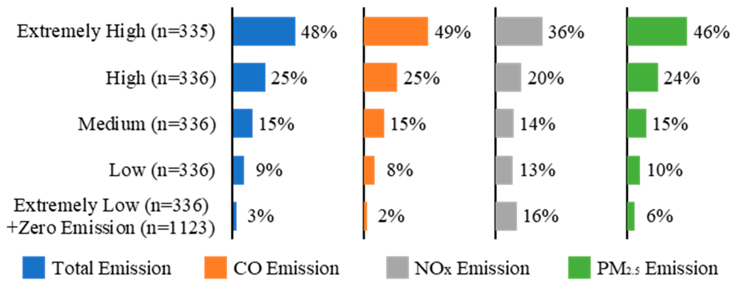
Based on the total emissions, the households were classified into six groups, including the extremely high (n = 335), high (n = 336), medium (n = 336), low (n = 336), extremely low (n = 336) and zero emission (n = 1123) group. As shown in Figure 2, the 335 households from the extremely high group contribute the 49%, 36% and 46% of the CO, NO_x and PM_2.5 emissions in the whole sample respectively. While the 1459 households from the extremely low and zero emission group only account for the 2%, 16% and 6% of the CO, NO_x and PM_2.5 emissions in the whole sample. This indicates the imbalanced distributions of emissions over households. What needs to be explained is that for the households from the low and extremely low emission group, the percentage of NO_x emissions is obviously higher than the percentages of CO, and PM_2.5. The reason is that the low-emission households are more likely to travel by bus. NO_x emissions are mainly generated by diesel vehicles like buses.

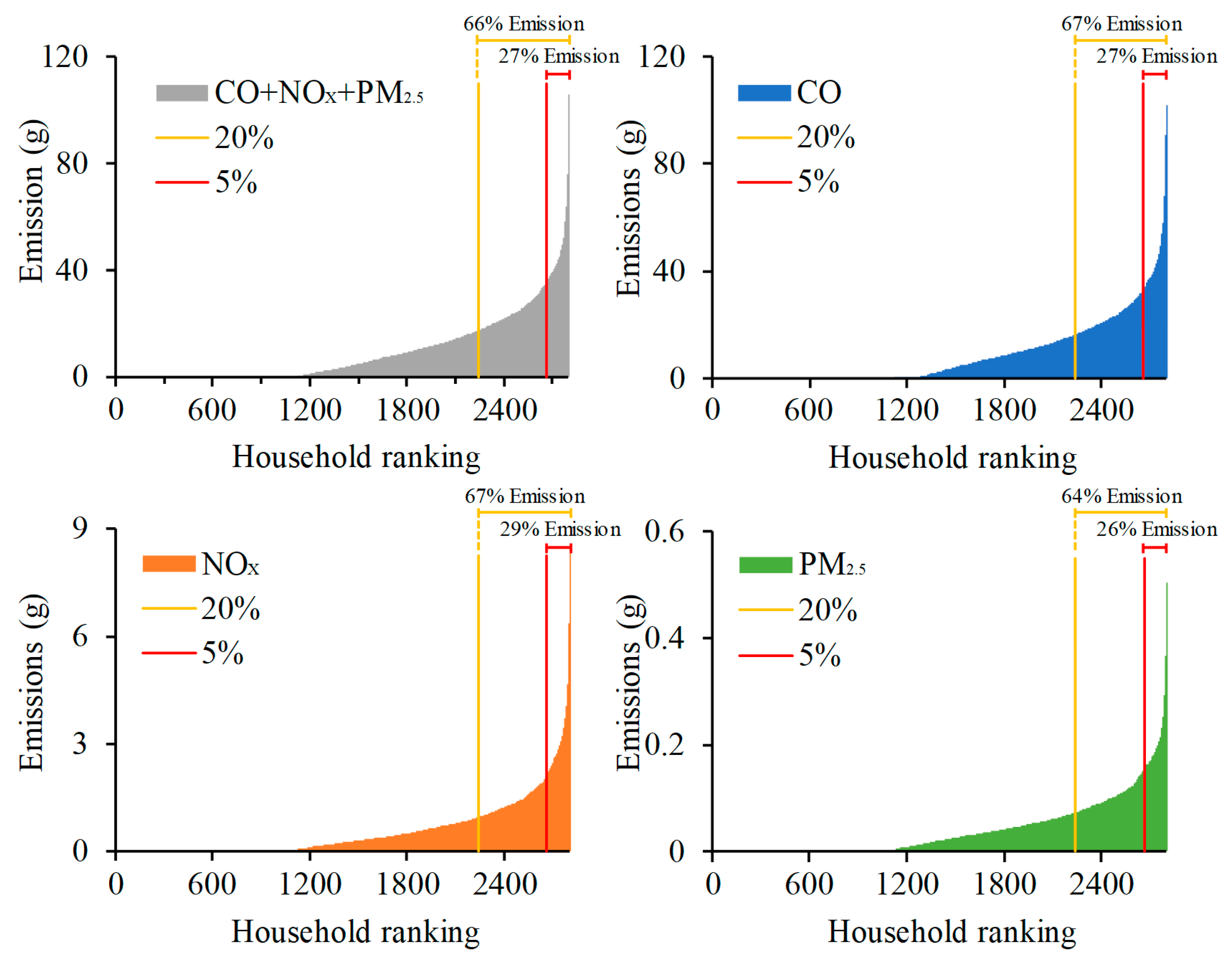
To more clearly investigate the imbalanced distributions of emissions over households, the traffic emission rankings of all households are illustrated in Figure 3. It can be found that the top 5% high-emission households were responsible for about 27% total emissions, and the top 20% were responsible for nearly two thirds of the total emissions. This suggests that policy towards households with high traffic emissions is necessary and would achieve considerable results.

4.2. Preliminary Analysis of Household Characteristics

A preliminary analysis was conducted to investigate the effects of the household characteristics on CO, NO_x and PM_2.5 emissions. One-way ANOVA tests were conducted to identify if the number of household member, household automobile number, household annual income and access to subway significantly affect the household vehicle emissions. To conduct the one-way ANOVA tests, all these four factors were classified into three groups (see

Table 2. Classification of household characteristics for one-way ANOVA tests.

Variable	Class 1	Class 2	Class 3
Household member	1~2	3~4	5~10
Automobile number	0	1	2~4
Household income	0~80,000 RMB	80,000~160,000 RMB	>160,000 RMB
Access to subway	<5 min	5~15 min	>15 min

). The cut-off selection for each class was based mainly on social status in China to make each class representative. More specifically, the number of household member was classified into three groups, including households with one or two members which usually do not have children, three or four members which may consist of parents and one or two children, and more than four members which may be a large family with grandparents together. The cut-off values for the other three factors are given Table 2.

Table 3. One-way ANOVA tests of household characteristics.

Test Factor	CO		NOx		PM2.5
	F	Sig.	F	Sig.	F	Sig.
Household member	84.28	<0.001	46.37	<0.001	91.78	<0.001
Automobile numbers	501.48	<0.001	99.67	<0.001	480.28	<0.001
Household income	160.98	<0.001	41.09	<0.001	149.49	<0.001
Access to subway	5.38	0.004	2.38	0.092	5.54	0.004

gives the results of the one-way ANOVA tests for CO, NO_x and PM_2.5 emissions for each of the four factors. All the test results are of the significant level of 0.05 or 0.1, indicating that the means of CO, NO_x and PM_2.5 emissions are significantly different over the groups defined by each of the four factors.

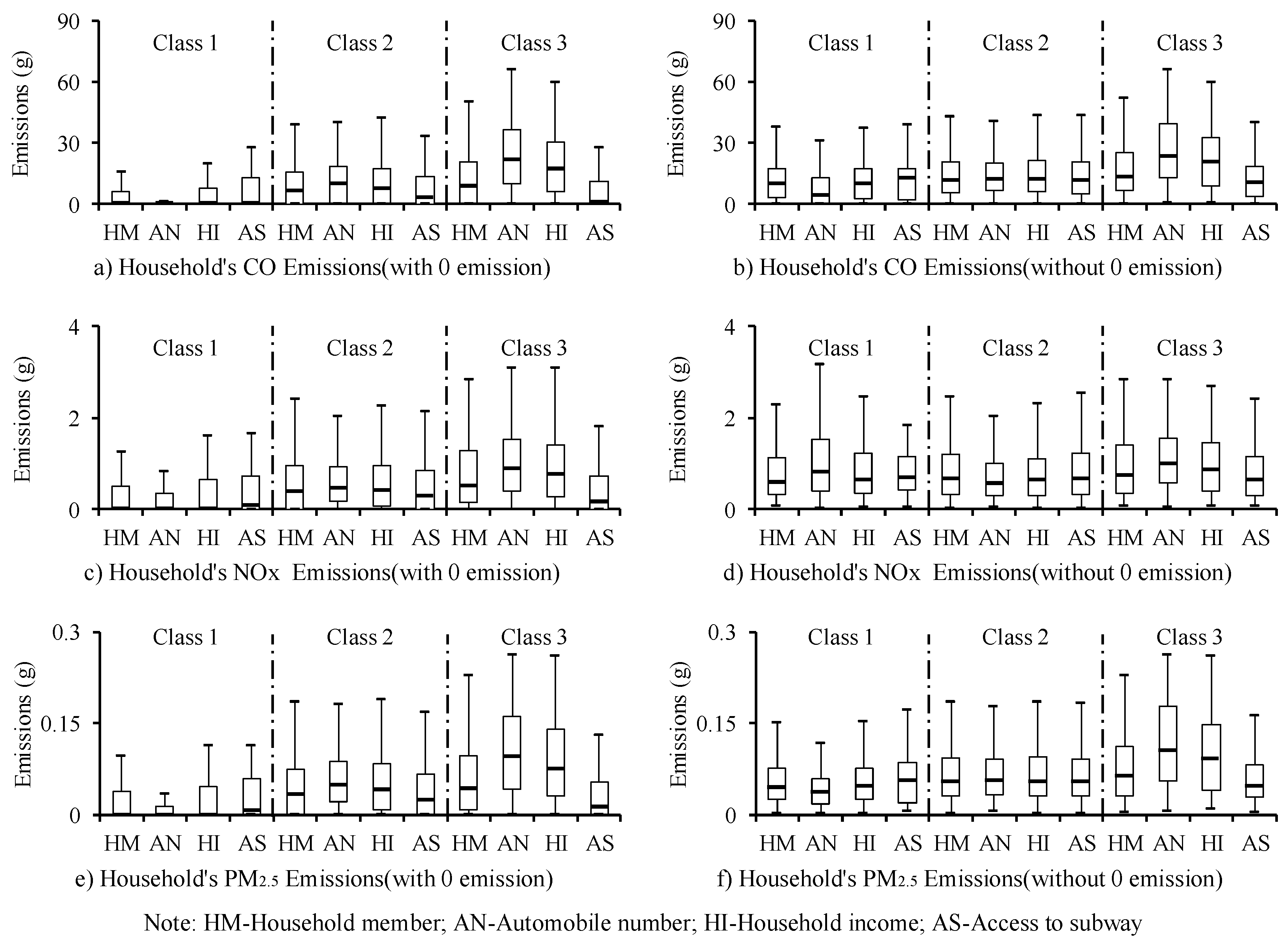
To more clearly illustrate the relationship between vehicle emissions and household characteristics, the box plots were developed for CO, NO_x and PM_2.5 emissions for each of the four factors (see Figure 4). As expected, the means of all the three emissions increase with an increase in the number of household members. With regard to household automobile numbers and annual income, the means of CO, NO_x and PM_2.5 emissions are positively related with household automobile numbers and annual income.

As shown in Figure 4, one interesting finding is that better access to the subway does not lead to obvious reductions in all of the three emissions. In fact, the mean emissions of the households with shorter times to subway stations are slightly higher than those of the households with longer times to subway stations. This result indicates that people living near to subway stations are still likely to use private automobiles. The house properties near to the subway stations generally have higher prices. People living near subway stations tend to have higher income. Accordingly, they are more likely to travel by private automobile.

4.3. Regression Analysis of Household Characteristics

Multiple linear regression models were developed to link the vehicle emissions with household characteristics.

Table 4. Description of independent variables.

Variable	Description
HM (Household members)	Number of household members:
	1—if it is 1 or 2;
	2—if it is 3 or 4;
	3—others
RsdPop (Resident population)	Number of resident population
Worker	Number of people with jobs
TmpPop (Temporary population)	Temporary population in a household
SqrTmpPop (Square of temporary population)	Square of temporary population in a household
Child	Number of children in a household
Bike	Number of bicycles in a household
eBike	Number of electric bicycles in a household
NonMotor	Sum of bicycles and electric bicycles in a household
Motor	Number of motorcycles in a household
AN (Automobile vehicle number)	Number of private cars in a household
PSpc (Parking space)	Number of parking spaces in a household
Auto-PSpc (Automobile vehicle number×Parking space)	Number of private cars times number of parking spaces
HI (Household Income)	Household Income:
	1—if it is less than 40,000 RMB;
	2—if it is between 40,000 and 80,000 RMB;
	3—if it is between 80,000 and 120,000 RMB;
	4—if it is between 120,000 and 160,000 RMB;
	5—if it is between 160,000 and 200,000 RMB;
	6—if it is more than 200,000 RMB
CRBld (Residential building)	Housing type:
	1—if it is commercial residential building;
	0—others
ResettleHse (Commercial resettlement housing)	Housing type:
	1—if it is commercial resettlement housing;
	0—others
AffHse (Affordable housing)	Housing type:
	1—if it is affordable housing;
	0—others
Villa	Housing type: 1—if it is Villa; 0—others
Tenement	Housing type: 1—if it is Tenement; 0—others
BusAccs (Bus access)	Walking time to the nearest bus stop: 1—if it is less than 5 min; 2—if it is between 5 and 10 min; 3—if it is between 10 and 15 min; 4—if it is more than 15 min
AS (Access to subway)	Walking time to the nearest subway station: 1—if it is less than 5 min; 2—if it is between 5 and 10 min; 3—if it is between 10 and 15 min; 4—if it is more than 15 min

gives the candidate variables for model development. Multicollinearity might bias the results of multiple linear regressions. To avoid the biased results caused by multicollinearity, the research team calculated the Pearson correlation parameters between different candidate variables and generated several combinations which included the maximum number of uncorrelated variables. The combination of maximum uncorrelated variables with the best R² was used to develop the final multiple linear regression models. The Pearson correlation coefficients between final significant variables are listed in

Table 5. Pearson correlation coefficients between selected variables.

	HM	Worker	TmpPop	SqrTmpPop	Child	eBike	NonMotor
HM	1.000
Worker	0.398	1.000
TmpPop	0.108	−0.043	1.000
SqrTmpPop	0.177	−0.002	0.6948	1.000
Child	0.374	0.010	0.042	0.073	1.000
eBike	0.260	0.284	−0.012	0.017	0.008	1.000
NonMotor	0.315	0.326	−0.059	−0.026	0.020	0.794	1.000
Motor	0.015	0.106	<0.001	0.015	−0.074	0.025	0.077
AN	0.216	0.166	−0.118	−0.078	0.1177	−0.040	0.002
HI	0.129	0.132	−0.055	−0.031	0.112	−0.095	−0.082
CRBld	0.006	0.007	−0.291	−0.245	0.086	−0.037	0.018
Villa	0.015	0.012	−0.047	−0.039	−0.029	−0.040	−0.041
Tenement	−0.163	−0.100	0.596	0.506	−0.066	−0.073	−0.139
BusAccs	0.011	0.003	0.012	0.008	0.013	0.028	−0.013
	Motor	AN	HI	CRBld	Villa	Tenement	BusAccs
HM
Worker
TmpPop
SqrTmpPop
Child
eBike
NonMotor
Motor	1.000
AN	−0.203	1.000
HI	−0.118	0.375	1.000
CRBld	−0.128	0.186	0.255	1.000
Villa	−0.026	0.131	0.146	−0.110	1.000
Tenement	0.031	−0.236	−0.159	−0.478	−0.050	1.000
BusAccs	0.095	−0.082	0.019	−0.143	0.040	−0.001	1.000

. And

Table 6. Multiple Linear Regression Models of Household Emissions.

Variables	CO Emissions a		NOx Emissions a		PM2.5 Emissions a
	Coef.	Std. Err.	Coef.	Std. Err.	Coef.	Std. Err.
Constant	0.536	0.115	−0.921	0.105	−3.886	0.085
HM	-	-	0.079	0.027	-	-
Worker	-	-	0.087	0.035	0.095	0.030
TmpPop	−0.199	0.094	-	-	-	-
SqrTmpPop	0.068	0.028	-	-	-	-
Child	-	-	−0.099	0.051	-	-
eBike	-	-	−0.141	0.034	−0.101	0.029
NonMotor	−0.066	0.031
Motor	0.738	0.079	0.173	0.061	0.158	0.054
AN	1.085	0.057	−0.117	0.045	0.441	0.039
HI	0.099	0.028	0.046	0.021	0.050	0.019
CRBld	0.176	0.063	-	-	0.112	0.042
Villa	-	-	-	-	0.384	0.191
Tenement	-	-	0.131	0.060	-	-
BusAccs	0.148	0.037	0.065	0.028	0.099	0.026

Note: ^a Natural logarithmic transformation.

gives the estimation results of the final models for CO, NO_x and PM_2.5 emissions.

4.3.1. Impacts of Household Characteristics on CO Emissions

There are eight variables in the final model for CO emissions. The variables SqrTmpPop, Motor, AN, HI, CRBld and BusAccs all have positive impacts on CO emissions, while the variables TmpPop and NonMotor are negatively correlated with CO emissions.

The coefficients of temporary population in a household (represented by TmpPop) and its quadratic terms (represented by SqrTmpPop) indicate a nonlinear relationship between CO emissions and temporary population in a household. The CO emissions first decrease with an increase in temporary population in a household, and then increase as the temporary population increase. Regarding the vehicle ownership, the number of bicycles and electric bicycles in a household leads to reduced CO emissions. As indicated by the coefficients of Motor and AN, the CO emissions increase with an increase in the number of motorcycle and private cars in a household.

With regard to the housing type, it can be found that commercial residential building housing leads to higher CO emissions. The coefficient of HI is positive, indicating that households with higher annual incomes generate relatively larger CO emissions. The coefficient of BusAccs is positive, indicating that the CO emissions increase with an increase in the walking time to the nearest bus stop. This result is intuitive that people live far away from bus stops are more likely to take motorized vehicles, such as primary cars.

4.3.2. Impacts of Household Characteristics on NO_x Emissions

In the model of NO_x emissions, nine variables significantly affect the amount of household NO_x emissions. The variables HM, Worker, Motor, HI, Tenement and BusAccs all have positive impacts on NO_x emissions, while the variables Child, eBike and AN are all negatively correlated with NO_x emissions.

The coefficients of variables HM and Worker indicate that the amount of NO_x emissions increases as the numbers of household members and workers increase. With regard to the vehicle ownership, large number of electric bicycles was found to be associated with the decrease in NO_x emissions. The coefficient of AN is negative, indicating that the NO_x emission decreases with an increase in the number of private cars. One possible reason for this result is that, in the household without private cars, people are likely to travel by public buses. As mentioned above, diesel vehicles such as buses have much higher emission factor of NO_x emissions than private cars. The coefficient of HI indicates that the household income is positively correlated with the amount of NO_x emissions.

With regard to the housing type, the coefficient of Tenement is positive, implying that the households with rented apartment have higher NO_x emissions. This result is intuitive that the household members are likely to travel by public buses. The positive coefficient of BusAccs indicates that the amount of NO_x emissions increase with an increase in the walking time to the nearest bus stop. People live far away from bus stop might use motorcycles, resulting in higher NO_x emissions.

4.3.3. Impacts of Household Characteristics on PM_2.5 Emissions

In the model of PM_2.5 emissions, eight variables significantly affect the amount of household PM_2.5 emissions. The variables Worker, Motor, AN, HI, CRBld, Villa and BusAccs all have positive impacts on PM_2.5 emissions. Only the variable eBike has a negative effect on PM_2.5 emissions.

The coefficient of Worker indicates that the number of workers in a household is positively correlated with PM_2.5 emissions. As expected, the amount of PM_2.5 emissions increases with an increase in the motorcycle and private cars in a household. The number of electric bicycles was found to be negatively correlated with PM_2.5 emissions. The household annual income is positively associated with PM_2.5 emissions. With regard to the housing type, both commercial residential buildings and villas have positive correlations with PM_2.5 emissions. The coefficient of BusAccs is also positive in the model of PM_2.5 emissions, indicating that the amount of household PM_2.5 emissions increases with an increase in the distance between the dwelling place and the nearest bus stop.

Comparing the results of the three regressions, the contributing factors are slightly different among the three different emissions. The number of motorcycles, number of private cars, and household income significantly affect all three emissions. The number of motorcycles in a household has positive effect on all three emissions. The number of private cars in a household has a positive effect on the CO and PM_2.5 emissions, but a negative effect on the NOx emissions. The household income is positively correlated with the amount of all three emissions.

5. Conclusions

This study aimed to investigate the effects of household characteristics on household vehicle emissions. Based on the household travel survey data, the vehicle emissions of household members’ trips were calculated by the average speed emission factors. Statistics tests and multiple linear regression were then conducted to evaluate the effects of household characteristics on household daily traffic emissions. The following conclusions are made on the basis of the data analysis results:

(1) The average daily emissions of CO, NO_x and PM_2.5 per household for all samples are 8.66 g, 0.55 g and 0.04 g respectively. The average daily traffic emissions of CO, NO_x and PM_2.5 per household for the non-zero emission samples are 14.45 g, 0.92 g and 0.07 g, respectively. The household emissions were found to have imbalanced distributions over households. The top 5% high-emission households were responsible for about 27% total emissions, and the top 20% high-emission households were responsible for nearly two thirds of the total emissions.

(2) The one-way ANOVA tests indicated that the means of CO, NOx and PM_2.5 emissions are significantly different over households with different member number, automobile number, annual income and access to the subway. The number of household members was found to be positively correlated with all three emissions. The household automobile number and annual income were found to have positive effects on all three emissions. The households with better access to the subway do not have obvious lower daily traffic emissions.

(3) To further investigate the effects of household characteristics on the three emissions, the multiple linear regression model was developed for each pollutant. The results suggested that the contributing factors are slightly different across the three different emissions. More specifically, the number of bicycles has negative effects on CO emissions. The household income, motorcycle number, private car number and access to public transport were found to have positive effect on CO emissions. In the regression model for the NOx Emissions, the household members, worker number, motorcycle number, household income, and bus stop access have positive effects. The numbers of e-bikes and private cars were found to be negatively correlated with NOx Emissions. The regression analyses of PM_2.5 emissions indicated that the number of e-bikes has a negative effect on PM_2.5 emissions. The number of workers, number of motorcycles and private cars, household annual income, commercial residential buildings and villas, and access to public transport were found to have positive effects on PM_2.5 emissions.

The results of this study were obtained based on the data from the Nanjing City, which is a typical second-tier city in China. Although these results might not be directly applicable to other type cities, the modeling framework of this study can be directly transferred to other type cities. When the data from other cities are available, the used framework in this study can be easily used to reveal the new results. A future study might focus on comparing the results of different types of cities.

References

- National Bureau of Statistics of China. China Statistical Yearbook; Chinese Statistics Press: Beijing, China, 2008–2017.
- Health Effects Institute. Panel on the Health Effects of Traffic-Related Air Pollution. In Traffic-Related Air Pollution: A Critical Review of the Literature on Emissions, Exposure, and Health Effects; Health Effects Institute: Boston, MA, USA, 2010. [Google Scholar]
- Ministry of Ecology and Environment of the People’s Republic of China. China Vehicle Environmental Management Annual Report; Ministry of Ecology and Environment of the People’s Republic of China: Beijing, China, 2018.
- Bachman, W.H. A GIS-Based Modal Model of Automobile Exhaust Emissions; United States Environmental Protection Agency, Research and Development, National Risk Management Research Laboratory: Washington, DC, USA, 1998.
- Huang, Q.; Yu, L.; Yang, F.; Song, G. A Synthesis of Mobile Emission Evaluation Models. Environ. Prot. Transp. 2003, 6, 14. [Google Scholar]
- Franco, V.; Kousoulidou, M.; Muntean, M.; Ntziachristos, L.; Hausberger, S.; Dilara, P. Road vehicle emission factors development: A review. Atmos. Environ. 2013, 70, 84–97. [Google Scholar] [CrossRef]
- Hao, L.; Chen, W.; Li, L.; Tan, J.; Wang, X.; Yin, H.; Ding, Y.; Ge, Y. Modeling and predicting low-speed vehicle emissions as a function of driving kinematics. J. Environ. Sci. 2017, 55, 109–117. [Google Scholar] [CrossRef] [PubMed]
- Pouresmaeili, M.A.; Aghayan, I.; Taghizadeh, S.A. Development of Mashhad driving cycle for passenger car to model vehicle exhaust emissions calibrated using on-board measurements. Sustain. Cities Soc. 2018, 36, 12–20. [Google Scholar] [CrossRef]
- D’Angelo, M.; González, A.E.; Tizze, N.R. First approach to exhaust emissions characterization of light vehicles in Montevideo, Uruguay. Sci. Total Environ. 2018, 618, 1071–1078. [Google Scholar] [CrossRef] [PubMed]
- Huang, Y.; Organ, B.; Zhou, J.; Surawski, N.C.; Hong, G.; Chan, E.F.C.; Yan, Y.S. Emission measurement of diesel vehicles in Hong Kong through on-road remote sensing: Performance review and identification of high-emitters. Environ. Pollut. 2018, 237, 133–142. [Google Scholar] [CrossRef]
- Yusoff, M.; Zulkifli, N.W.M.; Masjuki, H.H.; Harith, M.H.; Syahir, A.Z.; Khuong, L.S.; Zaharin, M.S.M.; Alabdulkarem, A. Comparative assessment of ethanol and isobutanol addition in gasoline on engine performance and exhaust emissions. J. Clean. Prod. 2018, 190, 483–495. [Google Scholar] [CrossRef]
- Boriboonsomsin, K.; Durbin, T.; Scora, G.; Johnson, K.; Sandez, D.; Vu, A.; Jiang, Y.; Burnette, A.; Yoon, S.; Collins, J.; et al. Real-world exhaust temperature profiles of on-road heavy-duty diesel vehicles equipped with selective catalytic reduction. Sci. Total Environ. 2018, 634, 909–921. [Google Scholar] [CrossRef] [PubMed]
- Durand, T.; Eggenschwiler, P.D.; Tang, Y.; Liao, Y.; Landmann, D. Potential of energy recuperation in the exhaust gas of state of the art light duty vehicles with thermoelectric elements. Fuel 2018, 224, 271–279. [Google Scholar] [CrossRef]
- Mendoza-Villafuerte, P.; Suarez-Bertoa, R.; Giechaskiel, B.; Riccobono, F.; Bulgheroni, C.; Astorga, C.; Perujo, A. NOx, NH3, N2O and PN real driving emissions from a Euro VI heavy-duty vehicle. Impact of regulatory on-road test conditions on emissions. Sci. Total Environ. 2017, 609, 546–555. [Google Scholar] [CrossRef] [PubMed]
- Huang, Y.; Ng, E.C.Y.; Zhou, J.; Surawski, N.C.; Chan, E.F.C.; Hong, G. Eco-driving technology for sustainable road transport: A review. Renew. Sustain. Energy Rev. 2018, 93, 596–609. [Google Scholar] [CrossRef]
- Kim, W.G.; Kim, C.K.; Lee, J.T.; Kim, J.; Yun, C.; Yook, S. Fine particle emission characteristics of a light-duty diesel vehicle according to vehicle acceleration and road grade. Transp. Res. Part D Transp. Environ. 2017, 53, 428–439. [Google Scholar] [CrossRef]
- Liu, Z. Road Alignment Index Evaluation with Vehicle Pollution and Fuel Consumption; Southeast University: Nanjing, China, 2017. [Google Scholar]
- Zhou, H. Study on Traffic emission (CO) Pollution at Intersections. J. Tongji Univ. 1996, 24, 642–646. [Google Scholar]
- Sobrino, N.; Monzon, A. Management of Urban Mobility to Control Climate Change in Cities in Spain. Transp. Res. Rec. J. Transp. Res. Board 2013, 2735, 55–61. [Google Scholar] [CrossRef]
- Bao, J.; Xu, C.; Liu, P.; Wang, W. Exploring Bikesharing Travel Patterns and Trip Purposes Using Smart Card Data and Online Point of Interests. Netw. Spat. Econ. 2017, 17, 1231–1253. [Google Scholar] [CrossRef]
- Ministry of Ecology and Environment of the People’s Republic of China. Technical Guidelines for Air Pollutant Emission Inventory Compilation of Road Vehicles (Trial). Available online: http://www.zhb.gov.cn/gkml/hbb/bgg/201501/W020150107594587831090.pdf (accessed on 31 December 2014).
- Ministry of Construction of China. Standard for Classification of Urban Public Transportation (CJJ/T 114-2007); China Architecture & Building Press: Beijing, China, 2007.
- Xu, C.; Wang, Y.; Liu, P.; Wang, W.; Bao, J. Quantitative risk assessment of freeway crash casualty using high-resolution traffic data. Reliab. Eng. Syst. Saf. 2018, 169, 299–311. [Google Scholar] [CrossRef]
Figure 1.
Traffic zone and sample household distribution.
Figure 2.
Household emissions by low, medium and high groups.
Figure 3.
Vehicle emissions rankings of all households.
Figure 4.
Box plots of household’s emissions.