On the Relationship between Economic Policy Uncertainty and the Implied Volatility Index


Department of Accounting and Finance, Management Development Institute Gurgaon, Gurugram 122001, Haryana, India
Sustainability 2019, 11(6), 1628; https://doi.org/10.3390/su11061628
Submission received: 28 January 2019
/
Revised: 14 February 2019
/
Accepted: 6 March 2019
/
Published: 18 March 2019
(This article belongs to the Special Issue Application of Time Series Analyses in Business)
Abstract
:This article examines the effects of economic policy uncertainty (EPU) on the implied volatility index. The implied volatility index of various markets has been analyzed in relation to scheduled macroeconomic announcements, such as EPU and equity market policy uncertainty (EMPU) indices. The study highlights that EPU contains important information to explain the diverse market effects of the U.S., which is gauged into the volatility index. Estimates obtained in an autoregressive conditional heteroscedasticity framework indicate the persistence of volatility during spikes in the EPU. More importantly, the lagged values of the policy uncertainty index also contains market-related information to explain the markets’ future volatility. Major political and economic events have also contributed positively in that a presidential election contains information to explain various asset classes. Commodities, such as crude oil, gold, corn, and soybean, have been impacted significantly followed by EPU. Moreover, interest rate market volatility has also been moved adversely due to tight monetary policy. The Markov regime switching regression manifests that the implied volatility index (VIX) behaves abruptly in two different regimes followed by EPU.
1. Introduction
Baker et al. [1] have built an index of policy uncertainty for the U.S. economy. Economic policy uncertainty (EPU) is an outlook of the U.S. economy that expresses about changes in the prevailing economic policies that govern the directions of the economic game in terms of non-zero probability for the market participant. Policy uncertainty tends to change in light of the ‘delay’ in the economic and political decisions. It should be noted that policy uncertainty not only affects future investment, consumption, and employment, but also the cost of production and financing, and supply chain networks. The asset price is affected by policy uncertainty, which is the reason it commands both interest rate and risk-premium (e.g., Pastor and Veronesi, [2,3]; Amidu and Adjasi, [4]; Liao et al., [5]).
Christou et al. [6] examined the effects of policy uncertainty on stock returns in a panel vector auto regression (VAR) setting for Pacific Rim countries. Empirical results indicated that stock market returns have significant negative effects with regard to the increased levels of policy uncertainty. The U.S.-specific policy uncertainty negatively affected countries under their study, excluding Australia. Raza et al. [7] examined the equity premium for the G7 countries based on monthly data under economic policy uncertainty using quantile-on-quantile regression. They reported a negative association between the quantile of EPU and quantile of equity premium and the estimates also signaled a negative association for extremely low and high tails. Gábor and Georgarakos [8] conducted a survey of household stockholding and stock market participation based on policy uncertainty. After monitoring several indicators for the household stockholding, they found that households with a higher exposure level to policy-related news may less likely to invest in stocks. Indeed, such involvement is independent of the level of VIX and household expectations. Duan et al. [9] investigated the leverage effects and EPU on future stock market volatility using the regime-switching framework. On the information content of heterogenous autoregressive model of realized volatility (HAR-RV) and GARCH-class models, HAR-RV including leverage effects and EPU outperformed the traditional GARCH-class models. Hu et al. [10] put in effort to replicate the study of Bali et al. [11] in the Chinese equity market with regard to the EPU index and find China’s A-shares were significantly affected based on the U.S. EPU shocks. Furthermore, the U.S.-based EPU shocks on the Chinese market across diverse industries found to be asymmetric, and investors have to recompense a premium in order to purchase Chinese A-shares related to policy uncertainty.
Previous studies (e.g., Graham et al., [12]; Nikkinen and Sahlström, [13,14]; Nikkinen et al., [15]; Chen and Clement, [16]; Onan et al., [17]) evidently reported the information contained in the FOMC and macroeconomic news to explain the equity market volatility. These studies show the effects of the uncertainty of monetary policy and other macro data in terms of the implied volatility index (VIX). Estimates suggest that for policy uncertainty, VIX tends to rise before the information announcements and goes normal on the day of the news release. Yet, there is no empirical work in the literature that takes into consideration policy uncertainty to analyze its effects on the VIX across various specific markets.
Furthermore, studies (e.g., Reinhart and Simin, [18]; Rigobon and Sack, [19]; Farka and Fleissig, [20]; Wang and Mayes, [21]; Amidu and Adjasi, [4]) evaluate monetary policy uncertainty in the case of scheduled FOMC statements and find that changes in the Feds’ policy rates related to uncertainty effect significantly to the financial assets, including the bank’s diversification strategy and resource allocation.
Few studies (e.g., Antonakakis et al., [22]; Arouri et al., [23]; Demir et al., [24] and Gabauer and Gupta, [25]) examined co-movement between equity markets, bitcoin markets, and policy uncertainty. Theoretically, uncertainty effects of categorical EPU spillover between two countries and, hence, there is a dearth of studies on the relationship between EPU and markets’ ex ante volatility. This paper, therefore, aims to fill this research gap and add to the literature on policy uncertainty and asset pricing. A novelty of this empirical work is longer time duration, 14 volatility indices, scheduled macroeconomic announcements, major economic and political events, and presidential election uncertainty.
2. Data Description and Summary Statistics
Does policy uncertainty affect investors’ sentiment, measured by VIX? To answer this question, this study explores different VIX allied volatility measures in relation to EPU of the U.S. economy. The timeline of the empirical work covers from 2001/01 to 2018/03, and the sample varies according to the VIX of various specific markets. A total of 14 VIX-based volatility measures have been analyzed to uncover the effects of the policy uncertainty. The equity market-related volatility indices are VIX-SPX500, VXN-NASDAQ, VXO-OEX, VXD-DJIA, and VVIX-VIX. The commodity associated volatility indices are OIV-WTI, OVX-USO, GVZ-SPDR, and SIV-Soybean futures and CIV-Corn futures. The foreign exchange market encompasses EUVIX-FXE, JYVIX-FXY, and BPVIX-FXB. The interest rate volatility index reflects TYVIX-T-Note futures. The above-mentioned indices are the measures of investors’ sentiment across various assets class including volatility as one of the assets. The study employs the economic policy uncertainty (EPU) index and equity market policy uncertainty (EMPU) index of the U.S. economy available on a daily scale. Moreover, scheduled macroeconomic indicators, such as the FOMC, GDP, and other macro reports, have also been considered for the analysis (e.g., Saikia and Borbora [26] considered GDP, money supply and inflation to examine the outward foreign direct investment flows). In this paper, there are 147 FOMC meeting days, 256 GDP reports, and 2444 other macroeconomic indicators.
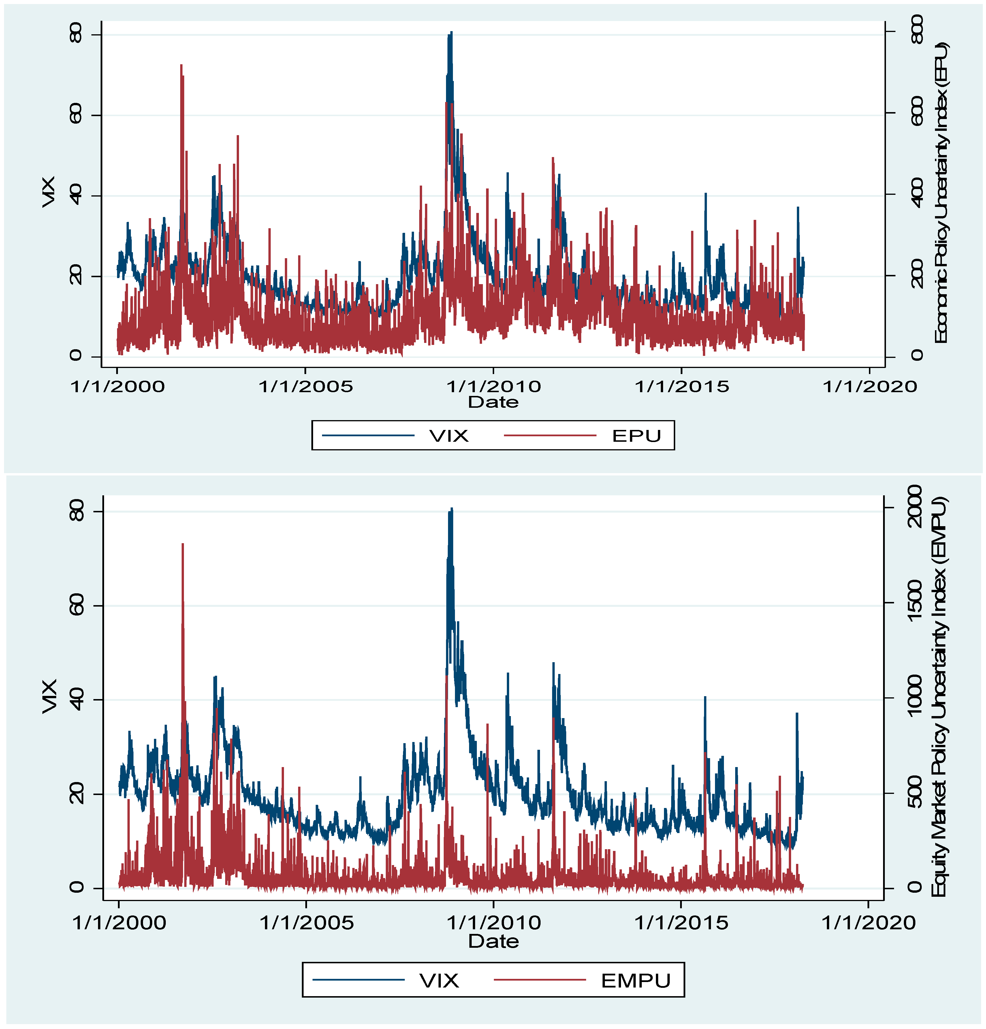
Table 1 summarizes the correlation between the policy uncertainty and implied volatility. The matrix shows the correlation for select VIX measures. The degree of association between the VIX-SPX500 and EPU appears to be highest and statistically significant on the counterpart of other markets. The association is more pronounced during the calendar years followed by a high level of uncertainty. Figure 1 exhibits a temporal relation between the VIX and EPU-EMPU. The VIX is more volatile subject to major economic and political events such as the 2000’s boom, credit crunch, global financial crises and fiscal cliff. Table 2 shows the tests of stationarity of the VIX and EPU index based on the PP-test and reject the null hypothesis ‘time series variable has unit root’ in level.
This section provides a concise and precise description of the experimental results, their interpretation, and the experimental conclusions that can be drawn.
3. Empirical Model
To examine the effects of the policy uncertainty on markets’ future volatility, a contemporaneous change in the volatility index has been calculated (e.g., Fleming et al., [27]; Shaikh and Padhi, [28]; Shaikh, [29]). A nested regression model with dependent variable is regressed over intercept terms, lagged , and a vector of scheduled macroeconomic announcements:
where:
- = intercept, measures change in the volatility during a non-announcements days, it should be “positive”
- = slope coefficient of FOMC, through −5 day “positive”, on report day “negative”, and through +5 day “negative”
- = slope coefficient of GDP, through −5 day “positive”, on report day “negative”, and through +5 day “negative”
- = slope of other macro indicators through −2 day “positive”, on report day “negative”, and through +2 day “negative”
- = dummy variable, assumes 1 on the day of report release, otherwise zero
- = represent the returns on respective underlying assets/index
- = classical error term
Engel [30] proposes the ARCH/GARCHX model under a condition that predetermined or exogenous variables exist. The ultimate aim of volatility measurement is to explain the causes of volatility. Further, Bollerslev and Melvin [31] model the uncertainty of foreign exchange market through GARCHX-type specifications. They introduce the conditional variance with {} as the ask prices and provide some new insights on the relationship between volatility and spreads. Nana et al. [32] argue that the volatility estimation with exogenous factor allows additional sources of information, showing more established markets’ behavior and reports a greater accuracy in forecasting the markets’ reactions. The volatility estimation has been performed in an autoregressive conditional heteroskedasticity by using ARCH/GARCH model. Both EPU and EMPU are stationary (see Table 2) in level and outside the system, and have been included as an exogenous regressor in variance equation (e.g., Engel, [30] and Nana et al. [32]). Moreover, dummies of the major economic and political events have also been plugged into the variance equation. Based on the framework of Nana et al. [32] GARCHX (1,1), the estimation process is defined as:
where, {} is the vector of exogenous variables EPU, EMPU, and other major economic and political events, and presidential election year. present the non-negative continuous functions. signifies a non-negative real number.
The regression model specified through Equations (1)–(3) do not regard the effects of the structural break and time-variant nature of the parameter estimated. In order to derive robust results on the relationship between policy uncertainty and implied volatility a Markov regime switching regression model expressed as:
Here, represents the change in the uncertainty variable. Moreover, lagged values of the uncertainty variable have also been included in Equation (4). is the discrete regime variable in the Markov process and assumes {1,2} in two states and (0, ).
4. Results and Discussion
Table 3 summarizes the estimates of the mean equation with regard to the scheduled macroeconomic announcement of the U.S. economy. The market participants closely follow the minutes of the FOMC committee in order to design their future investment strategy. The monetary policy uncertainty creates an ambiguity among investors and due to the lack of information on the Fed’s policy VIX tends to rise until the information is released publicly (e.g., Nikkinen and Sahlström, [13] and Nikkinen et al., [15]). Similarly, uncertainty about GDP data and other macroeconomic fundamentals affect investors’ sentiment and, consequently, VIX keeps on increasing prior to the release of information. Among the reports that are publicly available, VIX tends to adjust to its normal range.
Column (1) of Table 3 presents the behavior of 14 important markets around FOMC meeting days. It is seen that all 14 volatility indices tend to rise prior to FOMC statement releases and then goes normal on the day of the minutes releases. It is also apparent that VIX keeps on decreasing up to certain days after the monetary policy is announced. Column (2) shows the effects of GDP report on various markets of the U.S economy. Prior to the GDP declaration, it is seen that most of the markets’ expected volatility was rising marginally and it then reverted back to a normal level once the report as released. Column (3) also represents the similar outcome reported earlier. One of the key observation is that commodity and foreign exchange markets remain unaffected before the announcement of CPI, PPI, real earnings, employment situations, job openings and labor turnover, U.S. export/imports, state employment, unemployment, and so on.
Table 4 shows the estimates for variance equation with exogenous variables, such as EPU, major economic and political events, and presidential election year. The intercept, ARCH, and GARCH parameters appear to be positive and statistically significant. This implies that volatility persists in relation to policy uncertainty. The estimates on EPU and EMPU found to be statistically significant. The equity markets’ volatility tends to remain positive in relation to policy uncertainty, while the effects of policy uncertainty on commodity, foreign exchange, and interest rate volatility is found to be adverse. But equity market specific uncertainty has increased the volatility of the equity market and other markets as well. The major political and economic events have also contributed positively; presidential elections also contain information to explain various assets classes.
Based on the sample first major economic event the 2000’s commodity boom ranges from 2003/01 to 2007/06 and its impact on the equity market found to be negative and significant. The negative slope of implied volatility during this period implies that the commodity-related boom caused equity market volatility to fall until 2007/06. Moreover, other markets, such as crude oil and government securities markets, also exhibited the similar effects. The second major economic event is the ‘credit crunch’ experienced during 2007/07 to 2008/08: this is the period of the turmoil of credit market and significantly hampered the banking system through an increase in the interest rates. The equity market has remained unaffected by this early credit crunch but the crude oil market was adversely affected. Further, Table 4 clearly shows that the credit crunch significantly raised the oil price market volatility. On the other hand, the rising interest rates and foreign exchange market volatility has reported negative effects of the credit crunch. It has been seen that the USD and global currencies, such as the Euro-, JPY-, and BP-based exchange rate volatility remained calm during this credit crunch period while TYVIX interest rate volatility was on the extreme level in response to the early credit crunch. The third major event was Lehman’s collapse and the global recession that took place during 2008/09 to 2009/12. The global financial crises have caused all markets to rise in terms of future stock market volatility gauged into a variant of VIX. The overreaction of the investors was higher than the global financial crises. The fourth major economic and political event was the fiscal policy cliff the period ranging from 2010/01 to 2013/10. The fiscal cliff was the combination of five tax increases and two spending cuts. There was a great amount of uncertainty prevailing in this period with regard to government taxes and spending that might have resulted in another financial crisis. Fiscal battles do not explain significant equity market volatility, while the crude oil market has impacted adversely. Commodities, such as crude oil, gold, corn, and soybean, have been impacted significantly through this uncertainty of the fiscal regime. Moreover, interest rate market volatility (TYVIX) has also moved adversely.
Table 5 recapitulates the joint effects of FOMC, GDP, and other macroeconomic indicators and presidential election years on various markets. The Wald F-statistics found to be statistically significant in the majority of cases. Therefore, one can reject the null hypothesis and concluded that investors jointly regard specific market uncertainty to formulate the future investment strategy.
Table 6 displays the estimates on the Markov regime switching regression under structural breaks. The effects of policy uncertainty clearly visible from the outcomes of Regime-1 and Regime-2 and parameters are statistically significant. The effects of EPU and EMPU on equity and crude oil price markets were found to be statistically significant in both the regimes while the gold market, corn market, foreign exchange, and interest rate were found to be more volatile in the Regime-2 subject to policy uncertainty. One of the important observations is that the lagged values of policy uncertainty index’ does also contain market-related information to explain the markets’ future volatility. The estimates of transitions matrix parameter reveal that policy uncertainty affects asymmetrically to various assets class.
Finally, it is seen that policy uncertainty and other macroeconomic events have significantly influenced the volatility of various market-specific. The ARCH and GARCH parameter confirm positive significant slopes across all the markets. This signifies that volatility persists with regard to policy uncertainty among the equity market, commodity market, and interest rates. Modelling of the volatility of the volatility index clearly shows that policy uncertainty contains important market-related information to explain the markets’ future volatility.
5. Conclusions
The study examined the behavior of 14 major volatility indices in relation to economic policy uncertainty over the period from 2000/01 to 2018/03 by using GARCHX and Markov switching model. Findings of the study show that an increase in the policy uncertainty tends to increase the level of future market volatility. The uncertainty around scheduled macroeconomic announcement, such as the FOMC, GDP, and other macro data have considerable effects on the economic game and market agent. The Markov switching regression evidence that EPU does have an asymmetric effect across various assets class. At this point, one can say that there is a relative importance of economic policies of the government on the functioning of the market. Since government formulates policies to regulate the equity, commodity, foreign exchange, and fixed income securities markets, economic policy uncertainty in the association of the government’s directives and congressional decisions has a significant impact on the behavior of the market participants. Baker et al. [1] built EPU and EMPU and other policy uncertainty-related indices that can help in predicting the future movement of the equity market, commodity market, and other specific markets. It is seen that policy uncertainty and volatility are significantly associated and the degrees of correlation is on the higher side during the tight monetary policy and fiscal battles. Baker et al. [33] prepared the U.S. Equity Market Volatility Index (EMV) that tracks the VIX. The basic mechanism is based on the text search, e.g., E stands for economic, economy, financial; M stands for “stock market”, equity, equities “Standard and Poors”, “Standard & Poors”, “Standard and Poor”, “Standard and Poor’s”, “Standard & Poor’s”; and V stands for uncertain, uncertainty, risk, risky, volatile, volatility. The correlation between EMV and VIX (0.96) is statistically significant at 1% level. The implication of this measure is that scholars can build a novel market volatility tracker like EMV for other markets. The present work can be further extended in terms of other indicators of policy uncertainty of the U.S. economy and indicators of the economic crises.
Author Contributions
Conceptualization, I.S.; Methodology, I.S.; Formal Analysis, I.S.; Investigation, I.S.; Data Curation, I.S.; Writing-Original Draft Preparation, I.S.; Writing-Review & Editing, I.S.
Funding
This research received no external funding.
Conflicts of Interest
The authors declare no conflict of interest.
References
- Baker, S.R.; Bloom, N.; Davis, S.J. Measuring economic policy uncertainty. Q. J. Econ. 2016, 131, 1593–1636. [Google Scholar] [CrossRef]
- Pastor, L.; Veronesi, P. Uncertainty about government policy and stock prices. J. Financ. 2012, 67, 1219–1264. [Google Scholar] [CrossRef]
- Pástor, L.; Veronesi, P. Political uncertainty and risk premia. J. Financ. Econ. 2013, 110, 520–554. [Google Scholar] [CrossRef]
- Amidu, M.; Adjasi, C. The structure and behaviour of small African banks: Market power and bank diversification strategy in Ghana. Int. J. Comp. Manag. 2018, 1, 202–219. [Google Scholar] [CrossRef]
- Liao, F.-N.; Ji, X.-L.; Wang, Z.-P. Firms’ Sustainability: Does Economic Policy Uncertainty Affect Internal Control? Sustainability 2019, 11, 794. [Google Scholar] [CrossRef]
- Christou, C.; Cunado, J.; Gupta, R.; Hassapis, C. Economic policy uncertainty and stock market returns in PacificRim countries: Evidence based on a Bayesian panel VAR model. J. Multinatl. Financ. Manag. 2017, 40, 92–102. [Google Scholar] [CrossRef]
- Raza, S.A.; Zaighum, I.; Shah, N. Economic policy uncertainty, equity premium and dependence between their quantiles: Evidence from quantile-on-quantile approach. Phys. A Stat. Mech. Its Appl. 2018, 492, 2079–2091. [Google Scholar] [CrossRef]
- Gábor, E.; Georgarakos, D. Economic Policy Uncertainty and Stock Market Participation. CFS Work. Pap. Ser. 2018, 1–42. [Google Scholar] [CrossRef]
- Duan, Y.; Chen, W.; Zeng, Q.; Liu, Z. Leverage effect, economic policy uncertainty and realized volatility with regime switching. Phys. A Stat. Mech. Its Appl. 2018, 493, 148–154. [Google Scholar] [CrossRef]
- Hu, Z.; Kutan, A.M.; Sun, P.-W. Is US economic policy uncertainty priced in China’s A-shares market? Evidence from market, industry, and individual stocks. Int. Rev. Financ. Anal. 2018, 57, 207–220. [Google Scholar] [CrossRef]
- Bali, T.G.; Brown, S.J.; Tang, Y. Is economic uncertainty priced in the cross-section of stock returns? J. Financ. Econ. 2017, 126, 471–489. [Google Scholar] [CrossRef]
- Graham, M.; Nikkinen, J.; Sahlström, P. Relative importance of scheduled macroeconomic news for stock market investors. J. Econ. Financ. 2003, 27, 153–165. [Google Scholar] [CrossRef]
- Nikkinen, J.; Sahlström, P. Scheduled domestic and US macroeconomic news and stock valuation in Europe. J. Multinatl. Financ. Manag. 2004, 14, 201–215. [Google Scholar] [CrossRef]
- Nikkinen, J.; Sahlström, P. Impact of the federal open market committee’s meetings and scheduled macroeconomic news on stock market uncertainty. Int. Rev. Financ. Anal. 2004, 13, 1–12. [Google Scholar] [CrossRef]
- Nikkinen, J.; Omran, M.; Petri, S.; Äijö, J. Global stock market reactions to scheduled U.S. macroeconomic news announcements. Glob. Financ. J. 2006, 17, 92–104. [Google Scholar] [CrossRef]
- Chen, E.-T.J.; Clements, A. S&P 500 implied volatility and monetary policy announcements. Financ. Res. Lett. 2007, 4, 227–232. [Google Scholar] [CrossRef]
- Onan, M.; Salih, A.; Yasar, B. Impact of macroeconomic announcements on implied volatility slope of SPX options and VIX. Financ. Res. Lett. 2014, 11, 454–462. [Google Scholar] [CrossRef] [Green Version]
- Reinhart, V.; Simin, T. The market reaction to Federal Reserve policy action from 1989 to 1992. J. Econ. Bus. 1997, 49, 149–168. [Google Scholar] [CrossRef]
- Rigobon, R.; Sack, B. The impact of monetary policy on asset prices. J. Monet. Econ. 2004, 51, 1553–1575. [Google Scholar] [CrossRef]
- Farka, M.; Fleissig, A.R. The effect of FOMC statements on asset prices. Int. Rev. Appl. Econ. 2012, 26, 387–416. [Google Scholar] [CrossRef]
- Wang, S.; Mayes, D.G. Monetary policy announcements and stock reactions: An international comparison. N. Am. J. Econ. Financ. 2012, 23, 145–164. [Google Scholar] [CrossRef]
- Antonakakis, N.; Chatziantoniou, I.; Filis, G. Dynamic co-movements of stock market returns, implied volatility and policy uncertainty. Econ. Lett. 2013, 120, 87–92. [Google Scholar] [CrossRef] [Green Version]
- Arouri, M.; Estay, C.; Rault, C.; Roubau, D. Economic policy uncertainty and stock markets: Long-run evidence from the US. Financ. Res. Lett. 2016, 18, 136–141. [Google Scholar] [CrossRef]
- Demir, E.; Gozgor, G.; Lau, C.K.M.; Vigne, S.A. Does economic policy uncertainty predict the Bitcoin returns? An empirical investigation. Financ. Res. Lett. 2018, 26, 145–149. [Google Scholar] [CrossRef]
- Gabauer, D.; Gupta, R. On the Transmission Mechanism of Country-Specific and International Economic Uncertainty Spillovers: Evidence from a TVP-VAR Connectedness Decomposition Approach. Econ. Lett. 2018, 171, 63–71. [Google Scholar] [CrossRef]
- Saikia, M.; Borbora, S. India’s outward foreign direct investment: The home-country economic perspective. Int. J. Comp. Manag. 2018, 1, 162–184. [Google Scholar] [CrossRef]
- Fleming, J.; Ostdiek, B.; Whaley, R.E. Predicting stock market volatility: A new measure. J. Futures Mark. 1995, 15, 265–302. [Google Scholar] [CrossRef]
- Shaikh, I.; Padhi, P. Inter-temporal relationship between India VIX and Nifty equity index. Decision 2014, 41, 439–448. [Google Scholar] [CrossRef]
- Shaikh, I. The 2016 U.S. presidential election and the Stock, FX and VIX markets. N. Am. J. Econ. Financ. 2017, 42, 546–563. [Google Scholar] [CrossRef]
- Engle, R. The use of ARCH/GARCH models in applied econometrics. J. Econ. Perspect. 2001, 15, 157–168. [Google Scholar] [CrossRef]
- Bollerslev, T.; Melvin, M. Bid—Ask spreads and volatility in the foreign exchange market: An empirical analysis. J. Int. Econ. 1994, 36, 355–372. [Google Scholar] [CrossRef]
- Nana, G.-A.N.; Korn, R.; Erlwein-Saye, C. GARCH-extended models: Theoretical properties and applications. arXiv, 2013; arXiv:1307.6685. [Google Scholar]
- Baker, S.R.; Bloom, N.; Davis, S.J.; Kost, K. US Equity Market Volatility Index. Chicago. 2018. Available online: http://www.policyuncertainty.com/EMV_monthly.html (accessed on 3 March 2019).
Figure 1.
Time series plot of policy uncertainty and implied volatility.


Table 1.
Correlation matrix.
| Year | Equity Market | Crude Oil | Gold | Corn Market | BP-USD | Interest Rate | ||||||
|---|---|---|---|---|---|---|---|---|---|---|---|---|
| VIX-EPU | p-Value | OVX-EPU | p-Value | GVZ-EPU | p-Value | CIV-EPU | p-Value | BPVIX-EPU | p-Value | TYVIX-EPU | p-Value | |
| 2000 | 0.242 | 0.000 a | ||||||||||
| 2001 | 0.580 | 0.000 a | ||||||||||
| 2002 | 0.285 | 0.000 a | ||||||||||
| 2003 | 0.627 | 0.000 a | −0.197 | 0.002 a | ||||||||
| 2004 | 0.075 | 0.289 | 0.067 | 0.300 | ||||||||
| 2005 | 0.135 | 0.038 b | −0.006 | 0.922 | ||||||||
| 2006 | 0.262 | 0.000 a | 0.119 | 0.069 c | ||||||||
| 2007 | 0.246 | 0.000 a | 0.271 | 0.000 a | 0.337 | 0.000 a | 0.302 | 0.000 a | ||||
| 2008 | 0.559 | 0.000 a | 0.366 | 0.000 a | 0.474 | 0.000 a | 0.539 | 0.000 a | ||||
| 2009 | 0.587 | 0.000 a | 0.572 | 0.000 a | 0.595 | 0.000 a | 0.554 | 0.000 a | 0.371 | 0.000 a | ||
| 2010 | −0.015 | 0.988 | −0.088 | 0.218 | −0.090 | 0.155 | −0.302 | 0.000 a | 0.021 | 0.746 | ||
| 2011 | 0.423 | 0.000 a | 0.316 | 0.000 a | 0.309 | 0.000 a | −0.076 | 0.358 | 0.256 | 0.000 a | 0.310 | 0.000 a |
| 2012 | −0.062 | 0.353 | 0.123 | 0.013 b | −0.325 | 0.000 a | −0.058 | 0.366 | −0.349 | 0.000 a | −0.433 | 0.000 a |
| 2013 | 0.199 | 0.000 a | 0.132 | 0.036 b | −0.235 | 0.000 a | −0.222 | 0.000 a | −0.080 | 0.209 | −0.109 | 0.091 c |
| 2014 | 0.072 | 0.296 | −0.076 | 0.286 | 0.061 | 0.339 | −0.137 | 0.031 b | 0.015 | 0.819 | 0.013 | 0.840 |
| 2015 | 0.323 | 0.000 a | 0.198 | 0.003 a | 0.033 | 0.605 | 0.093 | 0.144 | −0.073 | 0.259 | 0.148 | 0.021 b |
| 2016 | 0.085 | 0.216 | −0.052 | 0.471 | 0.161 | 0.011 b | 0.075 | 0.243 | 0.099 | 0.119 | 0.431 | 0.000 a |
| 2017 | 0.056 | 0.454 | 0.126 | 0.053 c | 0.208 | 0.001 a | 0.028 | 0.665 | 0.257 | 0.000 a | 0.337 | 0.000 a |
| Full Sample | 0.456 | 0.000 a | 0.233 | 0.000 a | 0.320 | 0.000 a | 0.268 | 0.000 a | 0.333 | 0.000 a | 0.339 | 0.000 a |
Table report the correlation coefficient for select VIX-EPU indices; other markets also exhibit similar relations. Significant at a 1%, b 5%, c 10% level.
Table 2.
Unit root test (in level).
| Equity | PP-Test | Commodity | PP-Test | FX-Market | PP-Test | Int. Rate | PP-Test | PUI | PP-Test |
|---|---|---|---|---|---|---|---|---|---|
| VIX | −5.64 a | OIV | −3.06 b | EUVIX | −3.39 b | TYVIX | −3.92 a | EPU | −61.60 a |
| VXN | −3.88 a | OVX | −3.18 c | JPYVIX | −4.63 a | EMPU | −64.35 a | ||
| VXO | −5.55 a | GVZ | −4.93 a | BPVIX | −3.65 a | ||||
| VXD | −5.30 a | CIV | −4.45 a | ||||||
| VVIX | −9.32 a | SIV | −4.93 a |
Test critical values and significant at: a 1% level = −3.43, b 5% level = −2.86, c 10% level = −2.57.
Table 3.
Mean equation estimates.
| Column (1) | Column (2) | Column (3) | ||||||||||
|---|---|---|---|---|---|---|---|---|---|---|---|---|
| FOMC Meeting | GDP Report | Other Macro | Returns | |||||||||
| Market | Intercept | FOMC(−)5 | FOMC | FOMC(+)5 | GDPB(−)5 | GDP | GDP(+)5 | MACRO(−)2 | MACRO | MACRO(+)2 | ||
| VIX | −0.0605 | 0.1573 | −0.2437 | −0.0248 | 0.0119 | −0.0741 | 0.1042 | 0.1127 | −0.007 | 0.1325 | −107.1201 | −0.0734 |
| z-stat | −1.29 | 2.86 a | −2.07 b | −0.46 | 0.26 | −0.82 | 1.99 b | 1.39 | −0.26 | 2.25 b | −80.02 a | −5.87 a |
| VXN | 0.0265 | 0.0149 | −0.1474 | −0.0108 | 0.0059 | −0.0011 | 0.1015 | 0.1557 | −0.1197 | 0.099 | −79.8738 | −0.0355 |
| z-stat | 0.61 | 0.58 | −2.59 a | −0.36 | 0.21 | −0.02 | 3.64 a | 3.04 a | −2.64 a | 2.21 b | −91.31 a | −2.09 b |
| VXO | 0.0493 | 0.0024 | 0.0442 | −0.0159 | −0.0348 | 0.0722 | 0.0697 | 0.0887 | −0.0415 | −0.039 | −117.0687 | −0.1167 |
| z-stat | 1.40 | 0.09 | 0.83 | −0.69 | −1.42 | 1.79 c | 2.95 a | 2.10 b | −1.13 | −1.06 | −115.84 a | −6.43 a |
| VXD | −0.0229 | 0.0494 | −0.1713 | 0.0057 | 0.008 | 0.0638 | 0.0511 | 0.0992 | −0.0536 | 0.1124 | −86.9033 | −0.118 |
| z-stat | −0.69 | 2.01 b | −3.14 a | 0.23 | 0.37 | 1.63 | 2.33 b | 2.62 a | −1.54 | 3.18 a | −112.47 a | −6.23 a |
| VVIX | 0.5017 | 0.3488 | −0.3816 | 0.1569 | −0.5795 | −0.5665 | −0.4101 | 0.289 | −0.1368 | −0.2008 | −238.3444 | −0.0297 |
| z-stat | 1.81 c | 1.82 c | −1.14 | 0.91 | −3.57 a | −1.86 c | −2.50 b | 0.81 | −0.46 | −0.64 | −41.62 a | −1.27 |
| OIV | 0.1138 | 0.0922 | −0.0727 | 0.0454 | −0.0593 | −0.2602 | 0.01 | 0.0315 | −0.3067 | 0.076 | −34.4168 | −0.0099 |
| z-stat | 0.74 | 1.17 | −0.44 | 0.53 | −0.86 | −1.82 c | 0.16 | 0.17 | −1.98 b | 0.49 | −29.45 a | −0.38 |
| OVX | 0.1471 | 0.2026 | −0.229 | −0.0123 | −0.148 | 0.3199 | 0.0618 | −0.154 | −0.2901 | 0.0642 | −39.3042 | 0.0081 |
| z-stat | 1.31 | 1.28 | −0.76 | −0.07 | −0.95 | 1.25 | 0.53 | −0.62 | −1.76 c | 0.37 | −23.28 a | 0.28 |
| GVZ | 0.1093 | 0.1326 | −0.2822 | 0.0263 | 0.0397 | −0.0617 | 0.1252 | −0.1111 | −0.2341 | −0.0987 | −7.9743 | −0.0666 |
| z-stat | 1.39 | 2.58 a | −2.68 a | 0.55 | 0.90 | −0.70 | 2.97 a | −1.13 | −2.95 a | −1.21 | −5.84 a | −2.85 a |
| CIV | 0.1031 | 0.0008 | 0.2265 | 0.1208 | 0.0732 | 0.0985 | −0.0129 | −0.2147 | −0.2603 | −0.0691 | −8.56 | −0.0344 |
| z-stat | 0.92 | 0.01 | 1.12 | 1.55 | 1.10 | 0.99 | −0.22 | −1.53 | −2.30 b | −0.60 | −3.66 a | −1.34 |
| SIV | −0.0758 | 0.2306 | −0.0403 | 0.0982 | 0.0787 | 0.1774 | 0.217 | −0.0042 | −0.1997 | 0.1052 | −12.69 | −0.0707 |
| z-stat | −0.28 | 1.85 c | −0.21 | 0.75 | 0.67 | 0.86 | 2.11 b | −0.01 | −0.73 | 0.38 | −4.56 a | −1.93 c |
| EUVIX | 0.0889 | 0.0113 | −0.0969 | 0.0071 | 0.0139 | 0.0214 | −0.0451 | −0.0498 | −0.1381 | −0.0435 | −18.9649 | 0.022 |
| z-stat | 2.22 b | 0.51 | −2.45 b | 0.36 | 0.79 | 0.56 | −2.37 b | −1.05 | −3.50 a | −1.07 | −20.36 a | 0.97 |
| JPYVIX | 0.0327 | 0.0329 | −0.0731 | −0.081 | 0.0218 | −0.0413 | 0.0291 | −0.048 | −0.0768 | −0.0009 | 22.923 | −0.0144 |
| z-stat | 0.71 | 1.35 | −1.59 | −3.39 a | 0.90 | −0.98 | 1.32 | −1.00 | −1.70 c | −0.02 | 20.65 a | −0.64 |
| BPVIX | 0.0771 | 0.0233 | −0.0677 | 0.0194 | −0.0208 | −0.0088 | −0.0497 | −0.0365 | −0.1237 | −0.0143 | −17.5863 | 0.002 |
| z-stat | 3.12 a | 1.43 | −2.07 b | 1.31 | −1.43 | −0.31 | −3.67 a | −1.12 | −5.12 a | −0.57 | −19.61 a | 0.09 |
| TYVIX | 0.0282 | 0.0179 | −0.1836 | −0.0042 | 0.004 | 0.0001 | −0.0138 | −0.0005 | −0.0811 | 0.0163 | −11.9532 | −0.0549 |
| z-stat | 1.95 c | 1.56 | −9.68 a | −0.46 | 0.39 | 0.01 | −1.54 | −0.03 | −5.44 a | 1.03 | −13.16 a | −2.72 a |
Significant at a 1%, b 5%, c 10% level.
Table 4.
Variance equation estimates.
| Market | Intercept | ARCH | GARCH | EPU | EMPUI | 2KBoom | ECC | GFC | FPB | PEQ42004 | PEQ42008 | PEQ42012 | PEQ42016 |
|---|---|---|---|---|---|---|---|---|---|---|---|---|---|
| VIX | 0.0216 | 0.1463 | 0.7458 | 0.0225 | 0.1379 | −0.0256 | −0.0046 | 0.034 | −0.0237 | −0.0037 | 0.5567 | −0.0592 | −0.0404 |
| z-stat | 2.86 a | 16.88 a | 64.44 a | 2.33 b | 10.69 a | −5.36 a | −0.36 | 1.84 c | −4.25 a | −0.23 | 1.99 b | −3.19 a | −3.23 a |
| VXN | 0.0205 | 0.1507 | 0.7402 | 0.0253 | 0.1366 | −0.0255 | −0.0024 | 0.0343 | −0.0235 | −0.0055 | 0.5597 | −0.0612 | −0.0402 |
| z-stat | 2.64 a | 17.03 a | 62.35 a | 2.49 b | 10.35 a | −5.07 a | −0.19 | 1.75 c | −3.89 a | −0.36 | 1.96 b | −3.16 a | −3.13 a |
| VXO | 0.0572 | 0.1886 | 0.7052 | 0.0147 | 0.0831 | −0.0545 | 0.0069 | 0.0842 | −0.0289 | 0.0347 | 1.1546 | −0.0234 | 0.0049 |
| z-stat | 7.19 a | 15.7 a | 54.24 a | 1.69 a | 10.07 a | −9.26 a | 0.45 | 3.12 a | −3.96 a | 1.53 | 2.09 b | −0.95 | 0.19 |
| VXD | 0.031 | 0.2402 | 0.6325 | 0.0275 | 0.0563 | −0.0071 | 0.0269 | 0.0954 | 0.0035 | 0.0049 | 0.8127 | 0.2001 | −0.0108 |
| z-stat | 5.64 a | 18.77 a | 49.88 a | 3.16 a | 7.03 a | −1.83 c | 1.98 c | 3.91 a | 0.49 | 0.21 | 1.99 b | 7.58 a | −0.65 c |
| VVIX | 4.1337 | 0.2211 | 0.4306 | 1.1237 | 4.6104 | −2.5638 | −1.4851 | −3.2913 | 13.8929 | −0.9373 | −2.0476 | ||
| z-stat | 9.71 a | 14.01 a | 13.38 a | 3.32 a | 11.17 a | −4.57 a | −2.36 a | −9.42 a | 2.15 b | −1.03 | −2.42 b | ||
| OIV | 0.1747 | 0.1626 | 0.7832 | −0.1196 | 0.2109 | 0.0648 | −0.0414 | 0.0841 | |||||
| z-stat | 6.59 a | 13.35 a | 54.85 a | −4.17 a | 6.24 a | 3.26 a | −1.02 | 1.24 | |||||
| OVX | 3.1314 | 0.1444 | 0.5688 | −0.4847 | −0.2089 | −2.5746 | −1.3284 | 0.0679 | −0.8342 | 3.036 | −0.7624 | −0.9781 | |
| z-stat | 13.75 a | 11.91 a | 22.31 a | −9.64 a | −8.45 a | −9.71 a | −7.06 a | 0.28 | −4.63 a | 4.57 a | −9.21 a | −3.79 a | |
| GVZ | 0.0779 | 0.1769 | 0.7229 | −0.0601 | 0.1815 | 0.2565 | 0.0828 | −0.0232 | 0.0151 | ||||
| z-stat | 6.13 a | 15.02 a | 43.63 a | −3.93 a | 7.03 a | 6.29 a | 5.95 a | −0.97 | 0.53 | ||||
| CIV | 0.0954 | 0.0978 | 0.8421 | −0.0476 | 0.0314 | 0.0694 | −0.0052 | 0.2952 | |||||
| z-stat | 6.34 a | 9.76 a | 67.21 a | −3.23 a | 1.92 c | 4.81 a | −0.17 | 8.36 a | |||||
| SIV | 2.7683 | 0.2807 | 0.0093 | −0.1327 | −0.1785 | 0.3664 | −1.1089 | −1.7899 | |||||
| z-stat | 22.65 a | 8.88 a | 0.61 | −1.12 | −3.60 a | 2.71 a | −4.06 a | −14.69 a | |||||
| EUVIX | 0.0111 | 0.1525 | 0.7171 | 0.0182 | 0.0063 | −0.0099 | 0.011 | −0.0125 | 0.3712 | −0.0232 | 0.3659 | ||
| z-stat | 4.82 a | 13.62 a | 38.87 a | 5.79 a | 2.12 b | −4.82 a | 1.75 c | −5.52 a | 3.49 a | −6.69 a | 10.13 a | ||
| JPYVIX | 0.0216 | 0.2011 | 0.7085 | −0.0122 | 0.068 | −0.0024 | −0.0004 | −0.0002 | 0.2142 | −0.0043 | 0.0182 | ||
| z-stat | 5.21 a | 14.89 a | 44.26 a | −3.29 a | 10.27 a | −0.41 | −0.09 | −0.06 | 2.65 a | −0.57 | 1.09 | ||
| BPVIX | 0.0074 | 0.2054 | 0.7464 | −0.0017 | 0.0109 | −0.0034 | 0.0615 | −0.0007 | 0.1081 | −0.0053 | 0.1103 | ||
| z-stat | 6.65 a | 14.29 a | 58.29 a | −1.65 c | 5.92 a | −2.71 a | 4.94 a | −0.84 | 1.38 | −3.59 a | 7.56 a | ||
| TYVIX | 0.0071 | 0.1785 | 0.7267 a | −0.003 | 0.0078 | −0.0022 | 0.0129 | 0.0159 | 0.0047 | 0.0077 | 0.0474 | −0.0038 | −0.0007 |
| z-stat | 6.95 a | 15.46 a | 43.2 a | −2.88 a | 5.98 a | −3.61 a | 6.26 a | 5.68 a | 5.18 a | 2.77 a | 2.05 b | −1.97 b | −0.27 |
Significant at a 1%, b 5%, c 10% level.
Table 5.
Wald joint hypothesis tests.
| Market | Null Ho: FOMC = GDP = Macro = 0 | Null Ho: P.E Year 2004 = 2008 = 2012 = 2016 = 0 | ||
|---|---|---|---|---|
| Wald F-stat | p-Value | Wald F-stat | p-Value | |
| VIX | 2.88 | 0.035 b | 25.23 | 0.000 a |
| VXN | 39.39 | 0.000 a | 5.85 | 0.000 a |
| VXO | 1.60 | 0.187 | 1.87 | 0.112 |
| VXD | 4.97 | 0.002 a | 15.26 | 0.000 a |
| VVIX | 24.85 | 0.000 a | 14.16 | 0.000 a |
| OIV | 2.50 | 0.058 c | 1.27 | 0.282 |
| OVX | 1.61 | 0.186 | 34.34 | 0.000 a |
| GVZ | 5.66 | 0.001 a | 0.61 | 0.546 |
| CIV | 2.35 | 0.070 | 34.45 | 0.000 a |
| SIV | 0.43 | 0.732 | 54.51 | 0.000 a |
| EUVIX | 2.31 | 0.074 c | 39.04 | 0.000 a |
| JPYVIX | 1.94 | 0.121 | 2.78 | 0.040 b |
| BPVIX | 10.57 | 0.000 a | 21.62 | 0.000 a |
| TYVIX | 44.65 | 0.000 a | 3.67 | 0.006 a |
Significant at a 1%, b 5%, c 10% level.
Table 6.
Markov regime switching regression.
| Market | VIX | OVX | GVZ | CIV | BPVIX | TYVIX | |||||||
|---|---|---|---|---|---|---|---|---|---|---|---|---|---|
| Regressors | Estimate | p-Value | Estimate | p-Value | Estimate | p-Value | Estimate | p-Value | Estimate | p-Value | Estimate | p-Value | |
| Regime-1 | Intercept | 0.0052 | 0.679 | −0.0145 | 0.669 | −0.1826 | 0.000 a | −0.0687 | 0.812 | −0.6069 | 0.000 a | 0.0701 | 0.000 a |
| 0.0001 | 0.585 | 0.0011 | 0.096 | −0.0013 | 0.080 c | 0.0640 | 0.000 a | −0.0068 | 0.045 b | 0.0001 | 0.242 | ||
| 0.0000 | 0.906 | 0.0011 | 0.102 | −0.0004 | 0.547 | 0.0219 | 0.001 a | −0.0202 | 0.000 a | 0.0002 | 0.095 c | ||
| 0.0009 | 0.000 a | 0.0018 | 0.001 a | 0.0009 | 0.195 | −0.0258 | 0.000 a | −0.0009 | 0.562 | 0.0004 | 0.000 a | ||
| 0.0002 | 0.171 | 0.0007 | 0.183 | 0.0004 | 0.578 | 0.0461 | 0.000 a | 0.0051 | 0.000 a | 0.0001 | 0.202 | ||
| −97.5962 | 0.000 a | −25.5191 | 0.000 a | −77.9618 | 0.000 a | −53.3292 | 0.000 a | −185.2961 | 0.000 a | −33.3041 | 0.000 a | ||
| −0.0466 | 0.000 a | −0.0079 | 0.651 | 0.0221 | 0.636 | −0.9245 | 0.000 a | 0.4904 | 0.000 a | −0.0126 | 0.000 a | ||
| Regime-2 | Intercept | −0.3204 | 0.000 a | −0.2192 | 0.322 | −0.0596 | 0.045 b | 0.0084 | 0.815 | −0.0013 | 0.890 | 0.1200 | 0.002 a |
| 0.0025 | 0.063 c | 0.0104 | 0.005 a | −0.0006 | 0.344 | 0.0008 | 0.319 | 0.0003 | 0.132 | 0.0002 | 0.514 | ||
| 0.0012 | 0.450 | 0.0116 | 0.000 a | 0.0001 | 0.852 | 0.0006 | 0.470 | 0.0010 | 0.000 a | −0.0002 | 0.396 | ||
| −0.0024 | 0.000 a | 0.0003 | 0.861 | 0.0025 | 0.000 a | 0.0000 | 0.954 | 0.0007 | 0.000 a | 0.0005 | 0.001 a | ||
| −0.0046 | 0.000 a | 0.0022 | 0.478 | 0.0023 | 0.000 a | −0.0008 | 0.204 | 0.0004 | 0.005 a | 0.0004 | 0.029 | ||
| −263.8217 | 0.000 a | −114.2135 | 0.000 a | 46.5499 | 0.000 a | 17.5654 | 0.000 a | −15.3536 | 0.000 a | 65.5653 | 0.000 a | ||
| 0.0671 | 0.000 a | −1.0081 | 0.000 a | −0.1949 | 0.000 a | 0.0288 | 0.194 | −0.0525 | 0.003 a | −0.0231 | 0.000 a | ||
| Transition | Matrix | P11 | P21 | P11 | P21 | P11 | P21 | P11 | P21 | P11 | P21 | P11 | P21 |
| Parameters | 3.7887 | −0.4831 | 2.5556 | 2.4937 | 2.6719 | −2.9322 | −0.7045 | −3.5057 | −0.7019 | −3.9190 | 3.3587 | −2.0403 | |
| p-value | 0.000 a | 0.026 b | 0.000 a | 0.000 a | 0.000 a | 0.000 a | 0.081 c | 0.000 a | 0.029 | 0.000 a | 0.000 a | 0.000 a | |
| DW-stat | 2.11 | 2.22 | 2.04 | 2.17 | 2.01 | 2.05 | |||||||
| AIC | 2.51 | 3.93 | 2.91 | 3.69 | 1.46 | 0.37 | |||||||
| Log likelihood | −5701.20 | −5286.63 | −3330.27 | −3082.19 | −2027.79 | −672.82 | |||||||
Significant at a 1%, b 5%, c 10% level.
© 2019 by the author. Licensee MDPI, Basel, Switzerland. This article is an open access article distributed under the terms and conditions of the Creative Commons Attribution (CC BY) license (http://creativecommons.org/licenses/by/4.0/).
Share and Cite
MDPI and ACS Style
Shaikh, I. On the Relationship between Economic Policy Uncertainty and the Implied Volatility Index. Sustainability 2019, 11, 1628. https://doi.org/10.3390/su11061628
AMA Style
Shaikh I. On the Relationship between Economic Policy Uncertainty and the Implied Volatility Index. Sustainability. 2019; 11(6):1628. https://doi.org/10.3390/su11061628
Chicago/Turabian StyleShaikh, Imlak. 2019. "On the Relationship between Economic Policy Uncertainty and the Implied Volatility Index" Sustainability 11, no. 6: 1628. https://doi.org/10.3390/su11061628
Note that from the first issue of 2016, this journal uses article numbers instead of page numbers. See further details here.