Accurate Modeling of the Microwave Treatment of Works of Art
by
 , ,
, ,
Roberto Pierdicca
1,*,† ,
,
Marina Paolanti
2,†,
Roberto Bacchiani
2,†,
Roberto de Leo
2,†,
Bruno Bisceglia
3,† and
Emanuele Frontoni
2,† 
1
Dipartimento di Ingegneria Civile, Edile e dell’Architettura, Universitá Politecnica delle Marche, Via Brecce Bianche 12, 60131 Ancona, Italy
2
Department of Information Engineering, Università Politecnica delle Marche, Via Brecce Bianche 12, 60131 Ancona, Italy
3
Department of Industrial Engineering, University of Salerno, Via Giovanni Paolo II, 132, 84084 Fisciano (SA), Italy
*
Author to whom correspondence should be addressed.
†
These authors contributed equally to this work.
Sustainability 2019, 11(6), 1606; https://doi.org/10.3390/su11061606
Submission received: 19 February 2019
/
Revised: 12 March 2019
/
Accepted: 13 March 2019
/
Published: 16 March 2019
(This article belongs to the Special Issue The Application of Electromagnetics in Cultural Heritage Conservation. Part 1)
Abstract
:The microwave heating treatment is a useful methodology and the disinfestation of works of art can also benefit from this approach. However, even if the microwave treatment is able to eliminate the pests that could damage the works of arts, it may nevertheless present some unexpected effects such as the presence of highly heated areas (hot spots) or areas with poor radiation due to particular shapes. To overcome this issue, we developed a mathematical model allowing predicting and monitoring tasks about the heating process. The prediction model has been developed into a software solution able to predict the distribution of heating power in objects to be treated, even of complex shapes, in order to define the exposure conditions, the time necessary to the processing, the power to be transmitted in the chamber and any repair or protection to cover the most sensitive areas. It can also predict the behaviour of irradiation in the presence of other entities such as nails or pests. The data to be provided for performing a simulation are: the geometry of the object, the shape of the infesting agent and their dielectric characteristics. As a result, we obtain the distribution of heating power and a software tool able to model and predict activities for cultural heritage treatments.
1. Introduction
The problem of heritage goods preservation is a challenging task. Indeed, many objects made up of wood, as well as paper and cloth of artistic or cultural value, are seriously damaged by a variety of pests that may produce aesthetic, physical, and chemical damages that in most cases are irreversible. During the last few decades, the scientific community has tackled this issue, focusing the attention on several complications related to the preservation of works of art, perceiving the fundamental role of the Cultural Heritage (CH) as an inestimable value for mankind. Regardless of the origin, or value, the CH domain represents the evidence of human achievements from the past in terms of architectural, historical, technological and functional progress. Keeping their authenticity, as well as warranting their survival for posterity is mandatory.
This requires comprehensive studies for their maintenance and conservation, to be done by a multidisciplinary team including conservation architects, engineers, scientists, specialists, conservators, archaeologists, art historians, etc. [1,2,3,4].
Therefore, the need to intervene with effective disinfestation treatments is every day more and more imperative. The disinfestation is the activities intended to destroy small animals, especially arthropods, either because they are parasites, disease carriers or hosts for infectious agents or are causing annoyance. The disinfestation process results effective for preserving the CH goods. The disinfestation of works of art is important for preserving them from time passing, air and pest, as well as controlling the atmosphere damages, thus reducing toxic substances. Nowadays, several methods are available for eliminating the pests, including fumigation, irradiation, hot-water, hot air, vapour, heat and cold treatments. The current technologies employed in disinfestation of works of art present big limits: among the others, the very long treatment times, the risks of pollution for both the operator and for the environment, in addition to the possible damages for the treated objects. One of the most widespread techniques employed is the fumigation, which is the use of extremely toxic and polluting gases, such as Methyl Bromide, Ethylene Oxide and Formaldehyde. Besides fumigation, also anoxic treatments in controlled atmosphere are being used for disinfestation. They are based on the use of inert gases as nitrogen, argon and helium and of mixtures of CO2 that, though not highly toxic, can interact with the treated materials; moreover, another weak point of such treatments is that it requires very long time periods (from 7 to 30 days) [5]. Further alternative technologies are those employing physical means (e.g., UV rays, high and low temperatures), whose applications are still experimental, proving scarcely practical and valid [6,7], and also those employing a combination of different techniques [8].
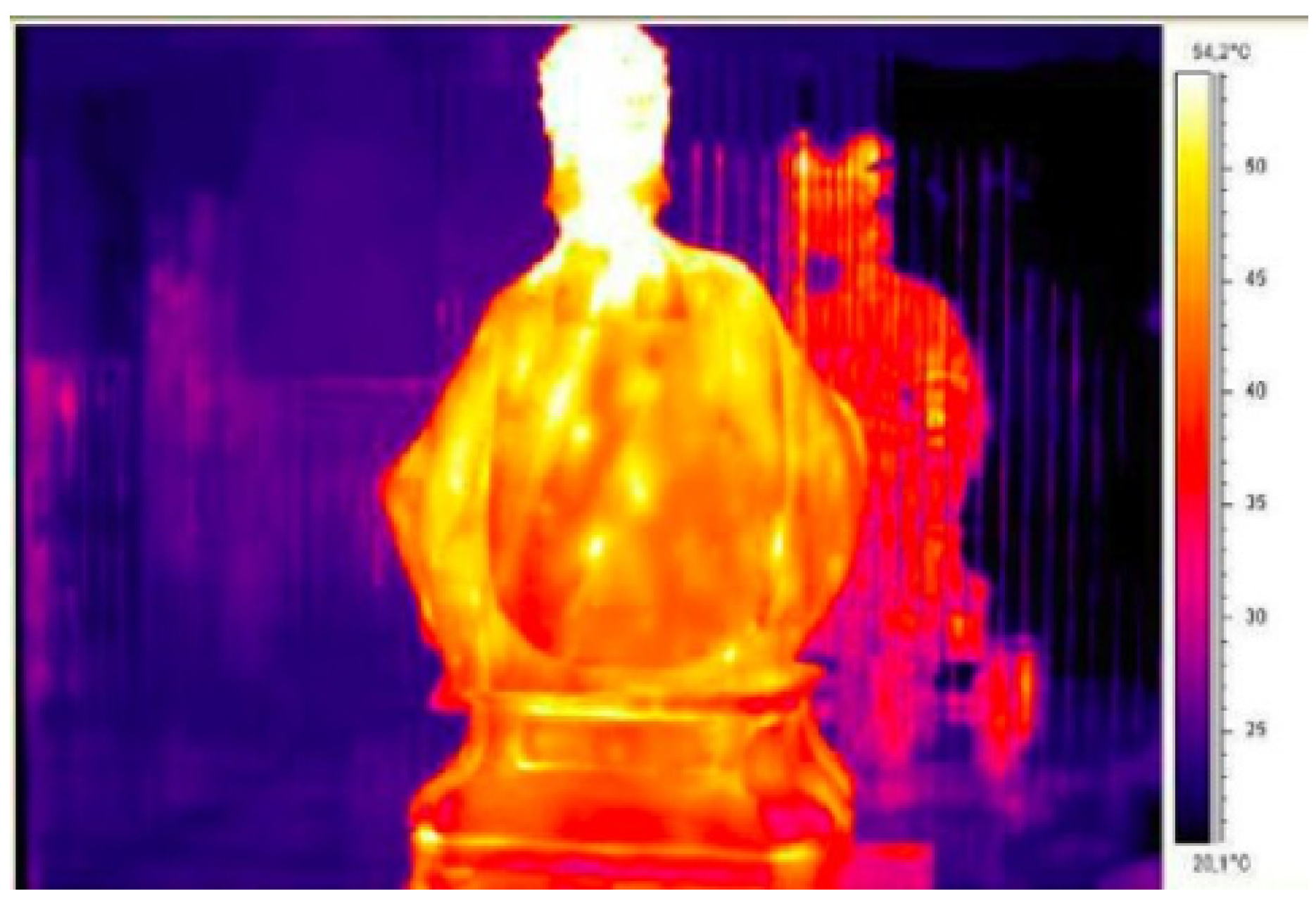
Besides the aforementioned methods, the microwave heating is a promising application for treatment of works of art [9]. As showed in our previous research, several laboratory exposures were conducted for the treatment of real works of art: in particular, a precious wooden statue, obtaining a complete disinfestation of pests [10], and archeological remains in the Paestum Archeological Site (South of Italy) [11] (Figure 1).
Similar approaches are known quite well in literature, like, for example, the work of Riminesi et al. [12]. The microwave treatment, even if compelling and promising, may present some negative aspects if not correctly performed; among the others, it is worthwhile to mention the presence of highly heated areas (e.g., hot spots) or areas with poor radiation as a consequence of particular shapes [5].
In this context, this paper outlines a prediction model, developed in order to envisage the distribution of heating power into the objects to be treated, even of complex shapes enabling one to define a priori the exposure time. The model can also predict the behavior of irradiation when the object is infested by other entities such as nails or pests. The data to be provided for performing a simulation are the geometry of the object (or objects in case one performs a multiple loading) and their dielectric characteristics. As a result, we obtain the distribution of heating power [13].
Given the above, it is clear that microwaves constitute a safe and effective methodology for this kind of treatment, although, in some situations, it will be necessary to carefully evaluate any unwanted effects [14]. For the evaluation of such effects, it is useful to proceed to the heating simulation, avoiding unwanted effects during the real treatment, this is significant for development of treatment procedure of important goods [15]. Several models reproduce the electromagnetic field in a reverberation chamber equipped with a mechanical mode stirrer, and some numerical results are compared with experimental measurements with a good agreement. Mode Stirred Reverberation Chambers (MSRC) guarantee a controlled electromagnetic environment around biological materials for exposure to electromagnetic fields [16,17].
The advantage of creating a model of the object for a faithful simulation of the reality is twofold; on the one hand, it is possible to determine the presence of areas not hot enough to ensure the effectiveness of the disinfectant treatment. On the other hand, one can predict if there are too hot zones in which irreparable damage of the good to be treated might occur [18]. Additionally, a second benefit of the simulation is to be able to determine the relationship between the temperature in the interior points to the object, and therefore inaccessible in practice, and the surface ones that are easily monitored even during the actual treatment. Thanks to these relationships, the evaluation of the temperature can be conducted at each point in real time, in order to ensure the effectiveness and safety of the treatment. Finally, another advantage of the simulation is to evaluate the possible resonances of biological agglomerates subject to the electromagnetic field; this effect could create an unexpected overheating condition that could seriously damage the treated good. The methodology and treatment protocol were developed according to laboratory tests, exposing some samples of different essences of wood into a reverberation chamber. We tested the microwave application in order to evaluate the management of disinfestations of wooden works, monitoring temperature and incident power [19,20]. Some samples were prepared to test the use of microwaves on wooden works of art. The samples were very similar to real artistic objects, both painted and not painted. We did not observe any significant modifications in the samples [5]. For this kind of treatment, 2.45 GHz ISM frequency is largely used. Other frequency values are not convenient for the power absorbed by the materials that normally constitute the cultural objects, while higher values are not suitable because of the low penetrating power of electromagnetic fields. Preliminary results showed that the treatment is optimized for wood samples in the temperature range 50 T 60 C [10]. It is well known that our cultural heritage ranges among countless typology of works: wood (furniture, frames, musical instruments, etc.), paper (books, documents, etc.) [21], cloth (carpets, tapestries, canvas, etc.), which are generally subjected to the attack of bugs (woodworms), moulds, and funguses [22,23].
The main contribution of the proposed methodology, in addition to those described, is that it could be extended to objects of historical-artistic interest made up of different materials, from very simple mono-components to complex structures integrating inorganic and organic matters.
The rest of the paper is organized as follows: the second section is devoted to the description of the methods and mathematical assumptions derived to postulate the model. In Section 3, the main results achieved are shown, while, in the last section, concluding remarks and future developments are presented.
2. Methods
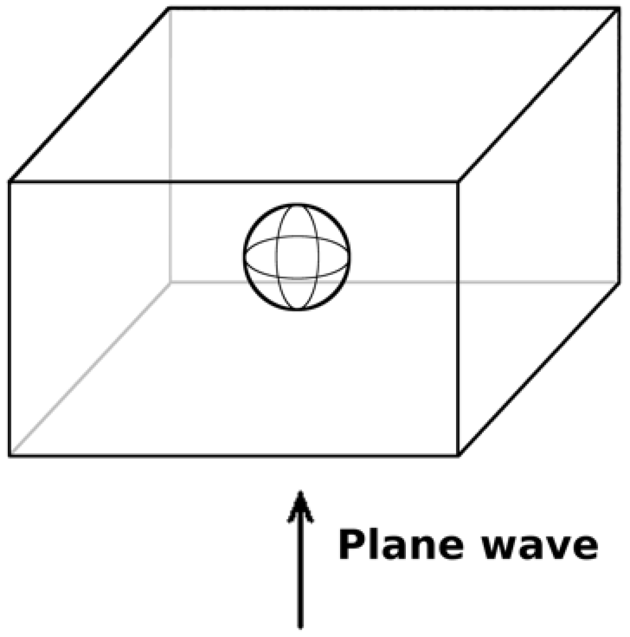
The resonances model study was developed from a strong theoretical base to make its application as wide as possible. This way was supplied by Mie [24] that introduced an exact solution of Maxwell equations, in order to estimate the electromagnetic field. Figure 2 shows a schematic of a block in the shape of parallelepiped with losses that contains a sphere of dielectric material with losses too, all invested by a plane wave [25,26,27]. In our specific case, the block is made of wood and the sphere is made of water. This choice is due to the dielectric characteristics of biological agents, infesting wooden artifacts, which is similar to water [28].
2.1. Derivation
The exact solution of the problem is obtained starting from the Maxwell equations by using the vectors potential, with the spherical symmetry, and expressing the plane wave as an infinite sum of spherical waves. There are two solutions: the fields around the sphere and those on the inside. For the continuity principle of the electric and magnetic field tangential components, on the surface of separation of the two domains, the two solutions have to get the same results. This condition allows the coefficients fields’ evaluation. By considering a spherical coordinate system and the mathematical expression of a plane wave, as shown in Figure 3, that proceeds along the direction of the z-axis with the field polarized in the x-axis:
where is the unit vector of the x-axis and is the angular wave number. The expression of plane waves in terms of spherical coordinates becomes:
where , are the three unit vectors of the three spherical coordinates in the exam. As clearly explained in [25], the field can be expressed with the resulting three expressions:
where arises from:
with spherical Bessel function, is Legendre Polynomials and where:
The electromagnetic field can be found by using the scalar Helmholtz equation:
The solution of this equation can be obtained with the method of separation of variables, and the functions that satisfy the solution can be expressed as:
The two previous expressions were combined and the Helmholtz equation was split into three new equations that are independent:
These three equations are respectively: the Bessel differential equation (its solutions are the Bessel functions); the Legendre differential equation (its solutions are given by Legendre polynomials); and the classical harmonic differential equation (its solutions are sinusoidal functions). From Equation (9), it is possible derive the expressions of potential vectors A and F [26]; in this case, they have only one component different from zero: this component is the unit vector along the radial.
Their expressions slightly vary according to the incident field:
with:
or scattered field:
with obtained from the spherical Hankel functions of the second kind according with the expression:
The Hankel functions of the second kind replace the Bessel equations. In fact, the Bessel equations accept the argument equals zero, which is necessary in this circumstance, because it represents the center of the sphere. In the last two expressions, the coefficients and should be defined, while is the characteristic impedance of the block that contains the sphere. The total field, sum of incident and scattered fields will depend on the sum of the two contributions:
The values of E and H derive from and from applying the expressions:
where and are, respectively, the magnetic permeability and the magnetic permittivity of the block. The potential vectors are defined by the following expressions:
where the d index indicates that the values are referred to the sphere material. At this point, in order to obtain the final expression for the fields’ evaluation, it is necessary to determine the coefficients , , and . For this purpose, it is assuming, in the surface of the sphere, the continuity of the tangential components of the fields, and it is pointing with the t index to the total fields outside the sphere and with the d index to those within and for :
By replacing the expressions for A and F, the final expressions are obtained. However, the incident field is given by the plane wave that invests the sphere. For the diffused fields outside the sphere:
The scattered fields, obtained with the coordinate transformation, are added to the previous ones. Then, the results are:
where the coefficients are:
For fields inside the sphere:
In the above expressions, the coefficients have the following values:
with the constants , , and , and the d index indicates that the parameter is related to the material of the sphere, while the absence of an index indicates that it is related to the block.
, , and respectively indicate:
The previous expressions can be encoded with any programming language (Fortran, Pascal, C, Matlab, Mathematics, etc.) for the values evaluation of the electromagnetic field in all points of the sphere and the surrounding space. The result obtained is not satisfactory from the point of view of the study of irradiation and distribution of density power because it has an asymmetrical situation. This situation is given by the plane wave from a well-defined direction (z-axis). By summing the fields from the same model with the change of the direction of the plane wave and its direction of propagation, a situation more adherent to what occurs in a reverberation chamber is obtained. By considering three axes, the two ways of propagation, there are a total of six plane waves.
2.2. Numerical Model Study
Microwave heating is a well-established practice in the conservation of the works of art. In many situations, when the object that must be treated is valuable, it may be useful to predict the behaviour of the reverberation chamber, in order to avoid its damage and the presence of hot spots for particular dimensions of pests. The hot spots are points that are very hot in which overheating of the material occurs. It is necessary to investigate the possibility of the occurrence these situations. The simulation consists in the study of the microwave heating of pests, which are equivalent to a sphere of water, surrounded by a block of wood invested by six plane waves.
Table 1 lists the dielectric characteristics of the materials used in this study. Making the average of power density absorbed from waves coming from several directions, a peak corresponding to a sphere radius equal to 6.84 mm was observed. This measure is close to half the electromagnetic field wavelength of the sphere. The electromagnetic field wavelength is:
where is the velocity and f the frequency.
Furthermore,
and permeability of free space, and , with permittivity of free space and relative permittivity of water.
2.3. Experimental Study
The resonance peak occurs for R = 6.84 mm, and we define mm. The situation was also evaluated in two other points, before the resonance with and after the resonance with .
We will therefore examine three different cases:
- At the resonance Radius = = 6.84 mm,
- Out of resonance Radius = 5.42 mm < ,
- Out of resonance Radius = 8.13 mm > ,
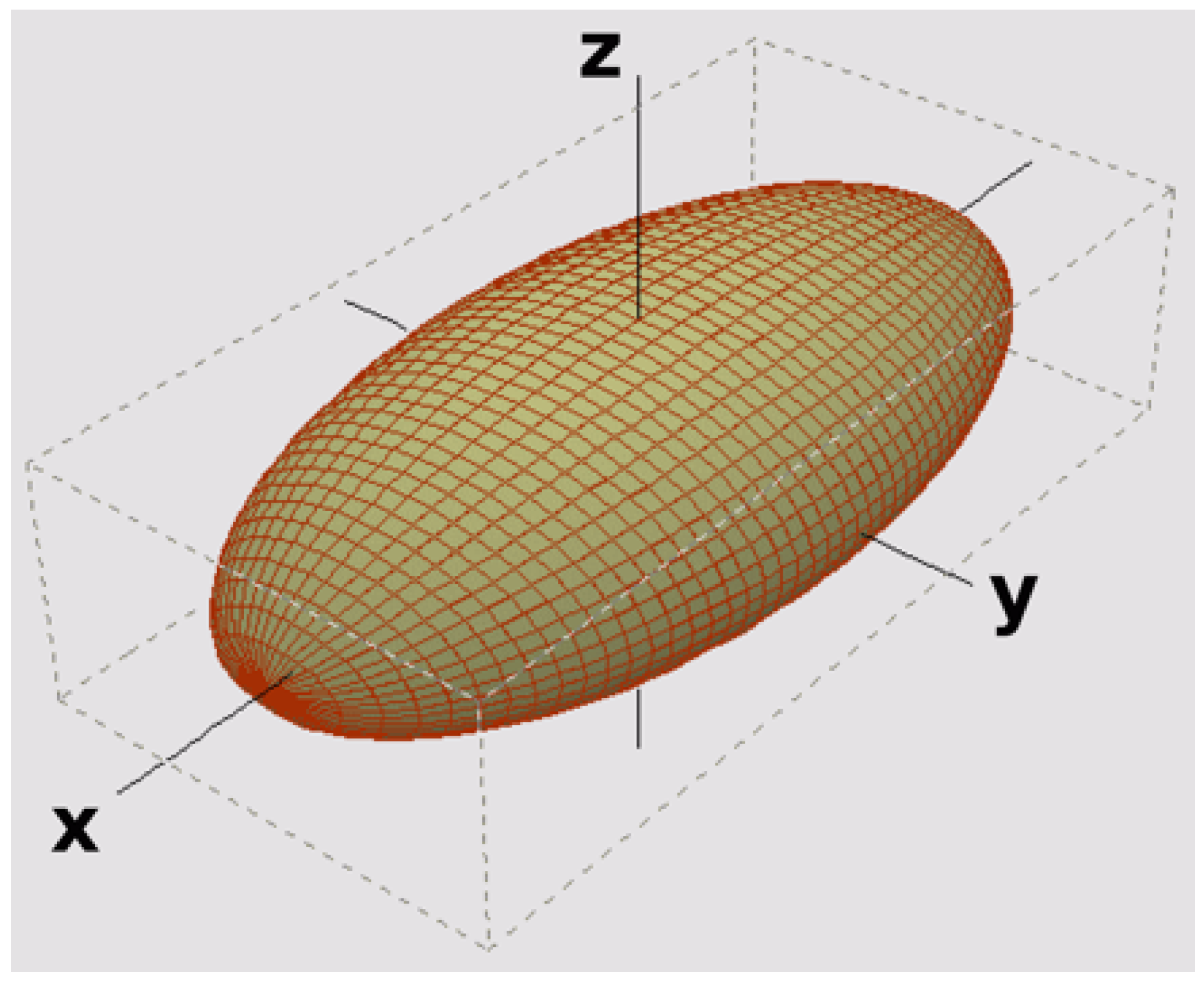
where the values of the rays 5.42 mm and 8.13 mm were chosen considering +20% and −20% from the radius in which it has observed the resonance. For a better adherence to reality, the model of the biological organism has been generalized to a prolate ellipsoid (Figure 4), which is a model with a longer semi-major axis (which will be indicated with a) and the other two shorter and identical axes (indicated by b and c that satisfy the equality and then b = c); in addition, to reduce the degrees of freedom, a = 5b has been set to ensure that the appearance is somewhat oblong and resembling the most common weed species.
Although is possible to choose a theoretical study of the exact problem [29], and also empirical [30], this paper deals the case-level simulation. The processing cycle was performed by the program COMSOL, both for the electromagnetic part that for the thermal. In particular, as regards the electromagnetic aspect, there were simulated four plane waves coming from perpendicular directions to the major axis of the ellipsoid, having all of polarization along that axis. The plane waves come from y+, y−, z+, and z− directions all with polarization along the x-axis, which is the one parallel to the major axis of the ellipsoid. As in the case of sphere, the simulations are performed varying the semimajor axis a.
In this case, the three different cases are the following:
- At the resonance with a = 16.69 mm and b = 3.34 mm;
- Out of resonance with a = 26.71 mm and b = 5.34 mm;
- Out of resonance with a = 8.68 mm and b = 1.74 mm.
3. Results and Discussion
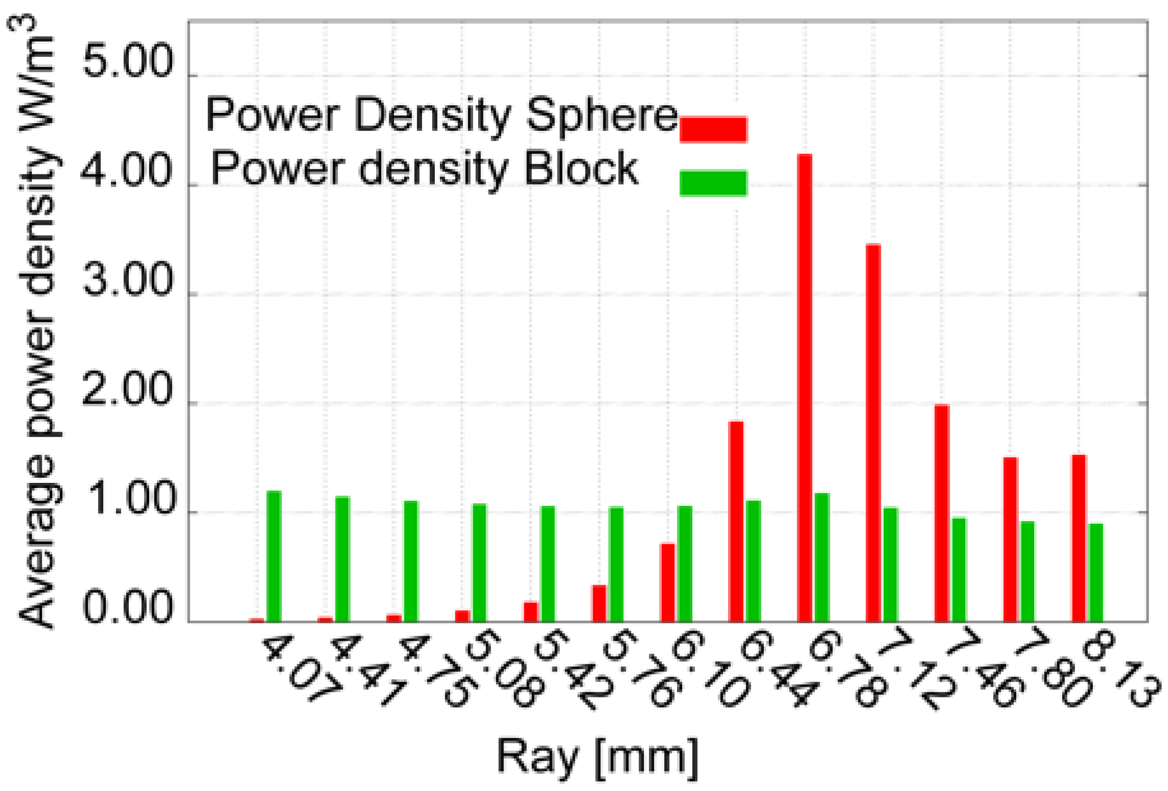
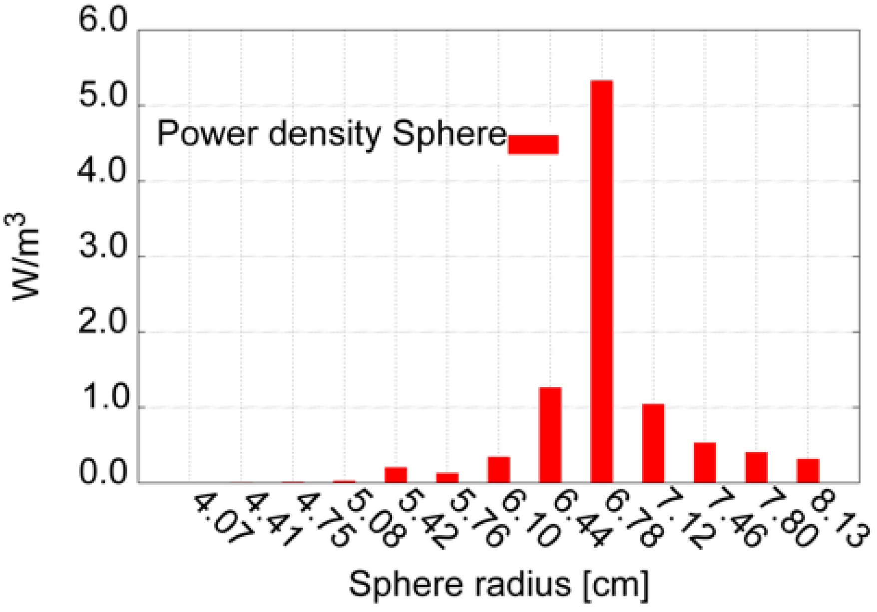
Figure 5 reports the histogram of the average power density absorbed by the sphere compared with the power density absorbed by the block, for radius values near the resonance with increments or decrements of 5%.
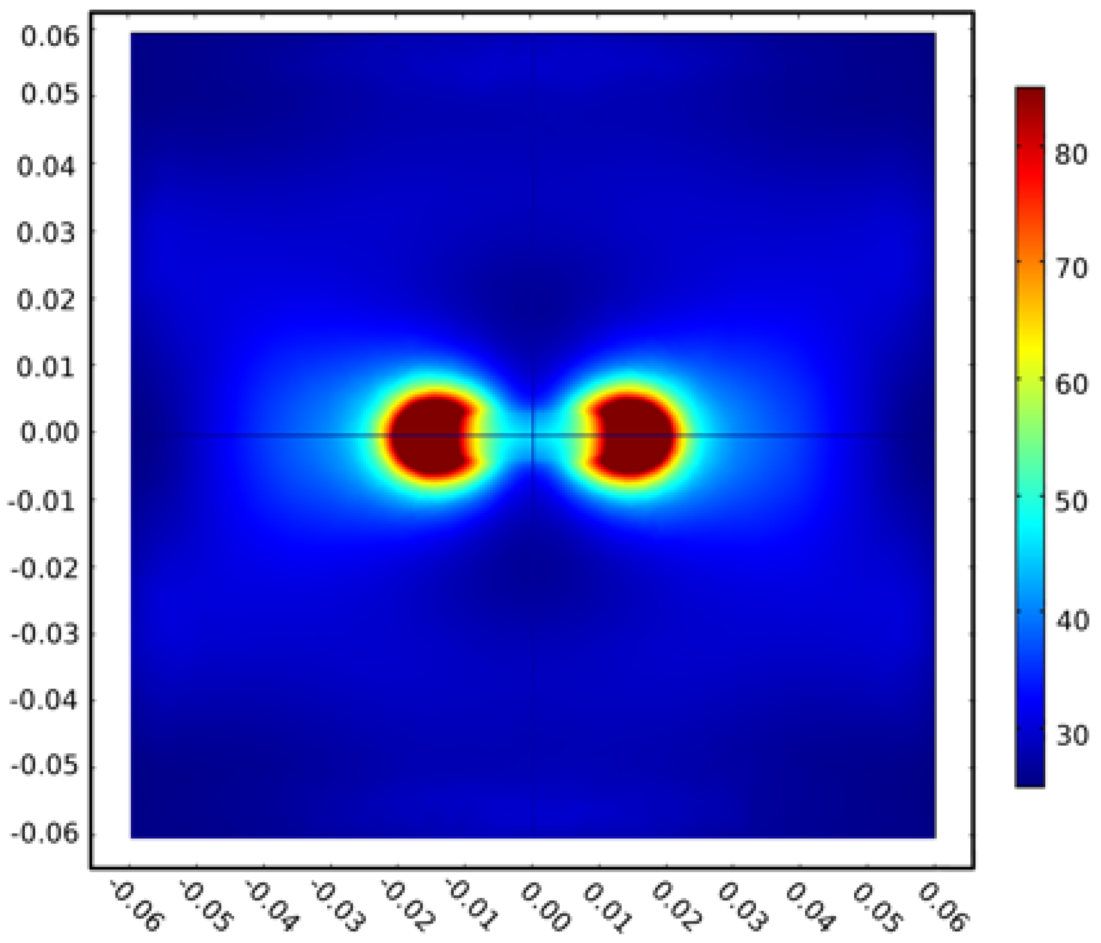
The variability of the average power density absorbed by the sphere to the change of its radius can be noted immediately. Instead, the power density absorbed by the block of wood remains constant. With the power density map obtained, it was possible to represent the thermal simulation. The temperature visualization in a transversal plane to the block and passing for its center (cutting the sphere), in addition to the vertical axis, was particularly significant. The first representation is Figure 6, which displays the temperatures in the form of colors. The second representation in Figure 7, which is more precise, consists of a Cartesian graphic that describes the temperature along a central axis.
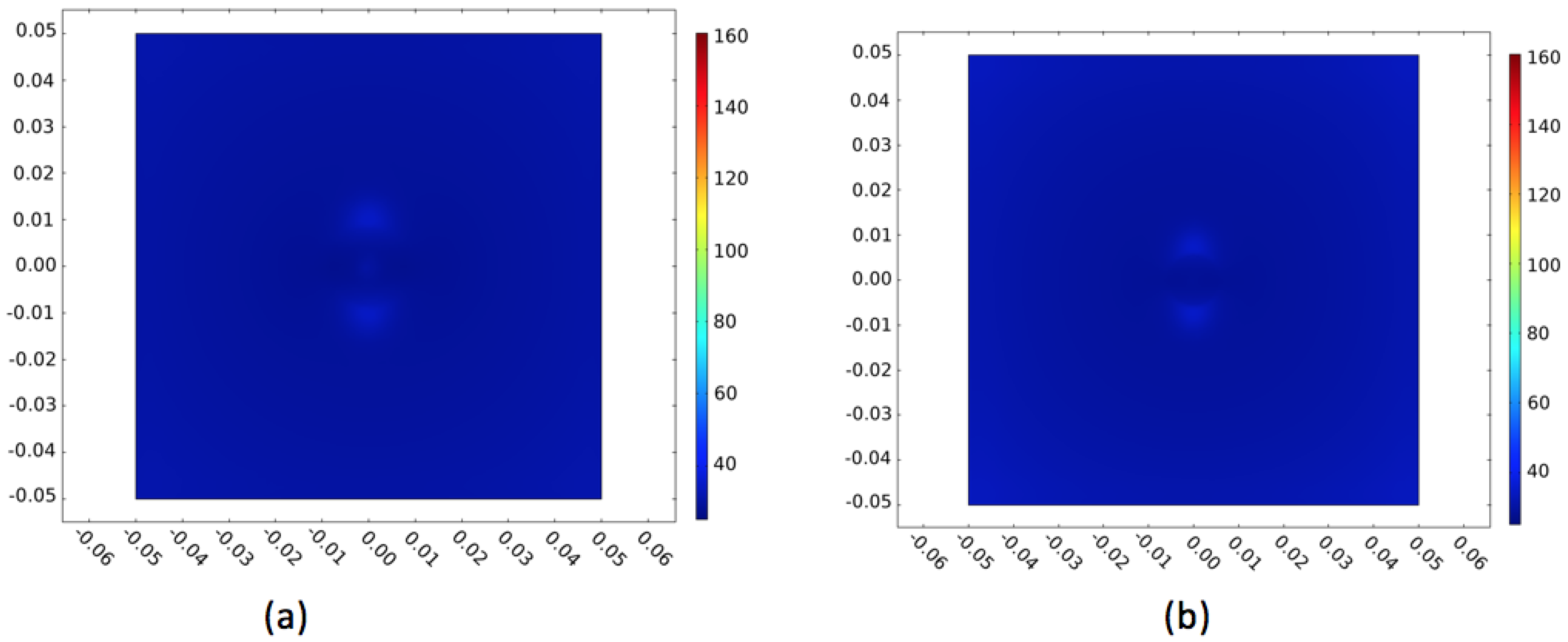
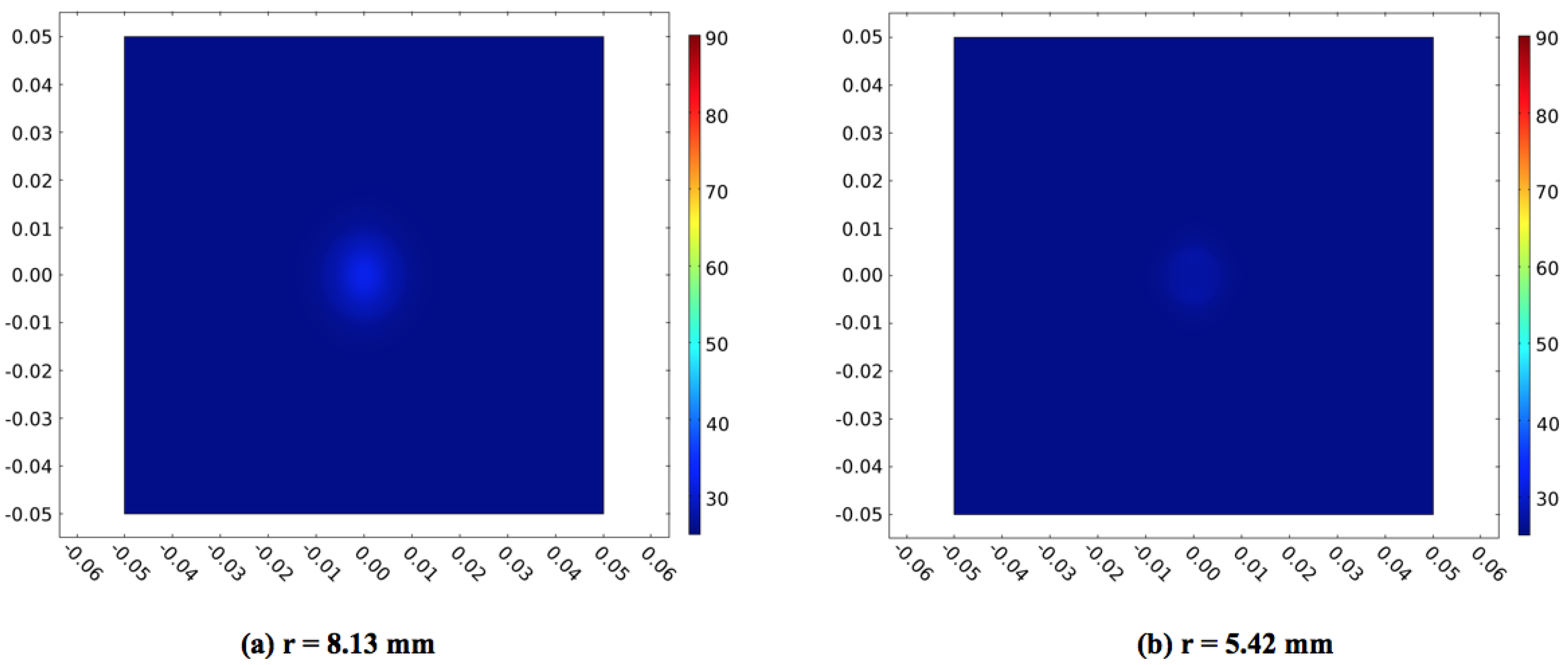
The initial temperature was 25 C and the heating was for 60 s for the dimension of the sphere with a radius equal to mm. In this case, an average increase of temperature of 5 C in the block was observed, while, in the sphere, the increase was over 130 C. In this condition, part of the sphere heat will warm the surrounding wood. The other two conditions take Radius = 5.42 mm < and Radius = 8.13 mm > Rris (Surface maps: Figure 8; Temperature diagrams (Figure 9)) with a heating uniformity in the whole block can be noticed, with a temperature lower in the center of the sphere. In this point, the surrounding wood will warm the sphere.
The heat flux wood-sphere depends on the sphere dimension. In case of fir wood, the behaviour is the same, even a decrease of wood heat for its low conductibility could be noticed (Figure 10).
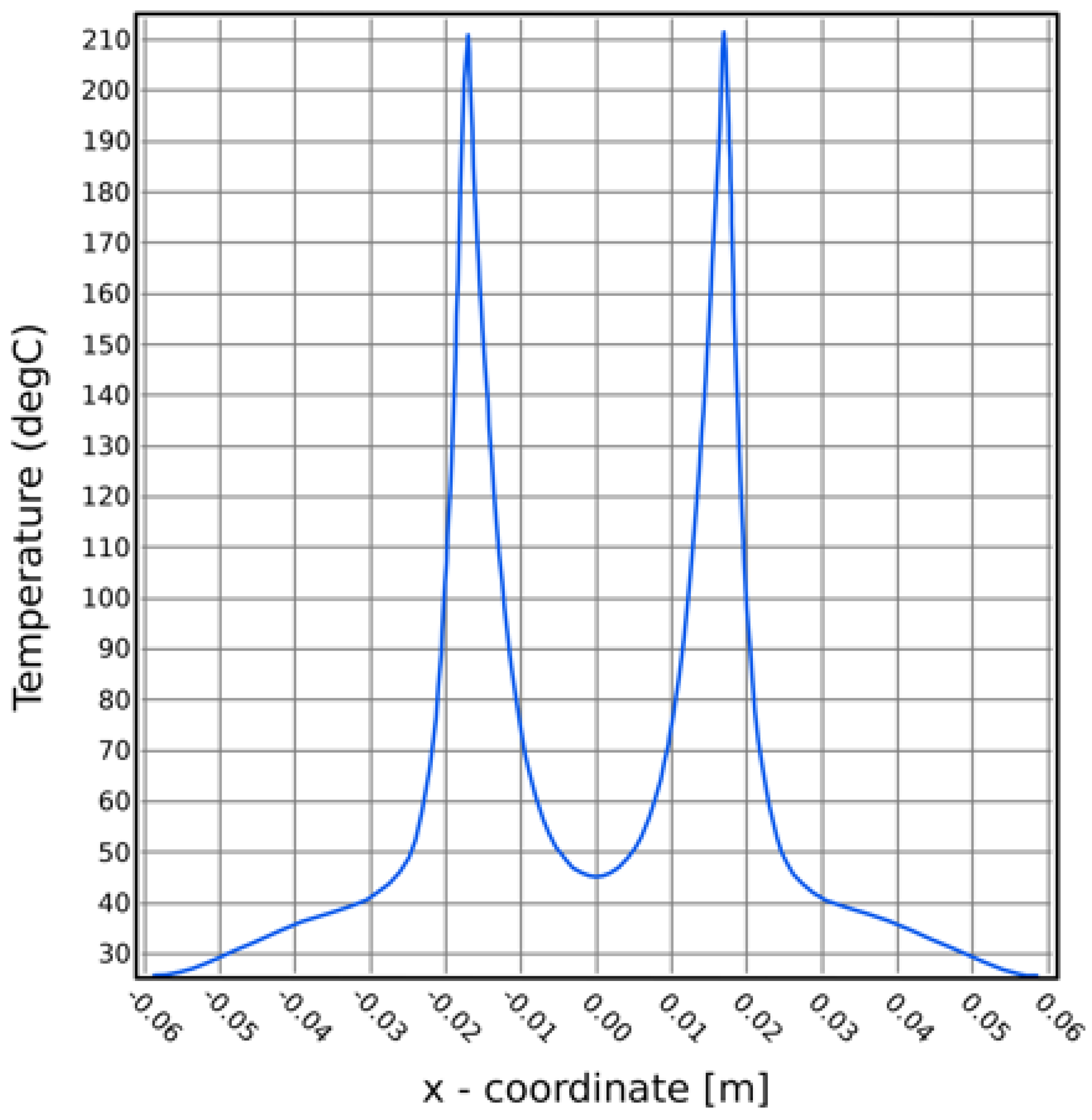
For an equal time treatment, the wood remained at the starting temperature, the sphere, instead, warms in case of resonance. Figure 11 and Figure 12 depict the graphics in the resonance case.
4. Conclusions and Future Works
Works of art are an important national wealth for each country. Therefore, they should be protected and preserved by all the possible causes of damage. Dealing with wooden artifacts, a significant cause of damage is made by the pests that can erode the structure.
The presence of biological organisms in the works of art can be extremely dangerous for their preservation; however, treatments of disinfection, by means of microwaves, can lead to problems of permanent damage if their dimensions and characteristics are such that they will bring to the resonance frequency of the pests.
The proposed methodology is useful to calculate the response of biological materials subject to microwave exposure and to prevent the risk of resonance. In fact, peak of resonance, as well as localized overheating, may cause irreversible damage to the good. The numerical model described in these pages has been applied to different shapes (both spherical and ellipsoidal) in order to better fit with the reality. However, even if the model has proved to be affordable to predict the heating behaviour, a preliminary diagnosis is mandatory in order to know in advance the characteristics and the model parameters. This is because their prediction is not easily implemented, mainly due to the uncertainty of these events. In these situations, it is desirable to be sure that the process is effective, but not risky for the integrity of the goods. Consequently, it is mandatory to investigate a priori the possible presence of these harmful conditions using techniques of experimental investigations such as nuclear magnetic resonance, axial tomography, and X-rays; in addition this, the study of possible pests species, size and their dielectric properties, in all the forms in which they can aggregate, is fundamental.
To date, MW treatments proved to be a valuable method, and the possibility to know in advance the effects of the treatment opens up an interesting research path. Notwithstanding, no data are available in order to standardize the model and extend it to every object, or pests. Because of this, forthcoming investigations will be conducted by conservationists, archeologists and Art Historians in order to effectively validate the model with laboratory tests. Further efforts will be also dedicated to explore how different complex shapes of the object can influence the heating distribution. Moreover, thanks to this model, we will develop an application that simulates the heating of an object in a reverberation chamber. This application makes it easy for non-electromagnetic personnel to employ the mathematical models, it can visualise the distribution of temperature in objects to be treated and it is possible to insert the power to be transmitted in the chamber [28].
Author Contributions
Introduction, M.P., R.P. and E.F.; methods R.B., M.P., B.B. and R.D.; Results, R.P., R.B., M.P., B.B. and R.D.; Discussion and Conclusion, R.P., R.B., M.P., E.F., B.B. and R.D. All the authors contributed to the development and set up of the general idea.
Funding
This research received no external funding.
Conflicts of Interest
The authors declare no conflict of interest.
References
- Sutter, G.; Sperlich, T.; Worts, D.; Rivard, R.; Teather, L. Fostering cultures of sustainability through community-engaged museums: The history and re-emergence of ecomuseums in Canada and the USA. Sustainability 2016, 8, 1310. [Google Scholar] [CrossRef]
- Wesson, C. Rumors of Our Demise Have Been Greatly Exaggerated: Archaeological Perspectives on Culture and Sustainability. Sustainability 2013, 5, 100–122. [Google Scholar] [CrossRef]
- Lee, C.H.; Chen, H.S.; Liou, G.B.; Tsai, B.K.; Hsieh, C.M. Evaluating International Tourists’ Perceptions on Cultural Distance and Recreation Demand. Sustainability 2018, 10, 4360. [Google Scholar] [CrossRef]
- Crova, C.; Chiadini, F.; Di Maio, L.; Guerriero, L.; Pescione, L. Elimination of Xylophages from Wood through Microwave Treatment: Microstructural Experiments. Conserv. Sci. Cult. Herit. 2018, 17, 45–57. [Google Scholar]
- Pia Pastore, A.; Bisceglia, B.; De Leo, R.; Diaferia, N. An innovative microwave system for wooden art object disinfestation. COMPEL Int. J. Comput. Math. Electr. Electron. Eng. 2012, 31, 1173–1177. [Google Scholar] [CrossRef]
- Casieri, C.; Senni, L.; Romagnoli, M.; Santamaria, U.; De Luca, F. Determination of moisture fraction in wood by mobile NMR device. J. Magn. Resonance 2004, 171, 364–372. [Google Scholar] [CrossRef] [PubMed]
- van der Werf, I.D.; Gnisci, R.; Marano, D.; De Benedetto, G.E.; Laviano, R.; Pellerano, D.; Vona, F.; Pellegrino, F.; Andriani, E.; Catalano, I.M.; et al. San Francesco d’Assisi (Apulia, South Italy): Study of a manipulated 13th century panel painting by complementary diagnostic techniques. J. Cult. Herit. 2008, 9, 162–171. [Google Scholar] [CrossRef]
- Mascalchi, M.; Osticioli, I.; Riminesi, C.; Cuzman, O.A.; Salvadori, B.; Siano, S. Preliminary investigation of combined laser and microwave treatment for stone biodeterioration. Stud. Conserv. 2015, 60, S19–S27. [Google Scholar] [CrossRef]
- Olmi, R.; Bini, M.; Ignesti, A. Investigation of the Microwave Heating Method for the Control of Biodeteriogens on Cultural Heritage Assets In. In Proceedings of the 10th International Conference on Non-Destructive Investigations and Microanalysis for the Diagnostics and Conservation of Cultural and Environmental Heritage, Florence, Italy, 13–15 April 2011. [Google Scholar]
- Bisceglia, B.; Diaferia, N.; Acquaro, M. MW treatment of wooden handicrafts. The restoration of San Leone Magno statue. In Proceedings of the 30th Bioelectromagnetics Society Annual Meeting, San Diego, CA, USA, 8–12 June 2008. [Google Scholar]
- Bacchiani, R.; Bisceglia, B.; De Leo, R. Industrial Applications of Microwaves: Cultural Heritage Conservation. In Proceedings of the ICEMB Interazioni fra Campi Elettromagnetici e Biosistemi, Bologna, Italy, 27–29 June 2012; pp. 27–29. [Google Scholar]
- Riminesi, C.; Olmi, R. Localized microwave heating for controlling biodeteriogens on cultural heritage assets. Int. J. Conserv. Sci. 2016, 7, 281–294. [Google Scholar]
- Bacchiani, R.; Bisceglia, B.; De Leo, R. Microwave treatment of biological systems: Simulation of heating in reverberating chamber. In Proceedings of the International Conference Bio & Food Electrotechnologies (BFE 2012), Salerno, Italy, 26–28 September 2012; pp. 26–28. [Google Scholar]
- Serra, R.; Canavero, F. Linking a one-dimensional reverberation chamber model with real reverberation chambers. In Proceedings of the 2008 International Symposium on Electromagnetic Compatibility-EMC Europe, Hamburg, Germany, 8–12 September 2008; pp. 1–6. [Google Scholar]
- Bisceglia, B.; De Leo, R.; Pastore, A.P.; von Gratowski, S.; Meriakri, V. Innovative systems for cultural heritage conservation. Millimeter wave application for non-invasive monitoring and treatment of works of art. J. Microw. Power Electromagn. Energy 2011, 45, 36–48. [Google Scholar] [CrossRef]
- Andrieu, G.; Soltane, A.; Reineix, A. Analytical model of a mechanically stirred reverberation chamber based on EM field modal expansion. In Proceedings of the 2016 International Symposium on Electromagnetic Compatibility-EMC EUROPE, Wroclaw, Poland, 5–9 September 2016; pp. 217–222. [Google Scholar]
- Lallechere, S.; Girard, S.; Roux, D.; Bonnet, P.; Paladian, F.; Vian, A. Mode stirred reverberation chamber (MSRC): A large and efficient tool to lead high frequency bioelectromagnetic in vitro experimentation. Prog. Electromagn. Res. 2010, 26, 257–290. [Google Scholar] [CrossRef]
- Ma, L.; Paul, D.L.; Pothecary, N.; Railton, C.; Bows, J.; Barratt, L.; Mullin, J.; Simons, D. Experimental validation of a combined electromagnetic and thermal FDTD model of a microwave heating process. IEEE Trans. Microw. Theory Tech. 1995, 43, 2565–2572. [Google Scholar]
- De Leo, R.; Russo, P.; Scalise, L.; Tomasini, E. Temperature monitoring by infrared techniques into RF ovens. In Proceedings of the International Conference on Microwave and High Frequency Heating, Fermo, Italy, 9–13 September 1997; pp. 433–436. [Google Scholar]
- Chidichimo, G.; Dalena, F.; Beneduci, A. Woodworm Disinfestation of Wooden Artifacts by Vacuum Techniques. Conserv. Sci. Cult. Herit. 2015, 15, 267–280. [Google Scholar]
- Calò, G.; D’Orazio, A.; De Sario, M.; Mescia, L.; Petruzzelli, V.; Prudenzano, F. Analysis of microwave thermal treatment of antique books with metallic insets. J. Microw. Power Electromagn. Energy 2007, 42, 48–60. [Google Scholar] [CrossRef]
- Andreueeetti, D.; Bini, M.; Ignesti, A.; Gambetta, A.; Olani, R. Microwave destruction of woodworms. J. Microw. Power Electromagn. Energy 1994, 29, 153–160. [Google Scholar] [CrossRef]
- Augelli, F.; Bisceglia, B.; Boriani, M.; Diaferia, N.; Foppiani, F.; Italiano, E.; Magli, F.; Mastropirro, R.; Tessari, R. Microwave Treatment of wood artistic samples. Exposure of wooden handicrafts. In Proceedings of the 29th Bioelectromagnetics Society Annual Meeting, Kanazawa, Japan, 10–15 June 2007; pp. 11–15. [Google Scholar]
- Mie, G. Beiträge zur Optik trüber Medien, speziell kolloidaler Metallösungen. Annalen der Physik 1908, 330, 377–445. [Google Scholar] [CrossRef]
- Harrington, R.F. Fields, Time-Harmonic Electromagnetic Fields; IEEE Press: New York, NY, USA, 2001. [Google Scholar]
- Balanis, C.A. Advanced Engineering Electromagnetics; John Wiley & Sons: Hoboken, NJ, USA, 1999. [Google Scholar]
- Fall, A.K.; Besnier, P.; Lemoine, C.; Zhadobov, M.; Sauleau, R. Experimental dosimetry in a mode-stirred reverberation chamber in the 60-GHz band. IEEE Trans. Electromagn. Compat. 2016, 58, 981–992. [Google Scholar] [CrossRef]
- Paolanti, M.; Pollini, R.; Frontoni, E.; Mancini, A.; De Leo, R.; Zingaretti, P.; Bisceglia, B. Exposure protocol setup for agro food treatment. Method and system for developing an application for heating in reverberation chamber. In Proceedings of the 2015 IEEE 15th Mediterranean Microwave Symposium (MMS), Lecce, Italy, 30 November–2 December 2015; pp. 1–4. [Google Scholar]
- Barber, P.W. Resonance electromagnetic absorption by nonspherical dielectric objects. IEEE Trans. Microw. Theory Tech. 1977, 25, 373–381. [Google Scholar] [CrossRef]
- Durney, C.; Iskander, M.; Massoudi, H.; Johnson, C. An empirical formula for broad-band SAR calculations of prolate spheroidal models of humans and animals. IEEE Trans. Microw. Theory Tech. 1979, 27, 758–763. [Google Scholar] [CrossRef]
Figure 1.
The statue of San Leone Magno after microwave exposure.

Figure 2.
Block with sphere.

Figure 3.
Coordinate system and plane wave.

Figure 4.
The prolate ellipsoid.

Figure 5.
The prolate ellipsoid.

Figure 6.
Temperature chart of an oak block transversal plane, which contains a water sphere with a resonance radius.
Figure 6.
Temperature chart of an oak block transversal plane, which contains a water sphere with a resonance radius.

Figure 7.
Diagram of the temperatures at the resonance radius.

Figure 8.
(a) temperature chart of an oak block transversal plane in which a water sphere out of resonance Radius = 8.13 mm is contained; (b) temperature chart of an oak block transversal plane in which a water sphere out of resonance Radius = 5.42 mm is contained.
Figure 8.
(a) temperature chart of an oak block transversal plane in which a water sphere out of resonance Radius = 8.13 mm is contained; (b) temperature chart of an oak block transversal plane in which a water sphere out of resonance Radius = 5.42 mm is contained.

Figure 9.
(a) diagram of the temperatures out of resonance Radius = 8.13 mm; (b) diagram of the temperatures out of resonance Radius = 5.42 mm.
Figure 9.
(a) diagram of the temperatures out of resonance Radius = 8.13 mm; (b) diagram of the temperatures out of resonance Radius = 5.42 mm.

Figure 10.
Average power density absorbed from fir wood block and from the sphere varying the radius around the resonance value with steps of 5%.
Figure 10.
Average power density absorbed from fir wood block and from the sphere varying the radius around the resonance value with steps of 5%.

Figure 11.
Temperature chart of a fir block transversal plane which contains a water sphere with a resonance radius.
Figure 11.
Temperature chart of a fir block transversal plane which contains a water sphere with a resonance radius.

Figure 12.
Diagram of the temperatures at the resonance radius.

Figure 13.
(a) temperature chart of a fir block transversal plane in which is contained a water sphere out of resonance Radius = 8.13 mm and (b) temperature chart of an oak block transversal plane which contains a water sphere out of resonance Radius = 5.42 mm.
Figure 13.
(a) temperature chart of a fir block transversal plane in which is contained a water sphere out of resonance Radius = 8.13 mm and (b) temperature chart of an oak block transversal plane which contains a water sphere out of resonance Radius = 5.42 mm.

Figure 14.
(a) diagram of the temperatures out of resonance Radius = 8.13 mm; (b) diagram of the temperatures out of resonance Radius = 5.42 mm.
Figure 14.
(a) diagram of the temperatures out of resonance Radius = 8.13 mm; (b) diagram of the temperatures out of resonance Radius = 5.42 mm.

Figure 15.
Temperature chart at resonance with a = 16.69 mm and b = 3.34 mm.

Figure 16.
Diagram of the temperatures at resonance.

Figure 17.
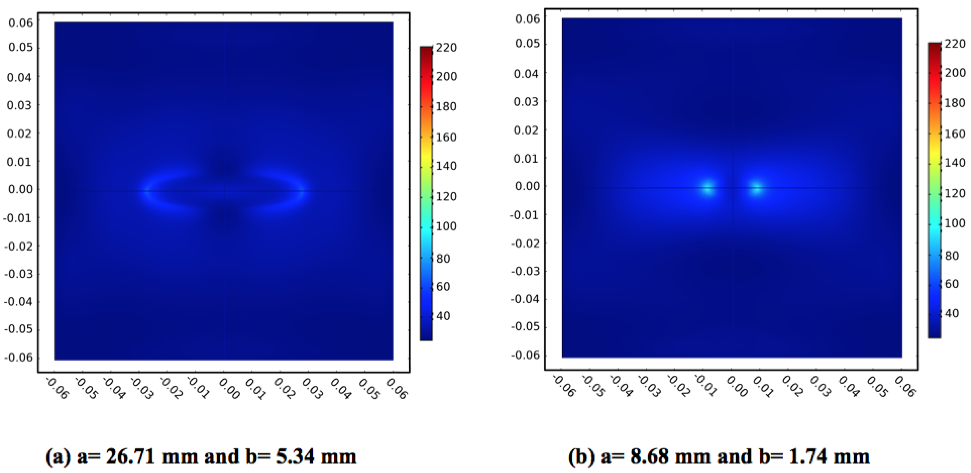
(a) temperature chart out resonance with a = 26.71 mm and b = 5.34 mm; (b) temperature chart out resonance with a = 8.68 mm and b = 1.74 mm.
Figure 17.
(a) temperature chart out resonance with a = 26.71 mm and b = 5.34 mm; (b) temperature chart out resonance with a = 8.68 mm and b = 1.74 mm.

Figure 18.
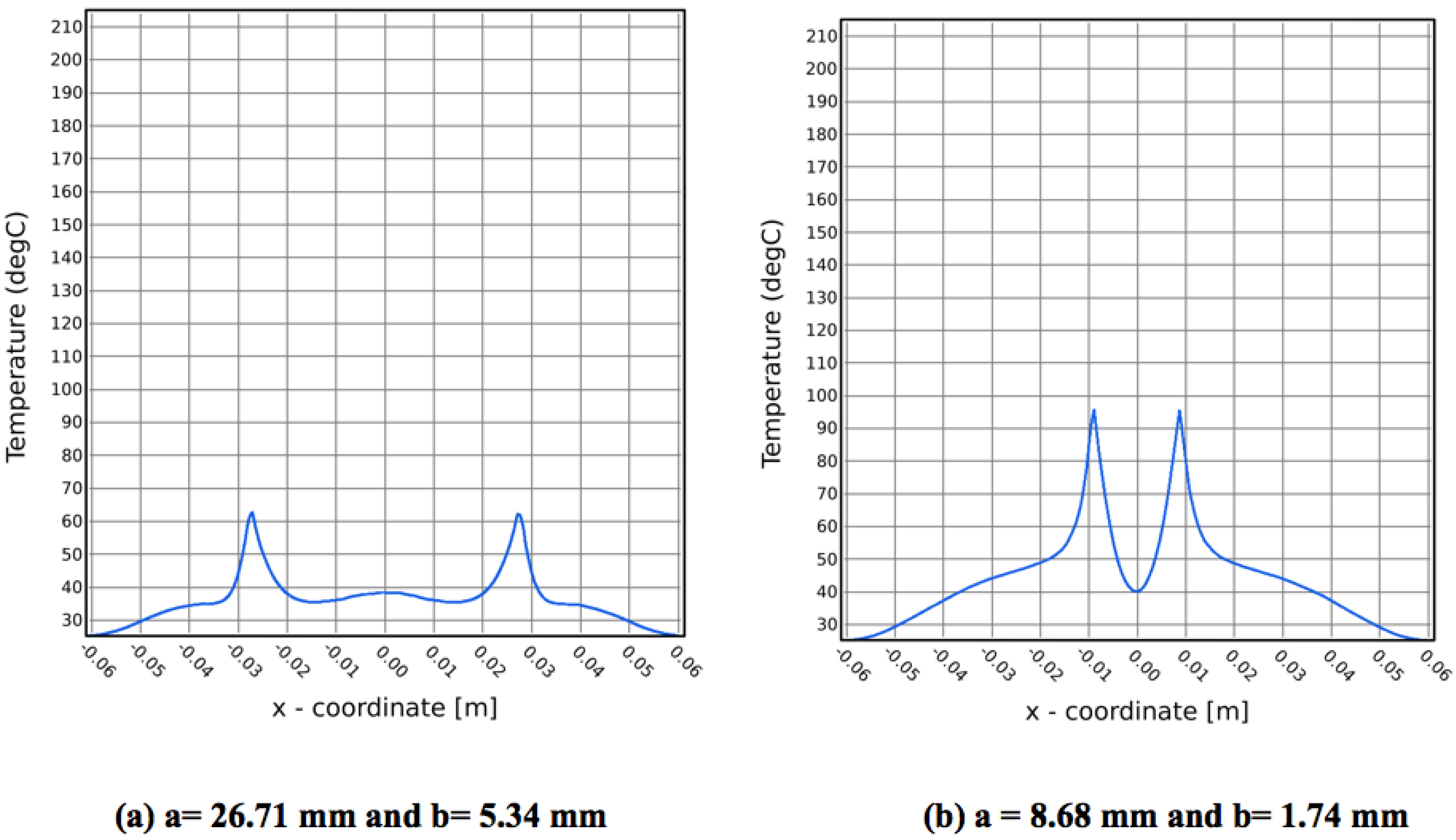
(a) diagram of the temperatures out of resonance with a = 26.71 mm and b = 5.34 mm; (b) diagram of the temperatures out of resonance with a = 8.68 mm and b = 1.74 mm.
Figure 18.
(a) diagram of the temperatures out of resonance with a = 26.71 mm and b = 5.34 mm; (b) diagram of the temperatures out of resonance with a = 8.68 mm and b = 1.74 mm.


Table 1.
Dielectric properties of the materials used in the scattering sphere simulation.
| Material | Relativity Permettivity | Conductivity | |
|---|---|---|---|
| Fir Wood | 1.82 | 0.0485 | 0.0066 |
| Oak Wood | 3 | 1.32 | 0.18 |
| Water | 80 | 5 | 0.681 |
© 2019 by the authors. Licensee MDPI, Basel, Switzerland. This article is an open access article distributed under the terms and conditions of the Creative Commons Attribution (CC BY) license (http://creativecommons.org/licenses/by/4.0/).
Share and Cite
MDPI and ACS Style
Pierdicca, R.; Paolanti, M.; Bacchiani, R.; de Leo, R.; Bisceglia, B.; Frontoni, E. Accurate Modeling of the Microwave Treatment of Works of Art. Sustainability 2019, 11, 1606. https://doi.org/10.3390/su11061606
AMA Style
Pierdicca R, Paolanti M, Bacchiani R, de Leo R, Bisceglia B, Frontoni E. Accurate Modeling of the Microwave Treatment of Works of Art. Sustainability. 2019; 11(6):1606. https://doi.org/10.3390/su11061606
Chicago/Turabian StylePierdicca, Roberto, Marina Paolanti, Roberto Bacchiani, Roberto de Leo, Bruno Bisceglia, and Emanuele Frontoni. 2019. "Accurate Modeling of the Microwave Treatment of Works of Art" Sustainability 11, no. 6: 1606. https://doi.org/10.3390/su11061606
Note that from the first issue of 2016, this journal uses article numbers instead of page numbers. See further details here.