Linking between Renewable Energy, CO2 Emissions, and Economic Growth: Challenges for Candidates and Potential Candidates for the EU Membership

 ,
,  , ,
, ,  ,
,  and
and
Abstract
:1. Introduction
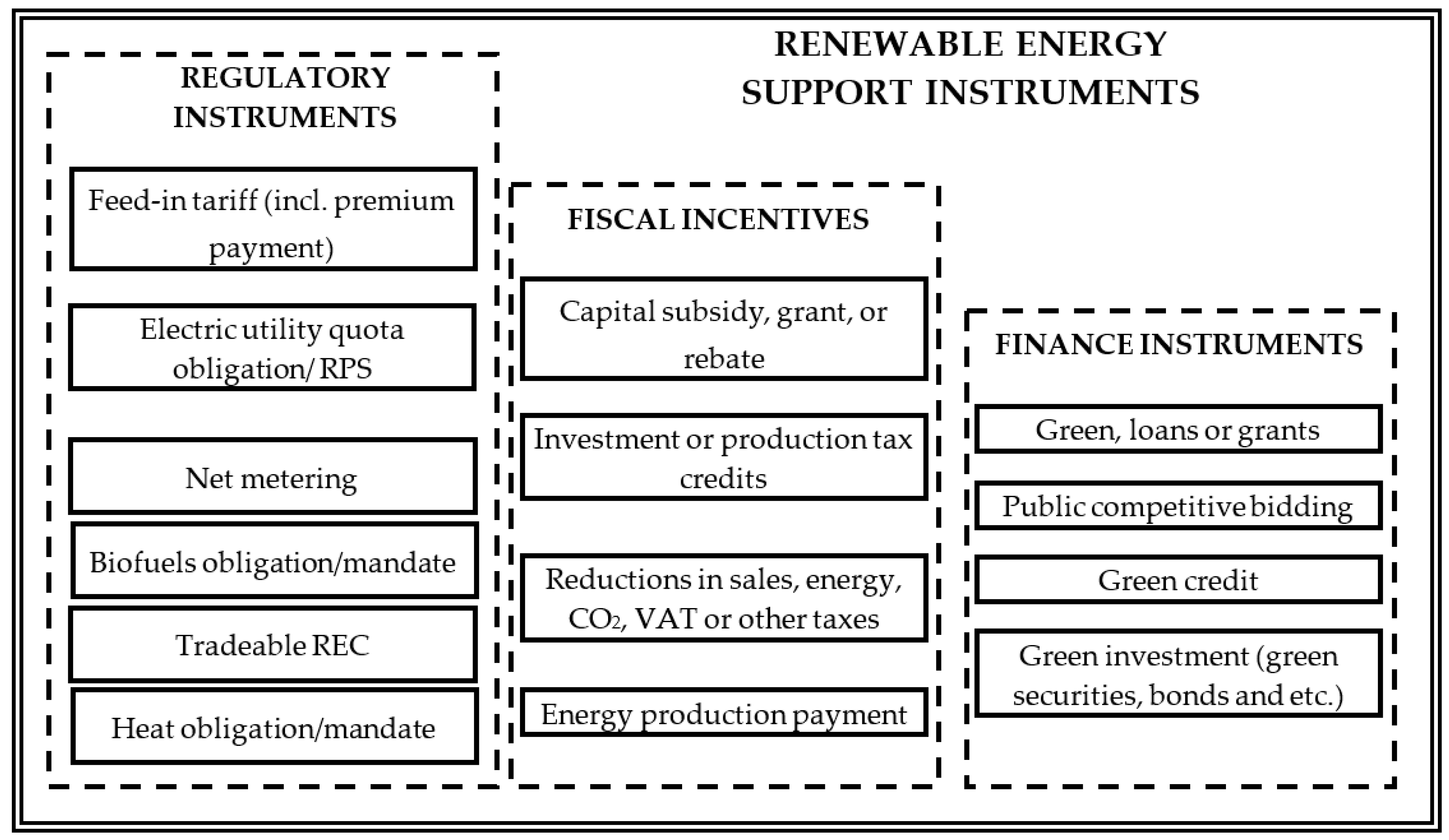
2. Methods
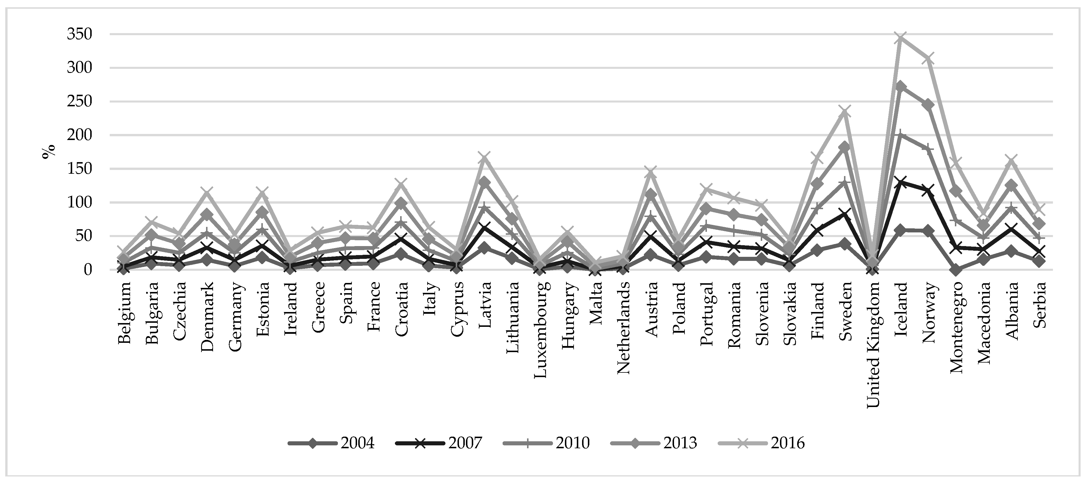
3. Results
4. Discussion
5. Conclusions
Author Contributions
Funding
Conflicts of Interest
References
- Conference of the Parties Twenty-First Session, P.3. (n.d.). Adoption of a Protocol, Another Legal Instrument, or an Agreed Outcome with Legal Force under the Convention Applicable to All Parties. Available online: http://unfccc.int/resource/docs/2015/cop21/eng/l09.pdf (accessed on 1 April 2016).
- Holthaus, E. Paris Agreement Ushers in End of the Fossil Fuel Era. 2016. Available online: http://www.slate.com/blogs/the_slatest/2015/12/12/paris_climate_agreement_will_lower_emissions_and_usher_in_end_of_the_fossil.html (accessed on 1 April 2016).
- European Environment Agency (EEA). Share of Renewable Energy in Gross Final Energy Consumption. 2018. Available online: https://ec.europa.eu/eurostat/tgm/table.do?tab=table&init=1&plugin=1&language=en&pcode=t2020_31 (accessed on 8 January 2019).
- Prokopenko, O.; Cebula, J.; Chayen, S.; Pimonenko, T. Wind energy in Israel, Poland and Ukraine: Features and opportunities. Int. J. Ecol. Dev. 2017, 32, 98–107. [Google Scholar]
- Sawin, J.L.; Sverrisson, F.; Seyboth, K.; Adib, R.; Murdock, H.E.; Lins, C.; Edwards, I.; Hullin, M.; Nguyen, L.H.; Prillianto, S.S.; et al. Renewables 2017 Global Status Report. 2017. Available online: https://inis.iaea.org/search/search.aspx?orig_q=RN:48058284 (accessed on 11 January 2019).
- World Development Indicators. Data Bank. Available online: http://databank.worldbank.org/data/reports.aspx?source=2&series=NY.GDP.MKTP.CD&country=UKR (accessed on 10 January 2019).
- CO2 Time Series 1990–2015 per Region/Country. Available online: http://edgar.jrc.ec.europa.eu/overview.php?v=CO2ts1990-2015&sort=des9 (accessed on 11 January 2019).
- Pimonenko, T.; Lyulyov, O.; Chygryn, O.; Palienko, M. Environmental Performance Index: Relation between social and economic welfare of the countries. Environ. Econ. 2018, 9, 1–11. [Google Scholar] [CrossRef]
- Vasylieva, T.; Lyeonov, S.; Lyulyov, O.; Kyrychenko, K. Macroeconomic stability and its impact on the economic growth of the country. Monten. J. Econ. 2018, 14, 159–170. [Google Scholar] [CrossRef]
- Kuznets, S. Economic growth and income inequality. Am. Econ. Rev. 1955, 45, 1–28. [Google Scholar]
- Bilgili, F.; Ozturk, I. Biomass energy and economic growth nexus in G7 countries: Evidence from dynamic panel data. Renew. Sustain. Energy Rev. 2015, 49, 132–138. [Google Scholar] [CrossRef]
- Bhandari, M.P. Impact of Tourism of off Road Driving on Vegetation Biomass, a Case Study of Masai Mara National Reserve, Narok, Kenya. Socio Econ. Chall. 2018, 3, 6–25. [Google Scholar] [CrossRef]
- Cebula, J.; Pimonenko, T. Comparison financing conditions of the development biogas sector in Poland and Ukraine. Int. J. Ecol. Dev. 2015, 30, 20–30. [Google Scholar]
- Lyulyov, O.; Chortok, Y.; Pimonenko, T.; Borovik, O. Ecological and economic evaluation of transport system functioning according to the territory sustainable development. Int. J. Ecol. Dev. 2015, 30, 1–10. [Google Scholar]
- Mačaitytė, I.; Virbašiūtė, G. Volkswagen Emission Scandal and Corporate Social Responsibility—A Case Study. Bus. Ethics Leadersh. 2018, 2, 6–13. [Google Scholar] [CrossRef]
- Pimonenko, T.; Prokopenko, O.; Dado, J. Net zero house: EU experience in Ukrainian conditions. Int. J. Ecol. Econ. Stat. 2017, 38, 46–57. [Google Scholar]
- Vasilyeva, T.; Lyeonov, S.; Adamičková, I.; Bagmet, K. Institutional quality of social sector: The essence and measurements. Econ. Sociol. 2018, 11, 248–262. [Google Scholar] [CrossRef]
- Directive, C. 70/220/EEC of 20 March 1970 on the Approximation of the Laws of the Member States Relating to Measures to Be Taken against Air Pollution by Gases from Positive-Ignition Engines of Motor Vehicles. OJ L076, 6, 1970. Available online: https://eur-lex.europa.eu/legal-content/EN/TXT/?uri=CELEX:31970L0220 (accessed on 11 January 2019).
- Chygryn, O. The mechanism of the resource-saving activity at joint stock companies: The theory and implementation features. Int. J. Ecol. Dev. 2016, 31, 42–59. [Google Scholar]
- Šincāns, E.; Ignatjeva, S.; Tvaronavičienė, M. Issues of Latvian Energy Supply Security: Evaluation of Criminal Offences in Latvia’s Electricity Market. Econ. Sociol. 2016, 9, 322–335. [Google Scholar] [CrossRef] [Green Version]
- Masharsky, A.; Azarenkova, G.; Oryekhova, K.; Yavorsky, S. Anti-crisis financial management on energy enterprises as a precondition of innovative conversion of the energy industry: Case of Ukraine. Mark. Manag. Innov. 2018, 3, 345–354. [Google Scholar] [CrossRef]
- Ślusarczyk, B.; Baryń, M.; Kot, S. Tire industry products as an alternative fuel. Pol. J. Environ. Stud. 2016, 25, 1263–1270. [Google Scholar] [CrossRef]
- Vasylyeva, T.A.; Pryymenko, S.A. Environmental economic assessment of energy resources in the context of ukraine’s energy security. Actual Probl. Econ. 2014, 160, 252–260. [Google Scholar]
- Kasperowicz, R.; Pinczyński, M.; Khabdullin, A. Modeling the power of renewable energy sources in the context of classical electricity system transformation. J. Int. Stud. 2017, 10, 264–272. [Google Scholar] [CrossRef] [Green Version]
- Panayotou, T. Empirical Tests and Policy Analysis of Environmental Degradation at Different Stages of Economic Development; International Labour Organization: Geneva, Switzerland, 1993. [Google Scholar]
- Abaas, M.S.M.; Chygryn, O.; Kubatko, O.; Pimonenko, T. Social and economic drivers of national economic development: The case of OPEC countries. Probl. Perspect. Manag. 2018, 16, 155–168. [Google Scholar] [CrossRef]
- Shafiei, S.; Salim, R.A. Non-renewable and renewable energy consumption and CO2 emissions in OECD countries: A comparative analysis. Energy Policy 2014, 66, 547–556. [Google Scholar] [CrossRef]
- Szyja, P. The role of the state in creating green economy. Oeconomia Copernicana 2016, 7, 207–222. [Google Scholar] [CrossRef]
- Vasile, E.; Balan, M.; Balan, G.-S.; Grabara, I. Measures to reduce transportation greenhouse gas emissions in Romania. Pol. J. Manag. Stud. 2012, 6, 215–223. [Google Scholar]
- Zajączkowska, M. Prospects for the Development of Prosumer Energy in Poland. Oeconomia Copernicana 2016, 7, 439–449. [Google Scholar] [CrossRef]
- Kisiała, W.; Suszyńska, K. Economic growth and disparities: An empirical analysis for the Central and Eastern European countries. Equilib. Q. J. Econ. Econ. Policy 2017, 12, 613–631. [Google Scholar] [CrossRef]
- Malkina, M. Contribution of various income sources to interregional inequality of the per capita income in the Russian Federation. Equilib. Q. J. Econ. Econ. Policy 2017, 12, 399–416. [Google Scholar] [CrossRef]
- Ntanos, S.; Skordoulis, M.; Kyriakopoulos, G.; Arabatzis, G.; Chalikias, M.; Galatsidas, S.; Katsarou, A. Renewable Energy and Economic Growth: Evidence from European Countries. Sustainability 2018, 10, 2626. [Google Scholar] [CrossRef]
- Singh, S.N. Regional Disparity and Sustainable Development in North Eastern States of India: A Policy Perspective. Socio Econ. Chall. 2018, 2, 41–48. [Google Scholar] [CrossRef]
- Lyeonov, S.V.; Vasylieva, T.A.; Lyulyov, O.V. Macroeconomic stability evaluation in countries of lower-middle income economies. Naukovyi Visnyk Natsionalnoho Hirnychoho Universytetu 2018, 138–146. [Google Scholar] [CrossRef]
- Shvindina, H.; Lyulyuv, O. Stabilization pentagon model: Application in the management at macro- and micro- levels. Probl. Perspect. Manag. 2017, 15, 42–52. [Google Scholar]
- Azam, M.; Khan, A.Q. Testing the environmental Kuznets curve hypothesis: A comparative empirical study for low, lower middle, upper middle and high income countries. Renew. Sustain. Energy Rev. 2016, 63, 556–567. [Google Scholar] [CrossRef]
- Al-Mulali, U.; Ozturk, I.; Lean, H.H. The influence of economic growth, urbanization, trade openness, financial development, and renewable energy on pollution in Europe. Nat. Hazard. 2015, 79, 621–644. [Google Scholar] [CrossRef]
- Al-mulali, U.; Fereidouni, H.G.; Lee, J.Y.; Sab, C.N.B.C. Examining the bi-directional long run relationship between renewable energy consumption and GDP growth. Renew. Sustain. Energy Rev. 2013, 22, 209–222. [Google Scholar] [CrossRef]
- Apergis, N.; Payne, J.E. Renewable energy consumption and economic growth: Evidence from a panel of OECD countries. Energy Policy 2010, 38, 656–660. [Google Scholar] [CrossRef]
- Apergis, N.; Payne, J.E. Renewable energy consumption and growth in Eurasia. Energy Econ. 2010, 32, 1392–1397. [Google Scholar] [CrossRef]
- Apergis, N.; Payne, J.E. The renewable energy consumption–growth nexus in Central America. Appl. Energy 2011, 88, 343–347. [Google Scholar] [CrossRef]
- Apergis, N.; Payne, J.E. Renewable and non-renewable energy consumption-growth nexus: Evidence from a panel error correction model. Energy Econ. 2012, 34, 733–738. [Google Scholar] [CrossRef]
- Apergis, N.; Payne, J.E. Renewable energy, output, CO2 emissions, and fossil fuel prices in Central America: Evidence from a nonlinear panel smooth transition vector error correction model. Energy Econ. 2014, 42, 226–232. [Google Scholar] [CrossRef]
- Bildirici, M.E. Economic growth and biomass energy. Biomass Bioenergy 2013, 50, 19–24. [Google Scholar] [CrossRef]
- Dogan, E.; Turkekul, B. CO2 emissions, real output, energy consumption, trade, urbanization and financial development: Testing the EKC hypothesis for the USA. Environ. Sci. Pollut. Res. 2016, 23, 1203–1213. [Google Scholar] [CrossRef]
- Kharlamova, G.; Nate, S.; Chernyak, O. Renewable energy and security for Ukraine: Challenge or smart way? J. Int. Stud. 2016, 9, 88–115. [Google Scholar] [CrossRef]
- Menegaki, A.N. Growth and renewable energy in Europe: A random effect model with evidence for neutrality hypothesis. Energy Econ. 2011, 33, 257–263. [Google Scholar] [CrossRef]
- Ocal, O.; Aslan, A. Renewable energy consumption—Economic growth nexus in Turkey. Renew. Sustain. Energy Rev. 2013, 28, 494–499. [Google Scholar] [CrossRef]
- Ozturk, I.; Bilgili, F. Economic growth and biomass consumption nexus: Dynamic panel analysis for Sub-Sahara African countries. Appl. Energy 2015, 137, 110–116. [Google Scholar] [CrossRef]
- REN21’s. Renewables Global Status Report 2015. Available online: http://www.ren21.net/status-of-renewables/global-status-report/ (accessed on 12 January 2019).
- Ch, A.R.; Semenoh, A.Y. Non-bank financial institutions activity in the context of economic growth: Cross-country comparisons. Financ. Mark. Inst. Risks 2017, 1, 39–49. [Google Scholar]
- Tang, C.F.; Tan, B.W. The impact of energy consumption, income and foreign direct investment on carbon dioxide emissions in Vietnam. Energy 2015, 79, 447–454. [Google Scholar] [CrossRef]
- Menegaki, A.N.; Ozturk, I. Renewable energy, rents and GDP growth in MENA countries. Energy Sources Part B Econ. Plan. Policy 2016, 11, 824–829. [Google Scholar] [CrossRef]
- Ben Jebli, M.; Ben Youssef, S. Combustible Renewables and Waste Consumption, Exports and Economic Growth: Evidence from Panel for Selected MENA Countries. 2013. Available online: https://ideas.repec.org/p/pra/mprapa/47767.html (accessed on 12 January 2019).
- Ben Jebli, M.; Ben Youssef, S.; Ozturk, I. The Role of Renewable Energy Consumption and Trade: Environmental Kuznets Curve Analysis for Sub-Saharan Africa Countries. Afr. Dev. Rev. 2015, 27, 288–300. [Google Scholar] [CrossRef] [Green Version]
- Bengochea, A.; Faet, O. Renewable energies and CO2 emissions in the European Union. Energy Sources Part B Econ. Plan. Policy 2012, 7, 121–130. [Google Scholar] [CrossRef]
- Mert, M.; Bölük, G. Do foreign direct investment and renewable energy consumption affect the CO2 emissions? New evidence from a panel ARDL approach to Kyoto Annex countries. Environ. Sci. Pollut. Res. 2016, 23, 21669–21681. [Google Scholar] [CrossRef]
- Zoundi, Z. CO2 emissions, renewable energy and the Environmental Kuznets Curve, a panel cointegration approach. Renew. Sustain. Energy Rev. 2017, 72, 1067–1075. [Google Scholar] [CrossRef]
- Ntanos, S.; Arabatzis, G.; Milioris, K.; Chalikias, M.; Lalou, P. Energy Consumption and CO2 Emissions on a Global Level. In Proceedings of the 4th International Conference: Quantitative and Qualitative Methodologies in the Economic & Administrative Sciences (ICQQMEAS 2015); Technological Education Institute of Athens: Athens, Greece, 2015; pp. 251–260. [Google Scholar]
- Chalikias, M.S.; Ntanos, S. Countries Clustering with Respect to Carbon Dioxide Emissions by Using the IEA Database. In Proceedings of the 7th International Conference on Information and Communication Technologies in Agriculture, Kavala, Greece, 17–20 September 2015; pp. 347–351. [Google Scholar]
- Sadorsky, P. Renewable energy consumption, CO2 emissions and oil prices in the G7 countries. Energy Econ. 2009, 31, 456–462. [Google Scholar] [CrossRef]
- Cho, S.; Heo, E.; Kim, J. Causal relationship between renewable energy consumption and economic growth: Comparison between developed and less-developed countries. Geosyst. Eng. 2015, 18, 284–291. [Google Scholar] [CrossRef]
- Pedroni, P. Panel cointegration: Asymptotic and finite sample properties of pooled time series tests with an application to the PPP hypothesis. Econ. Theory 2004, 20, 597–627. [Google Scholar] [CrossRef]
- Dkhili, H. Environmental performance and institutions quality: Evidence from developed and developing countries. Mark. Manag. Innov. 2018, 3, 333–344. [Google Scholar] [CrossRef]
- Tugcu, C.T. Disaggregate Energy Consumption and Total Factor Productivity: A Cointegration and Causality Analysis for the Turkish Economy. Int. J. Energy Econ. Policy 2013, 3, 307. [Google Scholar]
- Tugcu, C.T.; Ozturk, I.; Aslan, A. Renewable and non-renewable energy consumption and economic growth relationship revisited: Evidence from G7 countries. Energy Econ. 2012, 34, 1942–1950. [Google Scholar] [CrossRef]
- Lee, G. Long run equilibrium relationship between inward FDI and productivity. J. Econ. Dev. 2007, 32, 183. [Google Scholar]
- Im, K.S.; Pesaran, M.H.; Shin, Y. Testing for unit roots in heterogeneous panels. J. Econ. 2003, 115, 53–74. [Google Scholar] [CrossRef]
- Levin, A.; Lin, C.-F.; Chu, C.-S.J. Unit root tests in panel data: Asymptotic and finite-sample properties. J. Econ. 2002, 108, 1–24. [Google Scholar] [CrossRef]
- Nelson, C.R.; Plosser, C.R. Trends and random walks in macroeconmic time series: Some evidence and implications. J. Monet. Econ. 1982, 10, 139–162. [Google Scholar] [CrossRef]
- Tiwari, A.K. A structural VAR analysis of renewable energy consumption, real GDP and CO2 emissions: Evidence from India. Econ. Bull. 2011, 31, 1793–1806. [Google Scholar]
- Nyka, M. Legal prerequisites of the management of natural resources of the Moon and other celestial bodies. Mark. Manag. Innov. 2018, 3, 199–207. [Google Scholar] [CrossRef]
- Sterpu, M.; Soava, G.; Mehedintu, A. Impact of Economic Growth and Energy Consumption on Greenhouse Gas Emissions: Testing Environmental Curves Hypotheses on EU Countries. Sustainability 2018, 10, 3327. [Google Scholar] [CrossRef]
- Chang, M.-C.; Shieh, H.-S. The Relations between Energy Efficiency and GDP in the Baltic Sea Region and Non-Baltic Sea Region. Transform. Bus. Econ. 2017, 16, 235–248. [Google Scholar]


| Countries | GDP, bln $ | % of World GDP | CO2, kton (Gg) per Year | % of the World CO2 | CO2 per 1$ of GDP |
|---|---|---|---|---|---|
| China | 11,007.72 | 14.84 | 10,641,788.99 | 29.51 | 1034.39 |
| USA | 18,036.65 | 24.32 | 5,172,337.73 | 14.34 | 3487.14 |
| India | 2095.40 | 2.83 | 2,454,968.12 | 6.81 | 853.53 |
| Japan | 4383.08 | 5.91 | 1,252,889.87 | 3.47 | 3498.37 |
| Germany | 3363.45 | 4.54 | 777,905.50 | 2.16 | 4323.72 |
| Republic of Korea | 1377.87 | 1.86 | 617,284.88 | 1.71 | 2232.15 |
| Canada | 1550.54 | 2.09 | 555,400.90 | 1.54 | 2791.74 |
| Saudi Arabia | 646.00 | 0.87 | 505,565.10 | 1.40 | 1277.78 |
| Indonesia | 861.93 | 1.16 | 502,961.30 | 1.39 | 1713.72 |
| Brazil | 1774.72 | 2.39 | 486,229.08 | 1.35 | 3649.98 |
| Mexico | 1143.79 | 1.54 | 472,017.79 | 1.31 | 2423.20 |
| Australia | 1339.14 | 1.81 | 446,348.29 | 1.24 | 3000.21 |
| South Africa | 314.57 | 0.42 | 417,160.99 | 1.16 | 754.08 |
| United Kingdom | 2858.00 | 3.85 | 398,524.37 | 1.11 | 7171.46 |
| Turkey | 717.88 | 0.97 | 357,157.41 | 0.99 | 2009.98 |
| Italy | 1821.50 | 2.46 | 352,885.93 | 0.98 | 5161.72 |
| France | 2418.84 | 3.26 | 327,787.26 | 0.91 | 7379.28 |
| Poland | 477.07 | 0.64 | 294,879.37 | 0.82 | 1617.84 |
| Ukraine | 90.62 | 0.12 | 228,688.17 | 0.63 | 396.24 |
| Lithuania | 41.17 | 0.06 | 12,478.11 | 0.03 | 3299.44 |
| World | 74,152.48 | 100 | 36,061,709.91 | 100 | 2056.27 |
| Author | Country | Period | Methodology | Variable | Results |
|---|---|---|---|---|---|
| Al-mulali et al. [37] | 108 | 1980–2009 | FMOLS | GDP, electricity consumption from renewable sources | 79% feedback; 2% conservation; 19% neutral |
| Apergis and Payne [39,40,41,42,43] | 80 | 1990–2007 | FMOLS | GDP, total renewable electricity consumption, total non-renewable electricity consumption, real gross fixed capital formation, labour force | GDP <-> EC (RE, NRE) |
| Ben Jabli et al. [55,56] | 24 | 1980–2010 | FMOLS and DOLS | combustible renewables and waste consumption, GDP per capita, export per capita, price index | CO2 <-> GDP (short-run); CO2 <-> REC; GDP <-> REC |
| Cho et al. [63] | 31 | 1990–2010 | FMOLS, ADF, VECM | GDP, growth fixed capital formation, labour force, renewable electricity consumption | GDP<- >RE for developed GDP <- > RE for less-developed |
| Menegaki [47] | 27 | 1997–2007 | OLS-FMOLS | GDP per capita, gross inland energy consumption, final energy consumption, emissions in CO2, employment rate | GDP and RE are neutral to each other |
| Sadorsky [62] | 18 | 1994–2003 | FMOLS, DOLS | per capita renewable energy, GDP per capita, | GDP <->RE |
| Tugcu et al. [66,67] | 7 (G7) | 1980–2009 | ADF, PP | GDP, fixed capital formation, labour force, public and private tertiary education, patent applications, renewable energy consumption, non-renewable energy consumption | Different for countries |
| Zoundi [59] | 25 (Africa) | 1980–2012 | FMOLS, DOLS, ADF | CO2 emissions per capita, GDP per capita, renewable energy consumption per capita, population | CO2 <-> GDP; RE <-> CO2. |
| Variables | Test Statistics | (A) | (B) | |||
|---|---|---|---|---|---|---|
| Level | First Difference | Level | First Difference | |||
| GDP | LLC | Statistic | −2.34 | −5.63 | 0.87 | −3.50 |
| p-value | 0.0097 * | 0.00 * | 0.81 | 0.0002 * | ||
| IPS | Statistic | 3.02 | −7.63 | 3.25 | −3.81 | |
| p-value | 1.00 | 0.00 * | 1.00 | 0.0001 * | ||
| ADF Fisher | Statistic | −3.81 | 13.98 | −1.81 | 10.17 | |
| p-value | 1.00 | 0.00 * | 0.96 | 0.00 * | ||
| PP Fisher | Statistic | −3.81 | 13.98 | −1.81 | 10.17 | |
| p-value | 1.00 | 0.00 * | 0.96 | 0.00 * | ||
| K | LLC | Statistic | −2.84 | −9.84 | 0.03 | −3.51 |
| p-value | 0.002 ** | 0.00 * | 0.51 | 0.0002 * | ||
| IPS | Statistic | 1.93 | −8.19 | 1.74 | −3.76 | |
| p-value | 0.97 | 0.00 * | 0.96 | 0.0001 * | ||
| ADF Fisher | Statistic | −3.19 | 16.67 | −1.37 | 10.07 | |
| p-value | 1.00 | 0.00 * | 0.92 | 0.00 * | ||
| PP Fisher | Statistic | −3.19 | 16.67 | −1.37 | 10.07 | |
| p-value | 1.00 | 0.00 * | 0.92 | 0.00 * | ||
| L | LLC | Statistic | −0.62 | −5.90 | −1.51 | −1.83 |
| p-value | 0.27 | 0.00 * | 0.07 *** | 0.03 ** | ||
| IPS | Statistic | 4.06 | −9.01 | 1.64 | −4.32 | |
| p-value | 1.00 | 0.00 * | 0.95 | 0.00 * | ||
| ADF Fisher | Statistic | 0.58 | 26.53 | −0.12 | 19.86 | |
| p-value | 0.28 | 0.00 * | 0.55 | 0.00 * | ||
| PP Fisher | Statistic | 0.58 | 26.53 | −0.12 | 19.86 | |
| p-value | 0.28 | 0.00 * | 0.55 | 0.00 * | ||
| RE | LLC | Statistic | 8.98 | −5.08 | −0.90 | −4.67 |
| p-value | 1.00 | 0.00 * | 0.18 | 0.00 * | ||
| IPS | Statistic | 13.37 | −9.52 | 1.42 | −3.59 | |
| p-value | 1.00 | 0.00 * | 0.92 | 0.0002 * | ||
| ADF Fisher | Statistic | −4.13 | 31.66 | −1.30 | 9.18 | |
| p-value | 1.00 | 0.00 * | 0.90 | 0.00 * | ||
| PP Fisher | Statistic | −4.13 | 31.66 | −1.30 | 9.18 | |
| p-value | 1.00 | 0.00 * | 0.90 | 0.00 * | ||
| CO2 | LLC | Statistic | 4.30 | −7.46 | 0.66 | −4.38 |
| p-value | 1.00 | 0.00 * | 0.75 | 0.00 * | ||
| IPS | Statistic | 4.65 | −11.43 | 1.59 | −4.33 | |
| p-value | 1.00 | 0.00 * | 0.94 | 0.00 * | ||
| ADF Fisher | Statistic | −2.23 | 56.48 | −1.09 | 14.18 | |
| p-value | 0.99 | 0.00 * | 0.86 | 0.00 * | ||
| PP Fisher | Statistic | −2.23 | 56.48 | −1.09 | 14.18 | |
| p-value | 0.99 | 0.00 * | 0.86 | 0.00 * | ||
| Dimension | Test Statistics | (A) | (B) | ||
|---|---|---|---|---|---|
| Statistics | Prob | Statistics | Prob | ||
| Within-dimension | panel v-statistic | −0.11 | 0.54 | 0.09 | 0.47 |
| panel rho-statistic | 2.62 | 1.00 | 1.19 | 0.88 | |
| panel PP-statistic | −2.01 | (0.02) ** | −2.73 | (0.003) * | |
| panel ADF-statistic | −3.53 | (0.0002) * | −2.16 | (0.02) ** | |
| (weighted statistic) | |||||
| panel v-statistic | −0.51 | 0.70 | −0.03 | 0.51 | |
| panel rho-statistic | 2.29 | 0.99 | 0.83 | 0.80 | |
| panel PP-statistic | −2.61 | (0.004) * | −3.02 | (0.004) * | |
| panel ADF-statistic | −2.82 | (0.002) * | −1.86 | (0.03) ** | |
| Between-dimension | group rho-statistic | 3.97 | 1.00 | 1.86 | 0.97 |
| group PP–statistic | −3.26 | (0.0006) * | −0.22 | 0.41 | |
| group ADF-statistic | −1.84 | (0.03) ** | −2.13 | (0.02) ** | |
| Variables | FMOLS | DOLS | |||||||
|---|---|---|---|---|---|---|---|---|---|
| (A) | (B) | (A) | (B) | ||||||
| Dependent | Independent | Long-Run Coefficient | Prob | Long-Run Coefficient | Prob | Long-Run Coefficient | Prob | Long-Run Coefficient | Prob |
| GDP | RE | 15.76 | (0.00) * | −89.56 | (0.082) *** | 16.56 | (0.00) * | −33.70 | (0.0003) * |
| CO2 | 21.80 | (0.006) * | 59.37 | 0.83 | 53.67 | (0.00) * | −21.64 | (0.00) * | |
| K | 0.00 | (0.0001) * | 0.00 | (0.00) * | 0.00 | (0.0004) * | 0.00 | (0.004) * | |
| L | 0.00 | 0.72 | 0.00 | (0.04) ** | 0.00 | 0.77 | 0.00 | 0.41 | |
| R-squared adj. | 0.86 | 0.83 | 0.99 | 0.99 | |||||
| 0RE | GDP | 0.0002 | (0.00) * | −0.0004 | 0.42 | 0.0002 | (0.00) * | −0.003 | (0.0002) * |
| CO2 | −2.15 | (0.00) * | −2.19 | (0.004) * | −1.62 | (0.00) * | −6.31 | (0.0001) * | |
| K | 0.00 | 0.23 | 0.00 | 0.88 | 0.00 | 0.75 | 0.00 | (0.07) *** | |
| L | 0.00 | 0.25 | 0.00 | 0.79 | 0.00 | 0.72 | 0.00 | 0.78 | |
| R-squared adj. | 0.9587 | 0.90 | 0.9946 | 0.9949 | |||||
| CO2 | GDP | 9.59 × 10⁻⁶ | 0.18 | 8.05 × 10⁻⁵ | 0.47 | 2.90 × 10⁻⁵ | (0.034) ** | −0.0004 | (0.00) * |
| RE | −0.16 | (0.00) * | −0.089 | (0.0034) * | −0.09 | (0.001) * | −0.11 | (0.00) * | |
| K | 7.30 × 10⁻¹³ | 0.63 | −8.74 × 10⁻¹² | 0.27 | −9.74 × 10⁻¹³ | 0.78 | 1.14 × 10⁻¹¹ | (0.05) ** | |
| L | −1.63 × 10⁻⁷ | 0.10 | 2.77 × 10⁻⁷ | 0.15 | −1.45 × 10⁻⁷ | 0.52 | 0.62 | 0.54 | |
| R-squared adj. | 0.96 | 0.86 | 0.99 | 0.99 | |||||
| Dependent Variables | Short Run | Long Run | ||||
|---|---|---|---|---|---|---|
| D(GDP) | D(RE) | D(CO2) | D(K) | D(L) | ECMt_1 | |
| D(GDP) | 0.18 (0.001) * | 7.10 × 10⁻⁵ (0.01) * | −3.43 × 10⁻⁵ (0.001) * | −112,135.7 (0.77) | 1.03 (0.66) | −0.002 (0.09) *** |
| D(RE) | −40.02 (0.68) | −0.039 (0.40) | −0.050940 (0.007) * | 1.96 × 10⁻⁸ (0.78) | 286.68929 (0.95) | 2.77 × 10⁻⁷ (0.65) |
| D(CO2) | 726.30 (0.002) * | −0.22 (0.05) ** | −0.089886 (0.05) *** | 3.15 × 10⁹ (0.06) *** | 5055.37 (0.63) | −1.59 × 10⁻⁷ (0.52) |
| D(K) | −9.19 × 10⁻¹⁰ (0.90) | −3.66 × 10⁻¹² (0.29) | 7.47 × 10⁻¹³ (0.59) | 0.20 (0.0001) * | 1.19 × 10⁻⁶ (0.0002) * | 22613.53 (0.0136) ** |
| D(L) | 0.0017 (0.05) ** | −4.81 × 10⁻⁷ (0.25) | 2.20 × 10⁻⁸ (0.90) | 21242.29 (0.0009) * | −0.434828 (0.0004) * | 0.29 (0.00) * |
© 2019 by the authors. Licensee MDPI, Basel, Switzerland. This article is an open access article distributed under the terms and conditions of the Creative Commons Attribution (CC BY) license (http://creativecommons.org/licenses/by/4.0/).
Share and Cite
Bilan, Y.; Streimikiene, D.; Vasylieva, T.; Lyulyov, O.; Pimonenko, T.; Pavlyk, A. Linking between Renewable Energy, CO2 Emissions, and Economic Growth: Challenges for Candidates and Potential Candidates for the EU Membership. Sustainability 2019, 11, 1528. https://doi.org/10.3390/su11061528
Bilan Y, Streimikiene D, Vasylieva T, Lyulyov O, Pimonenko T, Pavlyk A. Linking between Renewable Energy, CO2 Emissions, and Economic Growth: Challenges for Candidates and Potential Candidates for the EU Membership. Sustainability. 2019; 11(6):1528. https://doi.org/10.3390/su11061528
Chicago/Turabian StyleBilan, Yuriy, Dalia Streimikiene, Tetyana Vasylieva, Oleksii Lyulyov, Tetyana Pimonenko, and Anatolii Pavlyk. 2019. "Linking between Renewable Energy, CO2 Emissions, and Economic Growth: Challenges for Candidates and Potential Candidates for the EU Membership" Sustainability 11, no. 6: 1528. https://doi.org/10.3390/su11061528