Numerical Study of Sediment Erosion Analysis in Francis Turbine


1
Graduate School, Department of Mechanical Engineering, Soongsil University, Seoul 06978, Korea
2
Department of Mechanical Engineering, Korea Polytechnic University, Gyeonggi-Do 15073, Korea
*
Author to whom correspondence should be addressed.
Sustainability 2019, 11(5), 1423; https://doi.org/10.3390/su11051423
Submission received: 22 January 2019
/
Revised: 28 February 2019
/
Accepted: 28 February 2019
/
Published: 7 March 2019
Abstract
:Effective hydraulic turbine design prevents sediment and cavitation erosion from impacting the performance and reliability of the machine. Using computational fluid dynamics (CFD) techniques, this study investigated the performance characteristics of sediment and cavitation erosion on a hydraulic Francis turbine by ANSYS-CFX software. For the erosion rate calculation, the particle trajectory Tabakoff–Grant erosion model was used. To predict the cavitation characteristics, the study’s source term for interphase mass transfer was the Rayleigh–Plesset cavitation model. The experimental data acquired by this study were used to validate the existing evaluations of the Francis turbine. Hydraulic results revealed that the maximum difference was only 0.958% compared with the CFD data, and 0.547% compared with the experiment (Korea Institute of Machinery and Materials (KIMM)). The turbine blade region was affected by the erosion rate at the trailing edge because of their high velocity. Furthermore, in the cavitation–erosion simulation, it was observed that abrasion propagation began from the pressure side of the leading edge and continued along to the trailing edge of the runner. Additionally, as sediment flow rates grew within the area of the attached cavitation, they increased from the trailing edge at the suction side, and efficiency was reduced. Cavitation–sand erosion results then revealed a higher erosion rate than of those of the sand erosion condition.
1. Introduction
Francis turbines are generally considered as effective means for producing power for both small- and large-scale hydropower plants [1]. The modernization, design, optimization, and progress of hydropower benefits use the Francis turbine for its wide range of heads and flows, high specific speed, and high efficiency [1].
Hydraulic turbomachinery, such as the Francis turbine, encounter severe problems in situations where the body of water it is operated from contains abundant sediment. This condition is known as silt erosion; the sediment’s contact with turbine components changes the flow pattern, reducing overall efficiency and increasing vibrations [2]. The characteristics of the sedimentary particle (e.g., shape, size, hardness, concentration, elasticity) and working conditions of the turbine determine the erosion of the turbine blades [3]. Sage and Tilly [4] were among the first researchers who examined to explicit this erosion in turbomachinery; since then, numerous analytical and experimental investigations have taken place [3,5]. Then, Hussein and Tabakoff [5,6] presented the role of density, particle material, and size on impact locations and rebounds by using 3-D particle trajectory calculations through axial flow turbines. Tabakoff later investigated a mechanism to anticipate blade surface erosion from particle trajectory simulations and erosion test results, which has been widely used in turbomachinery applications [7,8].
The turbine components damage by the erosion has remained a significant provocation in hydropower establishment; multiple complex factors affect this damage process, such as blade geometry and material, flow conditions, the particle shape, hardness, traveling velocity, and the duration of the effect developed by the particles [9]. Various techniques have been investigated and examined to minimize sediment erosion-related problems [10,11,12], including prevention of sedimentation in catchment areas [12,13], management of reservoir sedimentation and sediment transport [14,15], tapping sediments at intakes [16,17], and applying preventive coating techniques on the hydraulic turbine components and damage caused by ingestion of external bodies in hydraulic turbines [18,19]. Therefore, to avoid sediment erosion, it is essential to be capable of accurate prediction of the behavior of erosion and know where it is possibility to happen.
Weili et al. [20] investigated the cavitation characteristics due to the abrasion of the axial turbine in sand-laden water, and they found that cavitation was more likely to occur there than in clean water. On the other hand, Hong et al. [21] numerically investigated solid–liquid flow behavior in the Francis turbine at different working load conditions. Rakibuzzaman et al. [22] numerically and experimentally studied the cavitation erosion phenomena in a multistage centrifugal pump.
Cavitation erosion is also affected by solid particles; combined cavitation and sand erosion carries vapor bubbles into high-pressure regions and produces cavitation erosion [23]. While there are a few studies that have investigated the solid–liquid two-phase flow, there are no studies on the combined cavitation and sand erosion in the turbine. Researchers like Rakibuzzaman et al. [24] numerically studied sediment erosion using sediment concentrations in model and prototype Francis turbines. It was observed that the geometric shape of the turbine runner blades of Francis turbines could be optimized to lessen the relative velocity of flowing fluid, mitigating the sand erosion of the blade itself [24,25]. Therefore, to avoid sediment and cavitation erosion, the accurate prediction of erosion behavior and occurrence is essential.
In this study, a prototype Francis turbine was subjected to numerical simulations at different operating conditions, and sediment and cavitation erosion analyses were conducted to determine the different sediment inflow rates. A scale model of 1:10 was selected for the model test. Computational fluid dynamics (CFD) results according to hydraulic performance data were compared with experimental data for validation. This study aims to determine if a correlation exists between the severity of erosion and turbine efficiency, as well as discuss predicted erosion patterns on the turbine.
2. Erosion Phenomena
2.1. Erosion
The definition of erosion is the wear resulting from the impact of particles with a certain speed against a solid surface [26]. There are various ways to narrate the mechanisms of erosion, but when considering hydraulic turbines, the wear mechanism is considered as being solely mechanical wear, including abrasive and erosive wear. Abrasive wear takes place where a solid object is laden against particles of a material that have uniform or higher hardness, whereas erosive wear is originated by the impact of particles, whether solid or liquid, acting the surface of an object [26]. Erosive wear happens in a wide range of turbomachinery, including hydraulic turbines, gas turbines, aircraft, and pumps.
According to existing literature [26,27], wear rate (mm/year) is a function of velocity, size, hardness, or particle concentration and temperature. The general sediment erosion rate can be written as Equation (1)
where W is erosion rate, S1 = coefficient of sediment concentration, S2 = coefficient of sediment hardness, S3 = coefficient of sediment particle size, S4 = coefficient of sediment particle shape, Mr = coefficient of water aversion of material, and = relative velocity (n = 3) [27,28]. Equation (2), on the other hand, is the most often cited statement of wear and velocity of a particle.
where n is the exponent of the flow characteristics and material properties. The most common value obtained from this equation is reported to be between 3 to 4 [27]. Furthermore, it relies on the material size, shape, hardness, concentration, and temperature [3,26]. Further developed equations are evaluating the existence of the erosion rate, but an accurate theoretical model is difficult to attain, and the results may only be utilized as a qualitative estimate [3,28,29]. Bergeron [30,31] takes into consideration of the difference between the solid and liquid with his complex expression.
Wearα (acceleration of main flow) (coefficient of friction) (thickness of particle layer)∙(solid-liquid density difference)∙(flow velocity)
Bovet [27,32] also stated that wear is directly proportional to abrasive power (Pf), of a particle impacting on a material surface.
where μ = friction coefficient between particle and surface, = particle volume, = particle density, = liquid density, c = particle velocity, R = radius of curvature. With the particular mechanism of erosive wear not distinctly delineated [27,28], simple, reliable, and generalized models for erosion have not yet been developed for engineering outcomes. The erosion mechanisms used most commonly in existing literature is that proposed by Finnie [33] and Hutchings [34], with the most often quoted expression for erosion as:
Erosion = f (operating condition, properties of particles, and properties of the base material)
Generally, this expression is given as a function of material hardness, particle size, concentration, and velocity. On the other hand, the common mathematical expression for pure erosion as [28]:
where W stands for erosion rate (material loss), , the material constant, , the constant depending on the environment, C, the particles concentration, and f(α), the function of impacting angle α, and V, the particle impact velocity [27]. Sediment concentration is the total mass or volume of given particles in the unit mass of the fluid; it is also defined as the percentage of molecules in a given fluid mass [26,28]. The unit of the river sediment concentration is kg/m3, which is equal to 1000 ppm (0.1% of volume).
2.2. Erosion Model
There are two kinds of erosion model provided in CFX, specifically that proposed by Finnie, and by Tabakoff and Grant [7,33,35]. In Finnie’s model, erosion is merely a function of the velocity and impinging angle, while in Tabakoff and Grant’s model [7,9,35], there is a wider scope for customization with more input parameters, giving it higher reliability compared to the former model. Thus, this current study uses Tabakoff and Grant’s erosion model [7,9,35], which is described as follows:
Erosion rate is expressed as the amount of material-removed per unit mass of impacting particles, , the tangential restitution factor, , the particle impact velocity,, the impact angle in radians between the approaching particle track and the wall, and , the angle of maximum erosion. , , and are the model velocity constants, where, . The material constants , , , , and the angle of maximum erosion are available for quartz-steel alloy. The local values of mass erosion are computed from the local erosion rates and then cumulated over a given mesh element surface to compute the equivalent erosion rate. Overall erosion rate due to a particle is calculated as [35,36]:
where, is its number rate and mp is the mass of the particle. The overall erosion of the turbine wall is the cumulative of overall solid particles, which provides an erosion rate (kg/s) and erosion rate density (kg/s/m2) [35,36].
3. Computer Simulation
3.1. Geometrical Modeling and Meshing
The prototype of the Francis turbine and its main components are depicted in Figure 1. The main specifications of the Francis turbine are shown in Table 1. In this study, various guide vane opening angles (GV-10°, GV-16°, GV-20°, GV-25°, and GV-30°) were considered for different operating conditions. Also, it was found the guide vane angle (GV-20°) for the best efficiency provided by Hapcheon hydropower plant, K-Water, Korea. The part load (GV-16°), best efficiency (GV-20°), and full load (GV-25°) were chosen [36]. In the turbines, the part load, best efficiency, and full load operating conditions are essential because the turbines mostly operating at three operating conditions. For the sediment erosion investigation, different sediment flow rates were considered in arbitrary intervals (1, 3, 10, 30, 50, 70, 100 kg/s) at three guide vane opening angles (GV-16°, GV-20°, GV-25°). Furthermore, for the validation of the numerical performances with experiment a scale model of 1:10 was selected.
Grid generation of the prototype geometry was conducted by ANSYS ICEM-CFX (Ansys Inc., Canonsburg, PA, USA, 16.2) [35]. Because of the sophisticated design of the hydraulic turbine, to create the grid a prism tetrahedron grid system was utilized. The unconstructed prism tetra grids of the prototype turbine are shown in Figure 2. In prism-tetrahedron, the nodes’ initial height was 0.2 mm, height ratio was 1.2, and number of layers were 3. The total grids elements and nodes of the prototype turbine are 34.789 million and 5.934 million, with the height of the first cell as = 4.38 × 10⁻⁶ at a design operating condition (gate valve angle of 200). It is difficult to control the grids of the whole geometry simultaneously. Therefore, the whole geometry was segmented by three parts: casing, runner, and draft tube. To decrease the effect on grid sensitivity on the numerical values, a grid independency test is essential to check the grid convergence. The error from the computational simulation is well-accepted by the CFD which is not entirely from the grid convergence error but also from many other error sources. Nevertheless, one can minimize the total error by reducing the error due to grid sensitivity and this must be done in a systematic fashion. To observe the variation of numerical values according to the number of grids, an independent grid test was carried out at design operating conditions (GV-20°) for the prototype turbine as illustrated in Figure 3. The grid independency test was conducted based on the undertaken grid convergence index (GCI) technique [37,38,39,40,41,42,43]. The approximate and extrapolated relative errors can be written as:
The grid convergence index (GCI) is following as:
The cells near the wall boundary are non-uniform due to the finite volume approaches, which may require specific consideration. The prisms can first make a layer of symmetrical prisms near the wall and then mesh the remaining volume with tetrahedrons [44,45,46]. This grid approaches enhance the vicinity walls and give effective solutions and convergence of numerical methods [44]. The grid enhancement of the Francis turbine model is shown in Table 2. Table 3 presents the estimated computational sensitivities in the hydraulic Francis turbine at eight different nodes. From the table, the 5.934 million grid density (Table 2) showed a higher efficiency within 1% uncertainties.
3.2. Numerical Method
The 3-D flow solution of the RANS (Reynolds-Averaged Navier–Stokes) equations for turbulent flows were adopted in CFD. In this study, the flow simulation accounted the commercial CFD code ANSYS-CFX [35]. For non-cavitation computational simulation, the Francis turbine full model was assumed as a steady-state, incompressible flow. The turbine runner was rotating on the z-axis, and the spiral casing, guide vanes, stay vanes, and the draft tube made up the stationary domain. A frozen rotor was used to couple the rotation and stationary domain at a given moving speed of 257 rpm. The turbine domain is shown in Figure 4. All boundary walls were assumed as the smooth wall with no-slip conditions. Moreover, standard smooth wall functions were used, so the first grids were located at a nondimensional distance from the walls Y+. According to conventional theory, near a no-slip wall, there are negative gradients in dependent variables. Furthermore, viscous effects on the transport processes are relatively high; these computations are enlarged across the viscosity-affected sublayer adjacent to the wall. The low-Re approach essentials a very fine grid in the near-wall zone and correspondingly greater number of nodes. Computer performances and ability demands are greater than those of the wall-function, and care may be taken to make a certain good computational resolution in the near-wall region to apprehend the quick difference in variables [35]. To minimize the resolution necessities, an automatic wall treatment function was established by CFX, which enables a gradual switch between wall functions and low-Reynolds number grids, without a loss of precision [35]. Wall functions are the well-accepted way to account for wall effects. In CFX, scalable wall functions are applied for all turbulence models based on the ε - equation. For k-ω–based models (including the SST model), an automatic near-wall treatment function was accounted in the near wall region [35].
The inlet (931,630 Pa) and outlet (0 Pa) boundaries were imposed as pressure on each domain model. For the initial conditions of the noncavitating simulation, the reference pressure was set to 1 atm. To gradually induce cavitation, the simulation procedure was successively lowering the system pressure not a sudden change in pressure was introduced. The shear stress transport (SST) turbulence model was accounted to solve the turbulence phenomena of the fluid [47,48,49]. The convective term of the governing equation was discretized by a high-resolution scheme to increase the accuracy of the computational analysis. The residual value was 1 × 10⁻⁵ controlled by convergence criteria.
For sand erosion and cavitation–sand erosion analysis, the flow conditions were assumed as steady-state, incompressible, homogeneous flow. The turbine components hardness is smaller than the sand particles, particularly quartz, which is the main reason for the sediment erosion [36]. The river sediments are mixtures of different particles and sizes such as clay (<0.002 mm), silt (0.002–0.030 mm), sand (0.06–2.00 mm), gravel (2–60 mm), etc., as well as specific gravity, approximately 2.65 [9]. Therefore, quartz was chosen as particles. The density of quartz is 2650 kg/m3, and a molar mass of 60.08 kg/kmol is used [9,35]. The mean diameter of the particles value is of 0.1 mm. Pressure boundary conditions were considered at the inlet (931,630 Pa) and outlet (0 Pa) for the whole passage of the turbine. Quartz particles are consistently injected at the inlet, and the particles will follow through the whole passage at the outlet. The turbulence dissipation force is initiated, and the Schiller–Naumann model estimates the drag force comply with the particles [35,36]. The coupling between the water and particles is categorized into two sets: one-way coupled and fully coupled. The particles inflow rates diversified from 1 kg/s to 100 kg/s and had given constant particle number from 500 to 5000. The steady noncavitating results were accounted as the initial conditions for the homogeneous multiphase flow simulation for the numerical stability. The reference pressure was set 1 atm. The water temperature was considered as standard temperature and pressure (STP) during the simulation, and the saturated vapor pressure was set 3169 Pa. Rayleigh–Plesset cavitation model and Tabakoff–Grant erosion model was adapted for estimation of cavitation and sediment erosion respectively.
4. Results and Discussion
The performance characteristics of the Francis turbine and the validation of the numerical results compared with experimental data are presented in Section 4.1. Section 4.2 describes the effect of sediment erosion in the Francis turbine at different operating conditions. Also, it then describes the cavitation-erosion effect for the sediment erosion damage in the Francis turbine in Section 4.3. Furthermore, Section 4.4 presents a comparison of performances at different working conditions.
4.1. Validation of Numerical Results
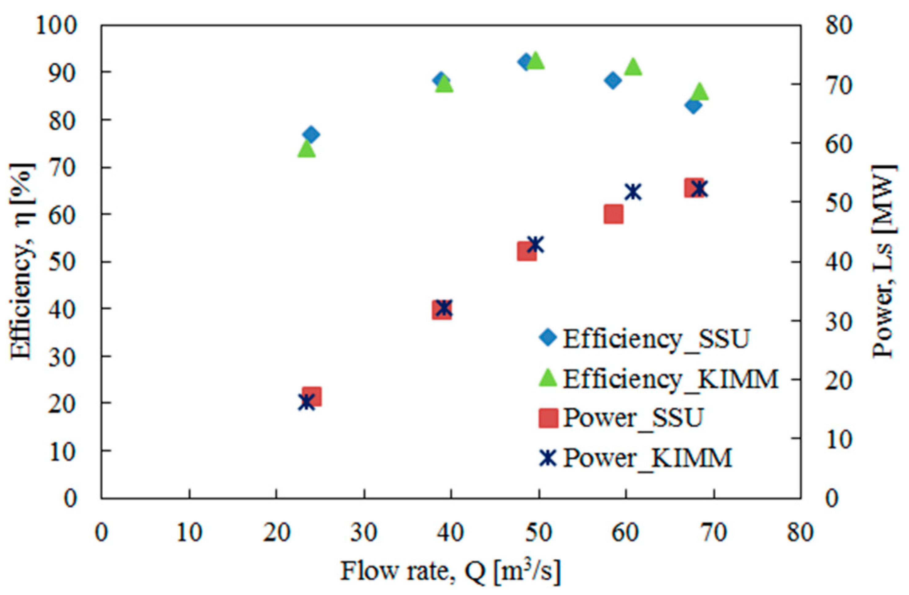
Numerical simulations were investigated at different flow rates by varying the guide vane opening angles of the prototype turbine. The guide vane opening angles were set to 10°, 16°, 20°, 25°, and 30°. Figure 5 illustrates the performance characteristics of the simulation results for the prototype turbine of Soongsil University (SSU) and Korea Institute of Machinery and Materials (KIMM). From the data for the SSU, it can be seen that the maximum efficiency found was 92.398%, and output power was 41.957 MW at a flow rate of 48.596 m3/s.
The preliminary experiment was conducted at Fuji Electric Co., Ltd. test facility. Moreover, the scale model experimental tests were conducted at KIMM, Korea. The experimental measurements, and calibrations were carried out using the procedure and guidelines IEC-60193 [50]. The flow similarity (1:10) was performed according to IEC-60193. In particular, IEC-60193 applies to any type of reaction turbine or impulse turbine tested under specified laboratory circumstances and may accordingly be utilized for acceptance tests of the prototype turbines as well [50]. The test facility was designed and established at the KIMM and designed to meet IEC 60193 [50]. Figure 6 shows the KIMM test facility measurement system. In the KIMM laboratory, the hydraulic Francis turbine performance test facility was carried out using a closed-loop circulation method using pressure drop measurement and flow rate measurement devices. The four pressure sensors were installed located at the turbine inlet and draft tube outlet to measure the differential pressure (Figure 6). Flow rate was measured by the electromagnetic flow meter. Data from the equipment were accounted for using a control computer. A total of 16 different pressure values were measured during the test. Uncertainties in a hydraulic turbine were estimated [50,51,52] and included random, systematic, and spurious errors. The systematic uncertainty in hydraulic turbine efficiency was calculated from the individual uncertainties in discharge (fQ)sys, specific hydraulic energy (fE)sys, torque (fT)sys, rotational speed (fn)sys, and density of water (fρ)sys:
At a 95% confidence level and 15 df, the random uncertainty in hydraulic turbine efficiency was estimated. The normal distribution of the efficiency was η ±0.221%, and the total hydraulic efficiency (fnh)total was calculated and found to lie within a band of ±1.224%. The measurement was carried out only one operating point (GV-20°). Therefore, only one measurement data could not illustrate the 95% confidence limit and error propagation from the result (Table 4).
Further, the numerical simulation results were validated with experimental data. Table 4 illustrates the CFD performances and the experimental results for the prototype turbine at design operating condition (GV-20°) [53]. As shown in the Table 4, prototype simulation was also done at SSU laboratory and at KIMM, and a reverse design was also done at KIMM. The maximum difference in efficiency was only 0.958% compared with the SSU simulation, 1.0485% compared with the KIMM (reverse design), 0.6088% compared with the KIMM simulation, and 0.547% compared with the experiment (KIMM). However, for the comparison of SSU results, it was 0.08% with KIMM (reverse design), 0.351% with KIMM modeled, and 0.413% with KIMM experiment values. It was also observed that SSU CFD results tended to have a slightly lower pre-experiment and experiment value but a steadily higher value of reverse design. With both results similar, there was good agreement between the results, indicating reliability.
4.2. Erosion Effects on Performance Characteristics
4.2.1. Effect of Sediment Inflow Rates
To look into the effect of flow rates on erosion, different sediment inflow rates were taken into account and were ranging from 1 to 100 kg/s in the prototype turbines. Three guide vane opening angles (GV-16°, GV-20°, GV-25°) were chosen for computer simulations namely the part load (GV-16°), best efficiency (GV-20°), and full load condition (GV-25°), while other working conditions remained constant. Only sediment inflow rates were selected while other parameters such as shape, sediment size, and impingement angle were kept constant in the Tabakoff–Grant erosion model. The effects of predicted sediment inflow rates on the turbine blade are illustrated in Figure 7, both in terms of best efficiency and full load operating conditions at the pressure side. It can be seen from these figures that as the flow rates grew, the area of the erosion rate density also become grown. At full load condition, the erosion rate density was higher than that of the best efficiency because the flow rate increase brought in a higher relative velocity at the outlet area of the runner vane. To better comprehend the visualized erosion of the runner blade of the prototype turbine, Figure 7a illustrates the best efficiency conditions. Estimated erosion regions can be separated into three segments, namely the leading edge side (Figure 7(1)), the trailing edge side (Figure 7(2)), and the outlet side (Figure 7(3)). It can also be observed from these graphs that the area of severe erosion rate density happened at the trailing edge of the runner vane. At the leading edge side, the erosion rate density was low, and only a small region was affected by the area of erosion rate. This occurred as the highest acceleration region was found throughout the inlet and the leading edge side of the runner vane. At the trailing edge, the erosion area grew because of the high relative velocity, and at this section, the area of severe erosion rate density was greatest. In the circumstances, the erosion area was higher than both of the outlet side and the leading edge side owing to the fact that the velocity was highest at the outlet region of the runner.
Moreover, on account of high relative velocity, the majority of the sand particles carried toward the outer diameter in the runner blade outlet, and, therefore, greater influence of erosion patterns can be observed there. This can be established by the velocity distribution inside the runner as shown in Figure 8a. These simulations revealed that a strong erosion pattern can be observed in the trailing edge of the runner blade from which the water exits and the outlet area that contacts the outlet part. Particularly, the outlet region shows strong erosion intensity, and the extent of erosion is widely spread out. As can be seen in Figure 8b, it is considered that the erosion rate is proportional to the power of the velocity. It is also observed that velocity is significantly increased at the outlet region where the relative velocity of the water moving out to the draft tube is the greatest (marked dotted circle). The predicted erosion rate density on the suction side of the blade is less than on the pressure side. This is even more in a wider guide vane opening. The erosion rate density is higher toward the outlet as compared to the inlet of the blade.
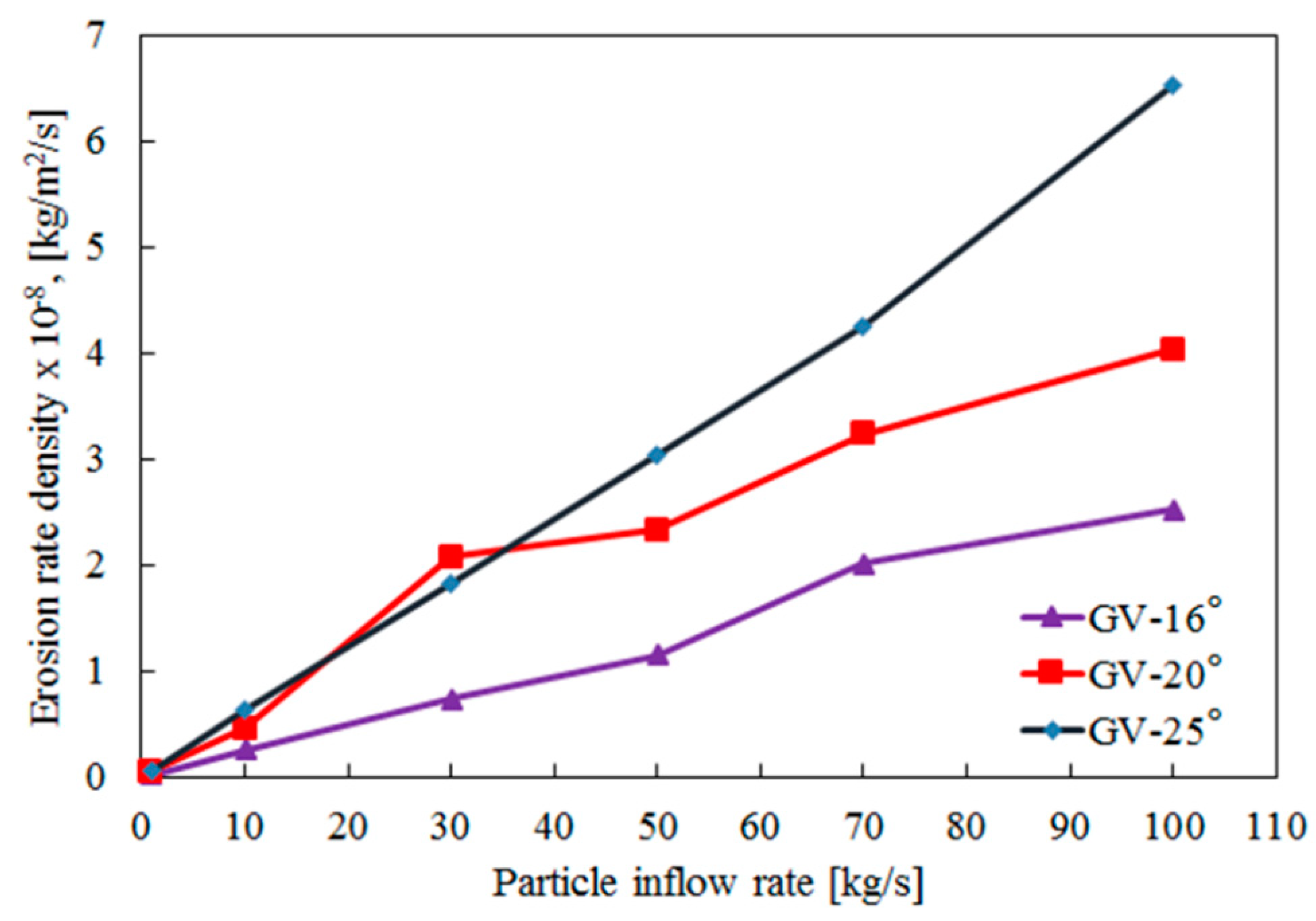
In addition, in the turbine model, the variations of the averaged erosion rate density of the runner blades with different sediment inflow rates (1–100 kg/s) are illustrated in Figure 9 at three different operating conditions. Three guide vane opening angles (GV-16°, GV-20°, and GV-25°) were selected for comparison. It can be observed from the graph that the erosion rate density increases in a nearly linear correlation at the three different operating conditions. The erosion rate was almost steady according to a given particle flow rates and guide vane opening. It can also be seen that a higher erosion rate occurred at a 25° opening angle than for the part load and the rated operating conditions.
4.2.2. Influence of Sediment Particle Shape Factor
In this current work, the various shape factors of the particles, i.e., 1, 0.75, 0.5, and 0.25, were investigated. Simulations were performed at given particle inflow rates for best efficiency condition while other operating conditions were kept constant. Particle shape factor is equal to one that implies that the shape of the particle is nearly the same with the spherical shape. When the shape of the particle is less or more than the regular shape, then particle behavior is changed to the irregular shape of the particle, i.e., nonspherical particle. In other words, the lower value of the shape factor causes a more asymmetrical shape on the particles. The effect of erosion rate density on turbine blade due to the shape factor is presented in Figure 10 that depicts the prediction of erosion rate density along the blade surface at 20° guide vane opening, which is at the best efficiency. It is revealed from the figure that at guide vane angle of 20°, higher erosion patterns take place in the blade profile with shape factor 0.5. This can be affected both by mass and heat transfer relation and, hence, erosion divination. Moreover, it is clearly observed in the case of the nonspherical shape of the particle that the blade region is greatly affected, and that larger intensity of the erosion rate has occurred at the trailing edge of the runner blade. It is seen from the figure that at full load condition (at guide vane angle of 25°), the turbine blade region is mostly influenced by the particle erosion rate at the trailing edge side. It is also shown that from simulations, the predicted erosion rate density is higher at full load condition than that of the rated condition. This occurs owing to the increased flow rate, the existence of secondary flows, and the generated vortices that lead to increased local velocities, higher relative motion, and potential separation of flow inside the turbine.
4.3. Cavitation-Erosion Effects
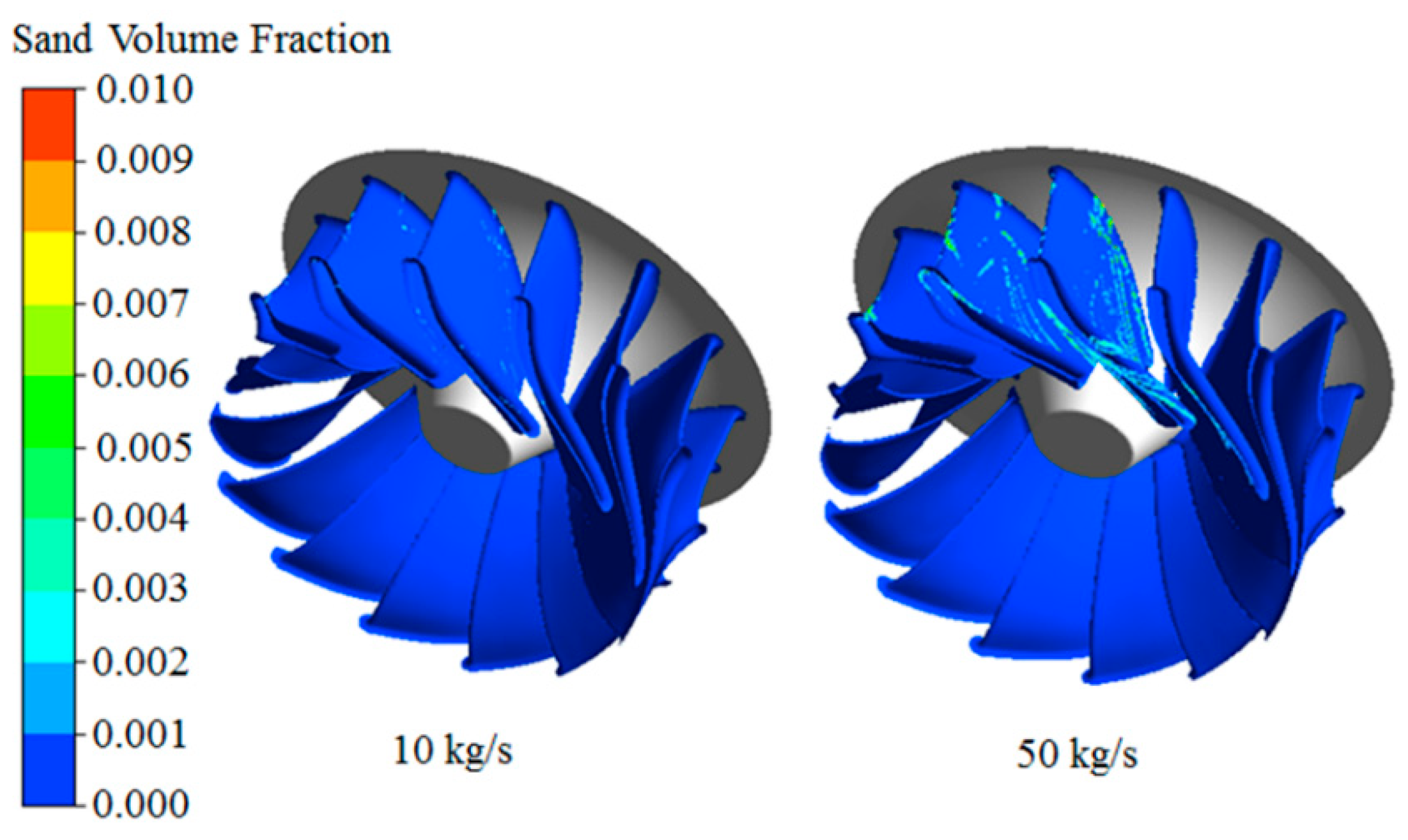
Generally, in the cavitating condition, water carries bubbles into the high regions of higher pressure, but in the case of cavitation–erosion, water, as well as sediment, carries the vapor bubbles into the high-pressure region [21]. For that reason, cavitation–erosion is more important than the normal cavitation condition. In this study, cavitation performance was investigated under integrated cavitation–sand erosion at three different sand inflow rates (10 kg/s, 50 kg/s, and 70 kg/s). Simulations were performed at the best efficiency (GV-20°) and full load condition (GV-25°), while other conditions kept constant. Figure 11 presents the combined cavitation erosion water vapor distributions on the runner blade. It is obvious to see from this figure that as the particle flow rates increased, the area of the attached cavitation also increased from the trailing edge at the suction side. The distributions of the sand volume fraction are depicted in Figure 12, in which the distributions of the sand vapor fraction increased with increasing sediment inflow rates in the turbine. Cavitation abrasion propagation mainly emerged at the leading edge pressure side to the trailing edge of the runner, and this study noticed that the sand volume distribution was nonuniform. A small sand cavity happened at the suction side of the runner blade, and the distributed blade pressure side revealed nonuniformity, which was a result of the combined vapor–sand effect, reducing efficiency.
4.4. Comparison of Performances at Different Sand Inflow Rates
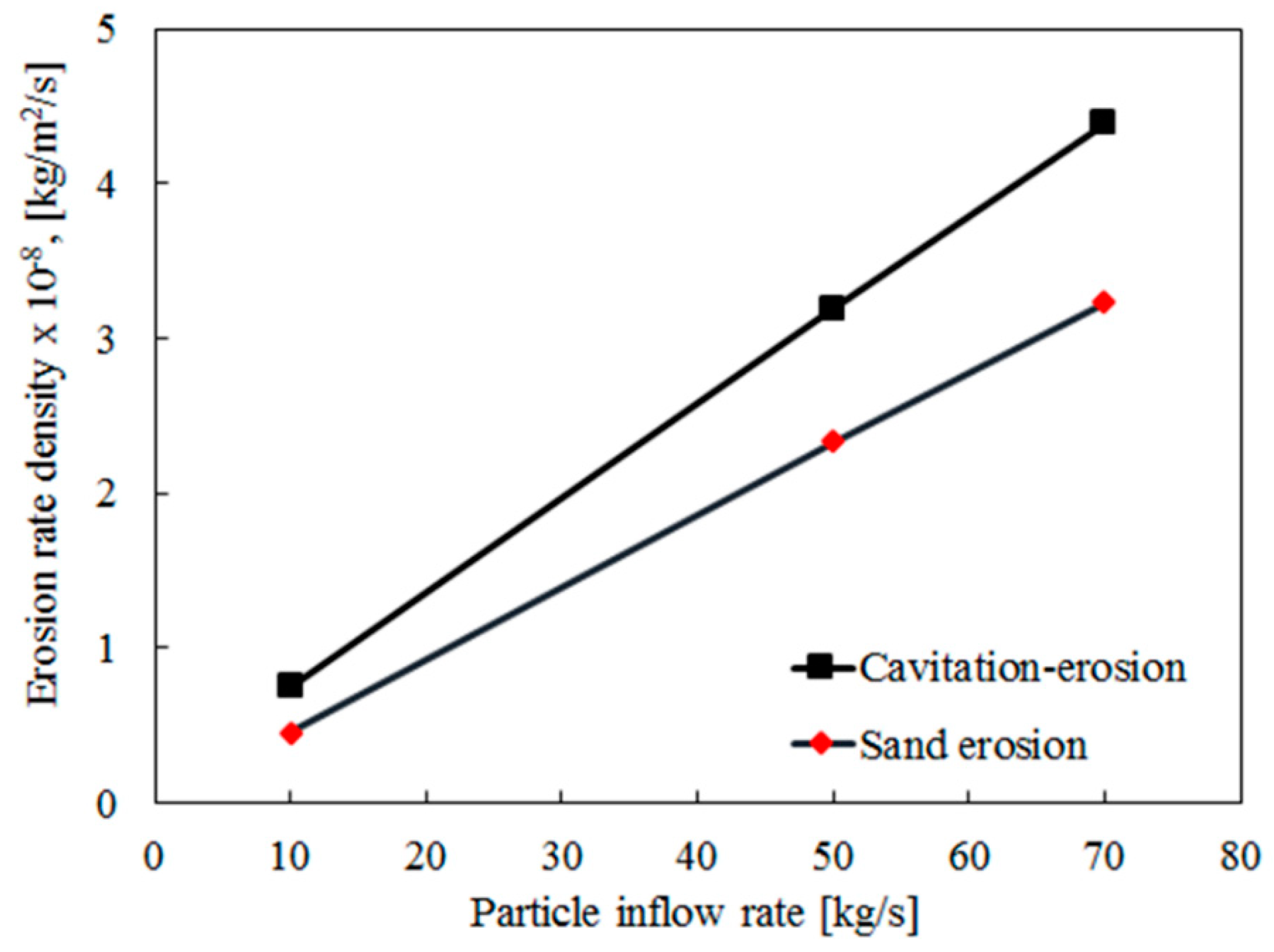
In this work, the efficiency of the Francis turbine was estimated for different sediment flow rates at best efficiency (GV-20°) operating condition. Numerical simulation results can be seen in Figure 13, which depicts sand erosion and cavitation–sand erosion conditions and shows a comparison of the computed efficiencies under sand erosion and cavitation–sand erosion at different sand inflow rates. It is obvious from the figure that efficiency is sharply decreased with increases in sand inflow rates. One notices that cavitation–sand erosion operation efficiency was reduced to a greater extent than the sand erosion condition. On top of this, the maximum efficiency dropped by 0.85% compared to sand erosion at the inflow rates of 70 kg/s, and maximum efficiency reduced by 1.33% compared to the pure water (single-phase) flow as shown in Figure 14. Additionally, a contrast of erosion rate density of sand erosion and cavitation–sand erosion is shown in Figure 15, where results show that, under cavitation–sand erosion condition, the erosion rate is higher compared to the sand erosion condition.
5. Conclusions
The main topic of this study was to look into the flow of sediment erosion on a Francis turbine with different operating conditions. In all cases, a perfect initial turbine without any changes of the geometry was investigated. In a real-world case, erosion and cavitation may trigger an increase impact; in the prototype model, the computed performance was compared with experimental data at optimal efficiency conditions and a good agreement occurred between them. To investigate sediment erosion on the turbine, the Tabakoff–Grant erosion model was adapted to simulate sand erosion characteristics. The current research notices that the maximum possible erosion areas were mostly found on the pressure side of the runner blades. The eroded region throughout the leading edge side is considered to be due to high acceleration. The area around the trailing edge and outlet side is arisen from the higher velocity around the outlet side of the runner. Additional simulations were then performed to analyze the effect of sediment inflow rates and sediment shape factors. This work found that as the sediment inflow rates increased in the prototype turbine, the erosion rate density increased in a near-linear fashion. Therefore, when the sediment flow rate is given, it is likely that potential erosion damage can be estimated by utilizing this linear correlation. The influences of erosion rate density on the turbine blade owing to shape factor and sediment size was also mentioned by this research. In addition to, in cavitation–sand erosion, this study notices that the low-sand volume fraction happened at the inlet near the suction side and the higher volume fraction of sand was visible at the trailing edge and outlet of the runner blade at the pressure side. From this work’s analysis, it was also suggested that cavitation abrasion propagation began mostly from the leading-edge pressure side to the trailing edge of the runner and that the sand volume fraction was disseminated nonuniformly. As the sediment flow rate increased within the area of the attached cavitation so too did it increase from the trailing-edge at suction side. Cavitation–erosion results also noticed that the efficiency reduced by 0.85% compared to sand erosion, and 1.33% compared to pure water. The numerical model itself is validated with the experimental data, but the novelty is in this erosion model. Instead, such a comparison should be conducted for verification of the investigated model. Consequently, if the curvature at the trailing edge and, in particular, at the outlet side of the runner is considered special consideration during the design, development, and optimization stages, it is possible to reduce cavitation and sediment erosion.
Author Contributions
M.R. conceived, designed, analyzed the results and wrote the paper; H.-H.K. managed project administration and edited the draft; K.K. contributed in result analysis; S.-H.S. contributed in fund collection, reviewed the work totally; K.Y.K. advised the project work.
Funding
This research was funded by Korea Technology and Information Promotion Agency for SMEs grant number S8025391.
Acknowledgments
This research was supported by the Korea Technology and Information Promotion Agency for SMEs (TIPA). The grant number is S8025391.
Conflicts of Interest
The authors declare no conflict of interest.
Nomenclature
| CFD | Computational Fluid dynamics |
| GCI | Grid convergence index |
| KIMM | Korea Institute of Machinery and Materials |
| SSU | Soongsil University |
| C | Concentration of particle, kg/m3 |
| c | Velocity of particle, m/s |
| df | Degree of freedom |
| E | Erosion rate, mm/yr |
| f(α) | Function of impingement angle |
| f(Vpn) | Function of velocity of particle |
| f | Uncertainty |
| Kmat | Material constant |
| Kenv | Environmental constant |
| k1, k2, k3, k4, k12 | Variable constant |
| Mass of the particle | |
| Mr | Coefficient of water resistance |
| Number rate | |
| n | Exponent number |
| Pf | Abrasive power |
| r | Grid ratio |
| Rθ | Tangential restitution factor |
| R | Radius of curvature on surface |
| S1 | Coefficient of sediment concentration |
| S2 | Coefficient of sediment hardness |
| S3 | Coefficient of sediment particle size |
| S4 | Coefficient of sediment shape |
| V | Velocity, m/s |
| Volume of particle | |
| Vp | Particle impact velocity, m/s |
| W | Erosion rate, mm/year |
| Greek Symbols | |
| α | Impingement angle, degree |
| β | Impact angle, rad |
| μ | coefficient of friction between particle and surface |
| ρ | Density, kg/m3 |
References
- Li, W.F.; Feng, J.J.; Wu, H.; Lu, J.L.; Liao, W.L.; Luo, X.Q. Numerical Investigation of Pressure Fluctuation Reducing in Draft Tube of Francis Turbines. Int. J. Fluid Mach. Syst. 2015, 8, 202–208. [Google Scholar] [CrossRef]
- Mann, B.S.; Arya, V. Abrasive and erosive wear characteristics of plasma nitriding and HVOF coatings: Their application in hydro turbines. Wear 2001, 249, 354–360. [Google Scholar] [CrossRef]
- Padhy, M.K.; Saini, R.P. A review on silt erosion in hydro turbines. Renew. Sustain. Energy Rev. 2008, 12, 1974–1987. [Google Scholar] [CrossRef]
- Sage, W.; Tilly, G.P. The significance of particles sizes in sand erosion of small gas turbines. R. Aeronaut. Soc. J. 1969, 73, 427–428. [Google Scholar] [CrossRef]
- Hussein, M.F.; Tabakoff, W. Dynamic Behavior of Solid Particles Suspended by Polluted Flow in a Turbine Stage. J. Aircr. 1973, 10, 434–440. [Google Scholar] [CrossRef]
- Hussein, M.F.; Tabakoff, W. Computation and plotting of solid particle flow in rotating cascades. Comput. Fluids 1974, 2, 1–15. [Google Scholar] [CrossRef]
- Grant, T.; Tabakoff, W. Erosion prediction in turbomachinery resulting from environmental solid particles. J. Aircr. 1975, 12, 471–547. [Google Scholar] [CrossRef]
- Hamed, A.; Tabakoff, W. Experimental and Numerical Simulations of the Effects of Ingested Particles in Gas Turbine Engines. In AGARD Conference Proceedings; AGARD: London, UK, 1994; p. 11. [Google Scholar]
- Ghenaiet, A. Modeling of Particle Trajectory and Erosion of Large Rotor Blades. Int. J. Aerosp. Eng. 2016, 2016, 7928347. [Google Scholar] [CrossRef]
- Thapa, B.S.; Dahlhaug, O.G.; Thapa, B. Sediment erosion in hydro turbines and its effect on the flow around guide vanes of Francis turbine. Renew. Sustain. Energy Rev. 2015, 49, 1100–1113. [Google Scholar] [CrossRef]
- Tang, J.; Chai, L.; Li, H.; Yang, Z.; Yang, W. A 10-Year Statistical Analysis of Heavy Metals in River and Sediment in Hengyang Segment, Xiangjiang River Basin, China. Sustainability 2018, 10, 1057. [Google Scholar] [CrossRef]
- Zhang, J.; Hu, Q.; Wang, S.; Ai, M. Variation Trend Analysis of Runoff and Sediment Time Series Based on the R/S Analysis of Simulated Loess Tilled Slopes in the Loess Plateau, China. Sustainability 2018, 10, 32. [Google Scholar] [CrossRef]
- Alam, S. Essential design features for efficient sediment management. Int. J. Hydropower Dams 2005, 12, 80–83. [Google Scholar]
- Chamoun, S.; De Cesare, G.; Schleiss, A.J. Managing reservoir sedimentation by venting turbidity currents: A review. Int. J. Sediment Res. 2016, 31, 195–204. [Google Scholar] [CrossRef]
- Schleiss, A.J.; Franca, M.J.; Juez De Cesare, G. Reservoir sedimentation. J. Hydraul. Res. 2016, 54, 595–614. [Google Scholar] [CrossRef]
- Pandit, H.P.; Shakya, N.M.; Stole, H.; Garg, N.K. Sediment exclusion in Himalayan rivers using hydro cyclone. J. Hydraul. Eng. 2008, 14, 118–133. [Google Scholar]
- Gabl, R.; Gems, B.; Birkner, F.; Hofer, B.; Aufleger, M. Adaptation of an Existing Intake Structure Caused by Increased Sediment Level. Water 2018, 10, 1066. [Google Scholar] [CrossRef]
- Thapa, B.; Upadhyay, P.; Dahlhaug, O.G.; Timsina, M.; Basnet, R. HVOF coatings for erosion resistance of hydraulic turbines: Experience of Kaligandaki-A Hydropower Plant. In Proceedings of the 2 International Symposium on Water Resources and Renewable Energy Development in Asia, Danang, Vietnam, 10–11 March 2008. [Google Scholar]
- Egusquiza, E.; Valero, C.; Estévez, A.; Guardo, A.; Coussirat, M. Failures due to ingested bodies in hydraulic turbines. Eng. Fail. Anal. 2011, 18, 464–473. [Google Scholar] [CrossRef]
- Weili, L.; Jinling, L.; Xingqi, L.; Yuan, L. Research on the cavitation characteristic of Kaplan turbine under sediment flow condition. IOP Conf. Ser. Earth Environ. Sci. 2010, 12, 012022. [Google Scholar] [CrossRef]
- Hua, H.; Zeng, Y.-Z.; Wang, H.-Y.; Ou, S.-B.; Zhang, Z.-Z.; Liu, X.-B. Numerical analysis of solid–liquid two-phase turbulent flow in Francis turbine runner with splitter blades in sandy water. Adv. Mech. Eng. 2015, 1–10. [Google Scholar] [CrossRef]
- Rakibuzzaman, M.; Kim, K.; Suh, S.H. Numerical and experimental investigation of cavitation flows in a multistage centrifugal pump. J. Mech. Sci. Tech. 2018, 32, 1071–1078. [Google Scholar] [CrossRef]
- Kumar, D.; Bhingole, P.P. CFD based analysis of combined effect of cavitation and silt erosion on Kaplan turbine. Mater. Today Proc. 2015, 2, 2314–2322. [Google Scholar] [CrossRef]
- Rakibuzzaman, M.; Kim, H.-H.; Park, N.; Suh, S.-H. Numerical Prediction of Sediment Erosion due to Sediment Concentrations in Francis Turbine. In Proceedings of the 7th Asia-Pacific Forum on Renewable Energy (AFORE), Busan, Korea, 15–18 November 2017. [Google Scholar]
- Thapa, B.S.; Thapa, B.; Eltvik, M.; Gjosater, K.; Dahlhaug, O.G. Optimizing runner blade profile of Francis turbine to minimize sediment erosion. In Proceedings of the 26th IAHR Symposium on Hydraulic Machinery and systems, Beijing, China, 19–23 August 2012. [Google Scholar]
- Duan, C.G.; Karelin, V.Y. Abrasive Erosion and Corrosion of Hydraulic Machinery; Imperial College Press: London, UK, 2002. [Google Scholar]
- Truscott, G.F. A literature survey on abrasive wear in hydraulic machinery. Wear 1972, 20, 29–50. [Google Scholar] [CrossRef]
- Neopane, H.P. Sediment Erosion in Hydro Turbines. Ph.D. Thesis, Norwegian University of Science and Technology, Trondheim, Norway, 2010. [Google Scholar]
- Pereira, G.C.; Souza, F.J.; Martins, D.A. Numerical prediction of the erosion due to particles in elbows. Powder Technol. 2014, 261, 105–117. [Google Scholar] [CrossRef]
- Bergeron, P. Consideration of the factors influencing wear due to hydraulic transport of solid materials. In Proceedings of the 2nd Conference on Hydraulic Transport and Separation of Solid Materials, Société Hydrotechnique de France, Paris, France, June 1952. [Google Scholar]
- Bergeron, P.; Dollfus, J. The influence of nature of the pumped mixture and hydraulic characteristics on design and installation of liquid/solid mixture pumps. In Proceedings of the 5th Conference on Hydraulics, January 1958; Volume 2, pp. 597–605. [Google Scholar]
- Bovet, T. Contribution to study of the phenomenon of abrasive erosion in the realm of hydraulic turbines. Bull. Tech. Suisse Romande 1958, 84, 37–49. [Google Scholar]
- Finnie, I. Erosion of Surfaces by Solid Particles. Wear 1960, 3, 87–103. [Google Scholar] [CrossRef]
- Hutchings, I.M. Tribology, Friction and Wear of Engineering Materials, 1st ed.; Elsevier Limited: Oxford, UK, 1992. [Google Scholar]
- Ansys Inc. ANSYS-CFX (CFX Introduction, CFX Reference Guide, CFX Tutorials, CFX-Pre User’s Guide, CFX-Solver Manager User’s Guide, Theory Guide), Release 16.00; Ansys Inc.: Canonsburg, PA, USA, 2016. [Google Scholar]
- Kang, M.-W.; Park, N.; Suh, S.-H. Numerical study on sediment erosion of Francis turbine with different operating conditions and sediment inflow rates. Procedia Eng. 2016, 157, 457–464. [Google Scholar] [CrossRef]
- Trivedi, C.; Cervantes, M.J.; Gandhi, B.K.; Dahlhaug, O.G. Experimental and Numerical Studies for a High Head Francis Turbine at Several Operating Points. ASME J. Fluids Eng. 2013, 135, 111102–111117. [Google Scholar] [CrossRef]
- Bergstrom, J.; Gebart, R. Estimation of Numerical Accuracy for the Flow Field in a Draft Tube. Int. J. Num. Meth. Heat Fluid Flow 1999, 9, 472–486. [Google Scholar] [CrossRef]
- Celik, I.B.; Ghia, U.; Roache, P.J.; Freitas, C.J.; Coleman, H.; Raad, P.E. Procedure for Estimation and Reporting of Uncertainty due to Discretization in CFD Applications. ASME J. Fluids Eng. 2008, 130, 078001. [Google Scholar]
- Fernandez-Gamiz, U.; Errasti, I.; Gutierrez-Amo, R.; Boyano, A.; Barambones, O. Computational Modelling of Rectangular Sub-Boundary Layer Vortex Generators. Appl. Sci. 2018, 8, 138. [Google Scholar] [CrossRef]
- Roache, P.J. Conservatism of the Grid Convergence Index in Finite Volume Computations on Steady-State Fluid Flow and Heat Transfer. ASME J. Fluids Eng. 2003, 125, 731–735. [Google Scholar] [CrossRef]
- Cadafalch, J.; Perez-Segarra, R.; Consul, R.; Oliva, A. Verification of Finite Volume Computations on Steady State Fluid Flow and Heat Transfer. J. Fluids Eng. 2002, 124, 11–21. [Google Scholar] [CrossRef]
- Mortiz, R. Transient CFD-Analysis of a High Head Francis Turbine. Master’s Thesis, Norwegian University of Science and Technology, Trondheim, Norway, 2014. [Google Scholar]
- Friziger, J.H.; Peric, M. Computational Methods for Fluid Dynamics, 3rd ed.; Springer: New York, NY, USA, 2002. [Google Scholar]
- Choi, H.J.; Zullah, M.A.; Roh, H.W.; Ha, P.S.; Oh, S.Y.; Lee, Y.H. CFD validation of performance improvement of a 500 kW Francis turbine. Renew. Energy 2013, 54, 111–123. [Google Scholar] [CrossRef]
- Kim, H.-H.; Rakibuzzaman, M.; Kim, K.; Suh, S.-H. Flow and Fast Fourier Transform Analyses for Tip Clearance Effect in an Operating Kaplan Turbine. Energies 2019, 12, 264. [Google Scholar] [CrossRef]
- Wilcox, D.C. Turbulence Modeling for CFD, 1st ed.; DCW Industries, Inc.: La Cañada Flintridge, CA, USA, 1994. [Google Scholar]
- Menter, F.R. Two-Equation Eddy-Viscosity Turbulence Models for Engineering Applications. AIAA J. 1994, 32, 1598–1605. [Google Scholar] [CrossRef]
- Georgiadis, N.J.; Yoder, D.A.; Engblorn, W.B. Evaluation of modified two-equation turbulence models for jet flow predictions. AIAA J. 2006, 44, 3107–3114. [Google Scholar] [CrossRef]
- CEI/IEC-60193, Hydraulic Turbines, Storage Pumps and Pump-Turbines- Model Acceptance Tests; International Standard; International Electrotechnical Commission: Geneva, Switzerland, 1999.
- Longo, S.; Di Federico, V.; Chiapponi, L. Non-Newtonian power-law gravity currents propagating in confining boundaries. Environ. Fluid Mech. 2015, 15, 515–535. [Google Scholar] [CrossRef]
- Longo, S.; Di Federico, V.; Chiapponi, L. A dipole solution for power-law gravity currents in porous formations. J. Fluid Mech. 2015, 778, 534–551. [Google Scholar] [CrossRef]
- Rakibuzzaman, M.; Kim, H.-H.; Kim, K.; Park, N.; Suh, S.-H. Numerical study of sediment erosion and surface roughness analyses in Francis turbine. In Proceedings of the 11th International Conference on Computational Heat and Mass Transfer, Cracow, Poland, 21–24 May 2018. [Google Scholar]
Figure 1.
Prototype Francis turbine.

Figure 2.
3-D unstructured grids by parts of the Francis turbine (a) spiral casing, stay vane, and guide vane, (b) runner, and (c) draft tube.
Figure 2.
3-D unstructured grids by parts of the Francis turbine (a) spiral casing, stay vane, and guide vane, (b) runner, and (c) draft tube.
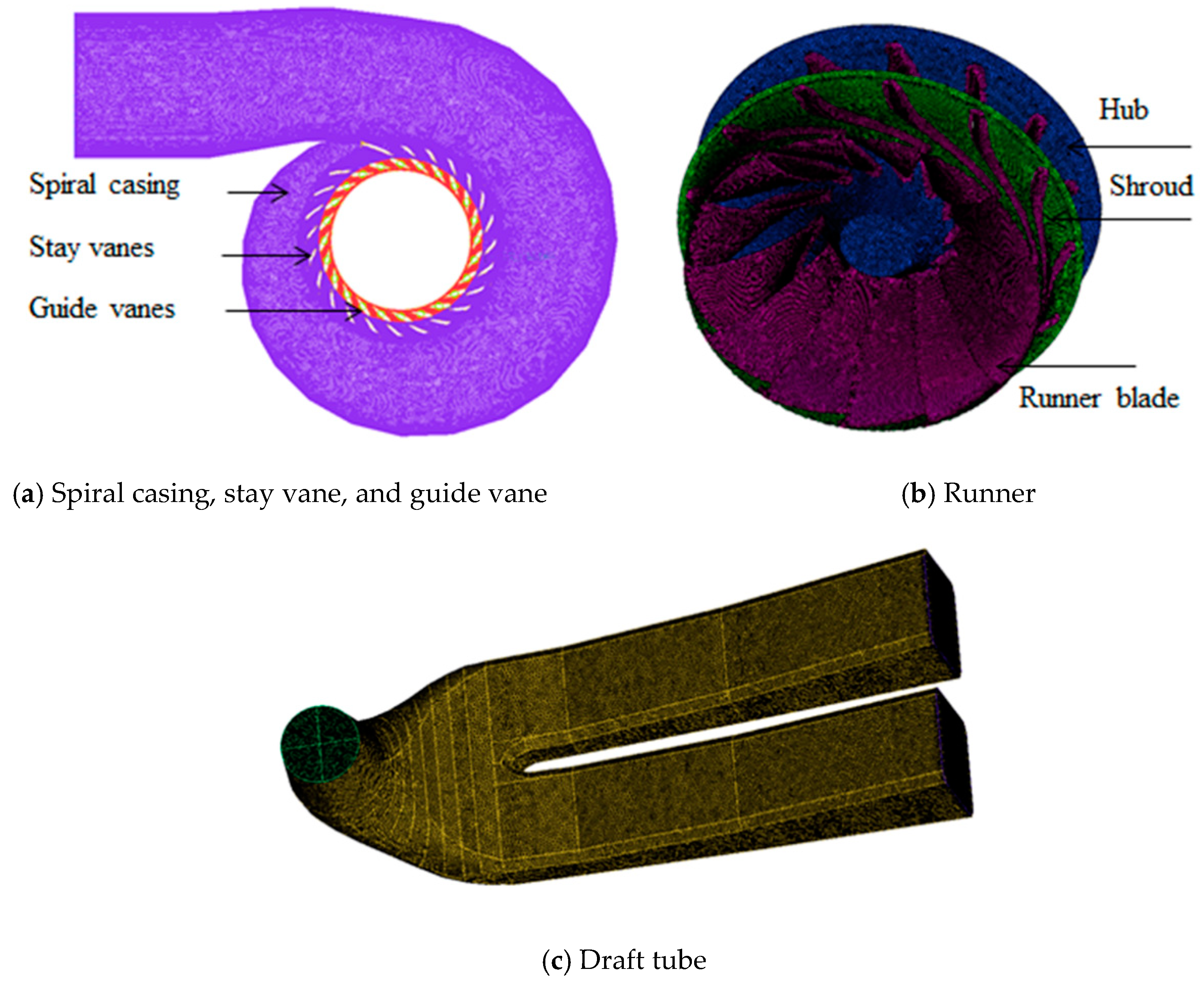
Figure 3.
Grid sensitivity test of the Francis turbine (vertical dotted line represents the used grid).
Figure 3.
Grid sensitivity test of the Francis turbine (vertical dotted line represents the used grid).
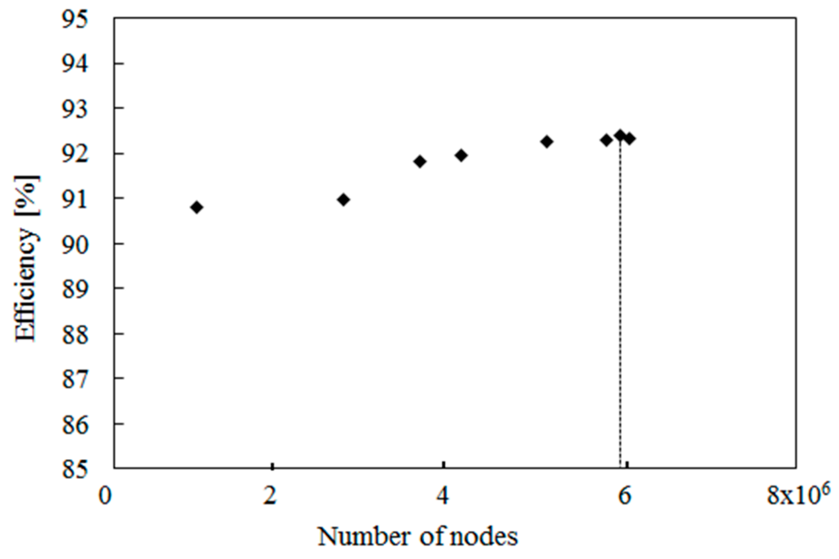
Figure 4.
Prototype turbine domain for computer simulation.
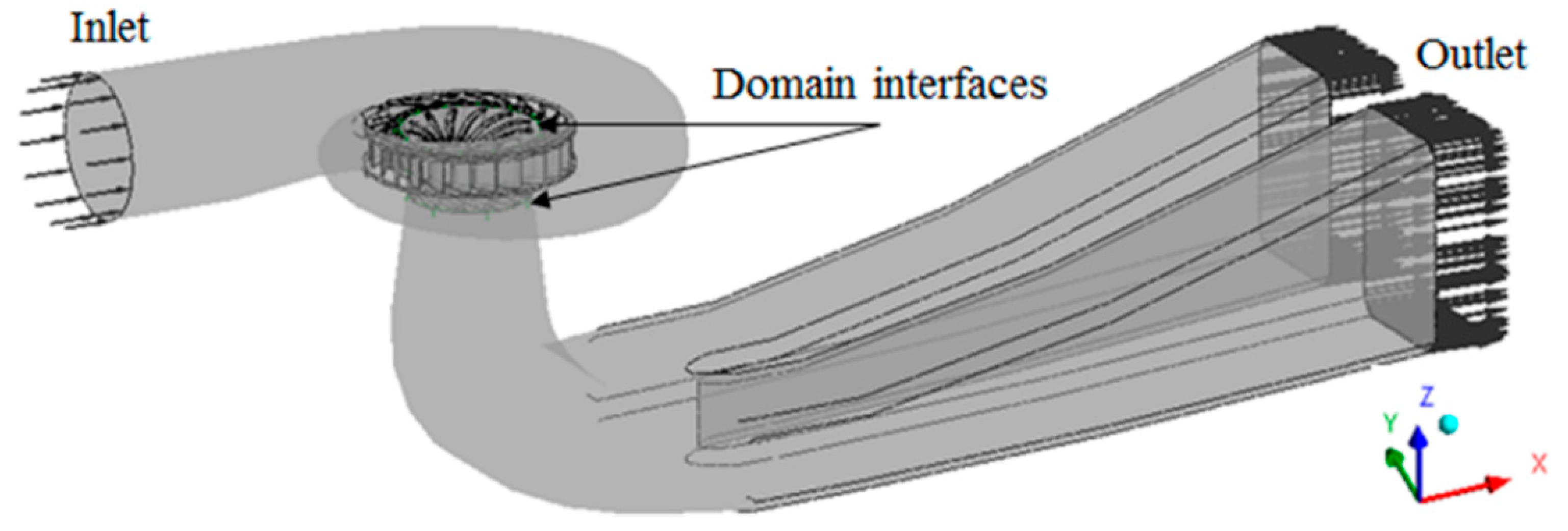
Figure 5.
Computed efficiencies and powers as a function of flow rates of the numerical simulation results for the prototype turbine. SSU: Soongsil University; KIMM: Korea Institute of Machinery and Materials.
Figure 5.
Computed efficiencies and powers as a function of flow rates of the numerical simulation results for the prototype turbine. SSU: Soongsil University; KIMM: Korea Institute of Machinery and Materials.

Figure 6.
Experimental facilities of a scale Francis turbine model of 1:10 at KIMM test site.

Figure 7.
Effect of sand flow rates on the sand rate density (a) best efficiency (GV-20°) and (b) full load (GV-25°) conditions.
Figure 7.
Effect of sand flow rates on the sand rate density (a) best efficiency (GV-20°) and (b) full load (GV-25°) conditions.
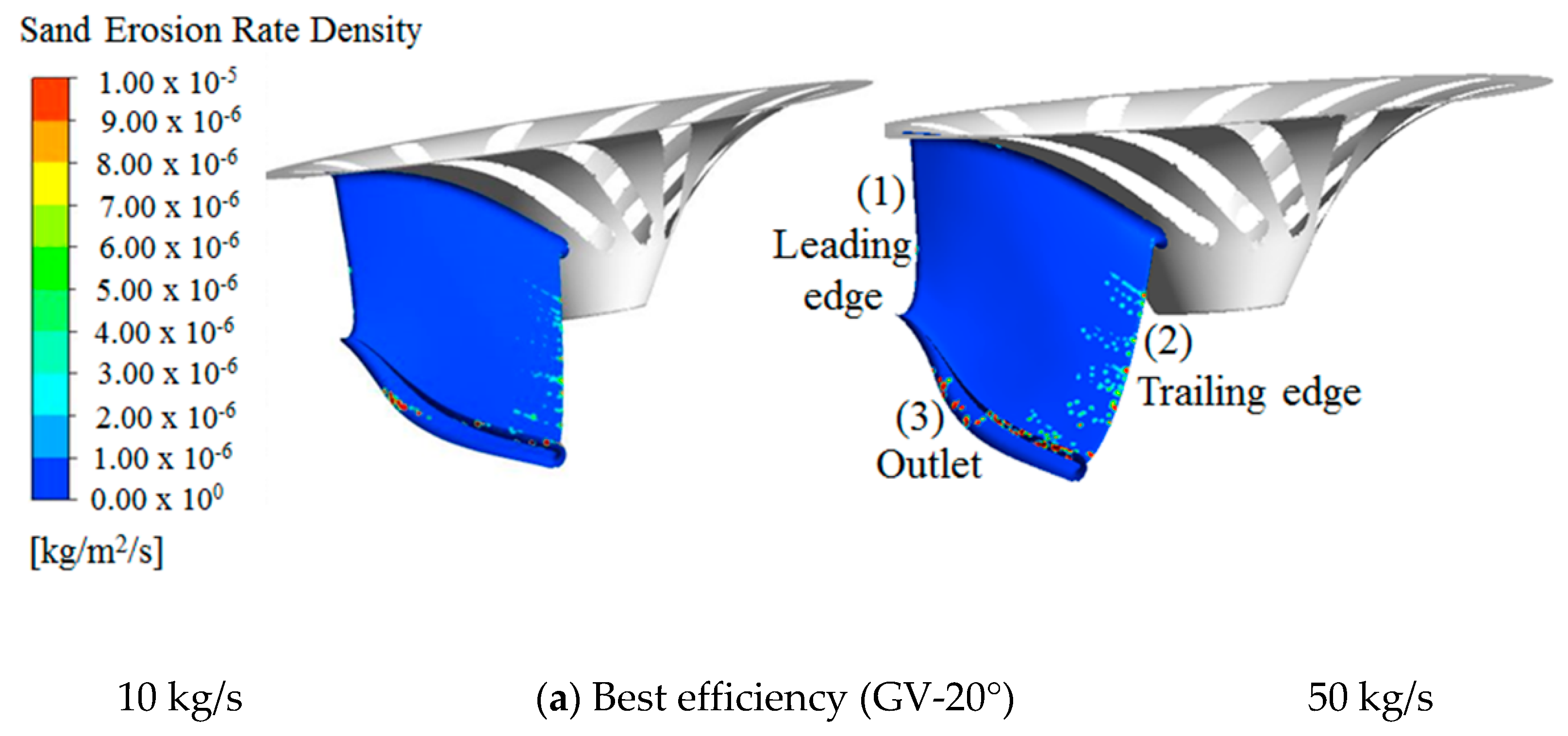

Figure 8.
Velocity distributions around the runner outlet on the (a) XY plane and (b) ZX plane.

Figure 9.
Erosion rate densities versus particle inflow rates at three guide vane opening angles (GV-16°, GV-20°, and GV-25°).
Figure 9.
Erosion rate densities versus particle inflow rates at three guide vane opening angles (GV-16°, GV-20°, and GV-25°).

Figure 10.
Sediment erosion rate density for different particle shape factors (0.5, 1.0) (a) best efficiency and (b) full load conditions.
Figure 10.
Sediment erosion rate density for different particle shape factors (0.5, 1.0) (a) best efficiency and (b) full load conditions.
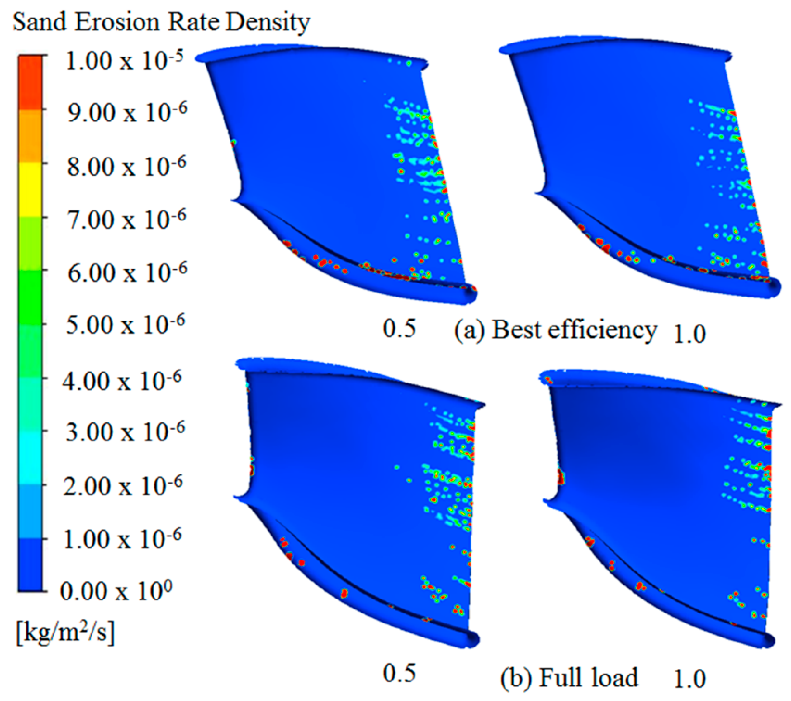
Figure 11.
Water vapor volume fraction contours on the runner at different sand inflow rates (10 kg/s, 50 kg/s).
Figure 11.
Water vapor volume fraction contours on the runner at different sand inflow rates (10 kg/s, 50 kg/s).
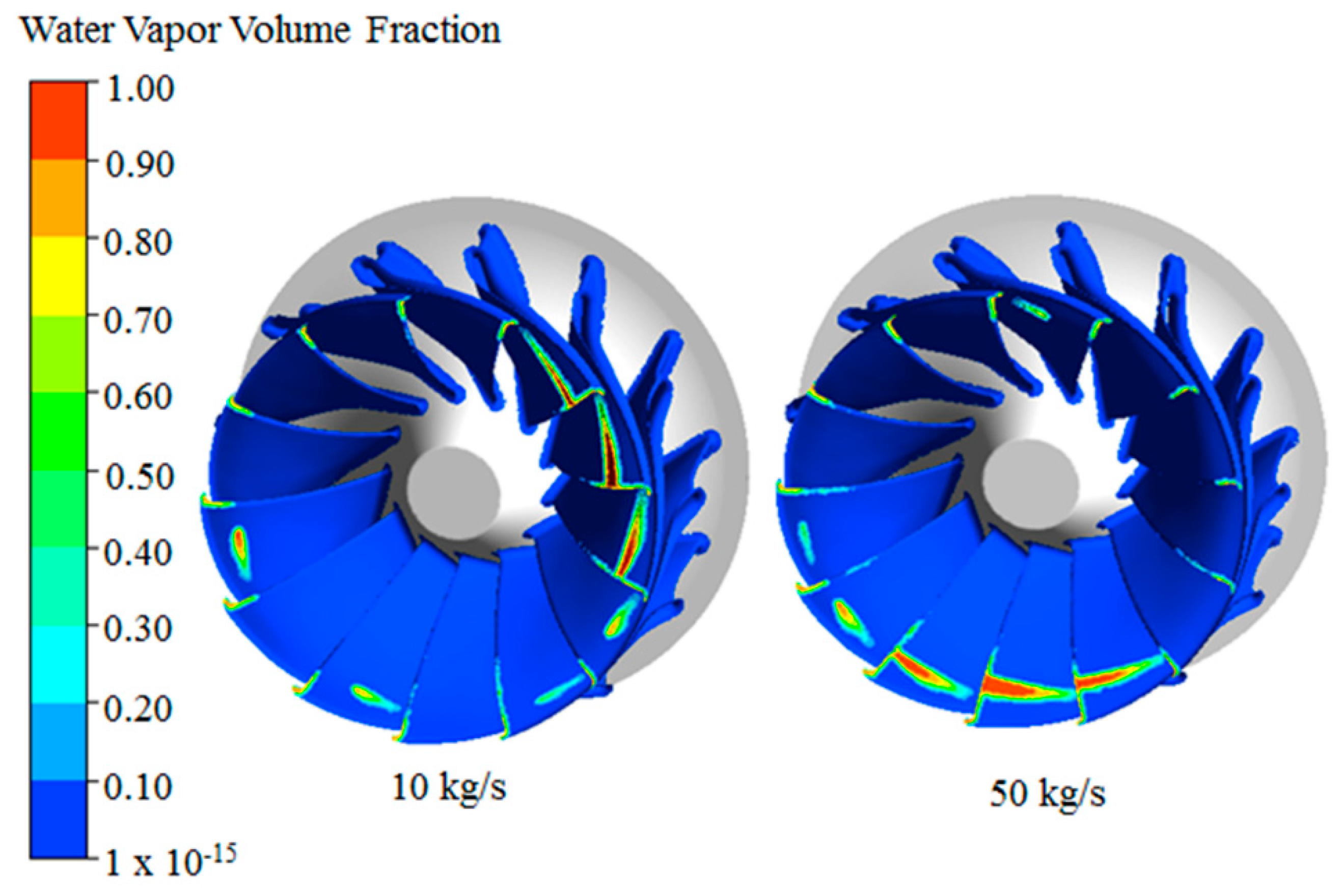
Figure 12.
Sand volume fraction contours on the runner at different sand inflow rates (10 kg/s, 50 kg/s).
Figure 12.
Sand volume fraction contours on the runner at different sand inflow rates (10 kg/s, 50 kg/s).

Figure 13.
The efficiency changes with different particle inflow rates at best efficiency (GV-20°).
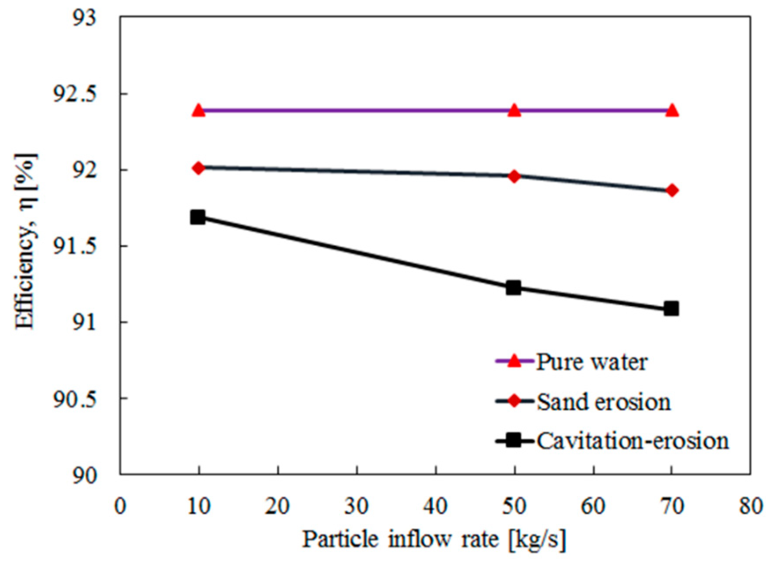
Figure 14.
Comparison of efficiency differences (water versus sand erosion, water versus cavitation-erosion, and sand erosion versus cavitation-erosion) with different particle inflow rates at best efficiency (GV-20°).
Figure 14.
Comparison of efficiency differences (water versus sand erosion, water versus cavitation-erosion, and sand erosion versus cavitation-erosion) with different particle inflow rates at best efficiency (GV-20°).
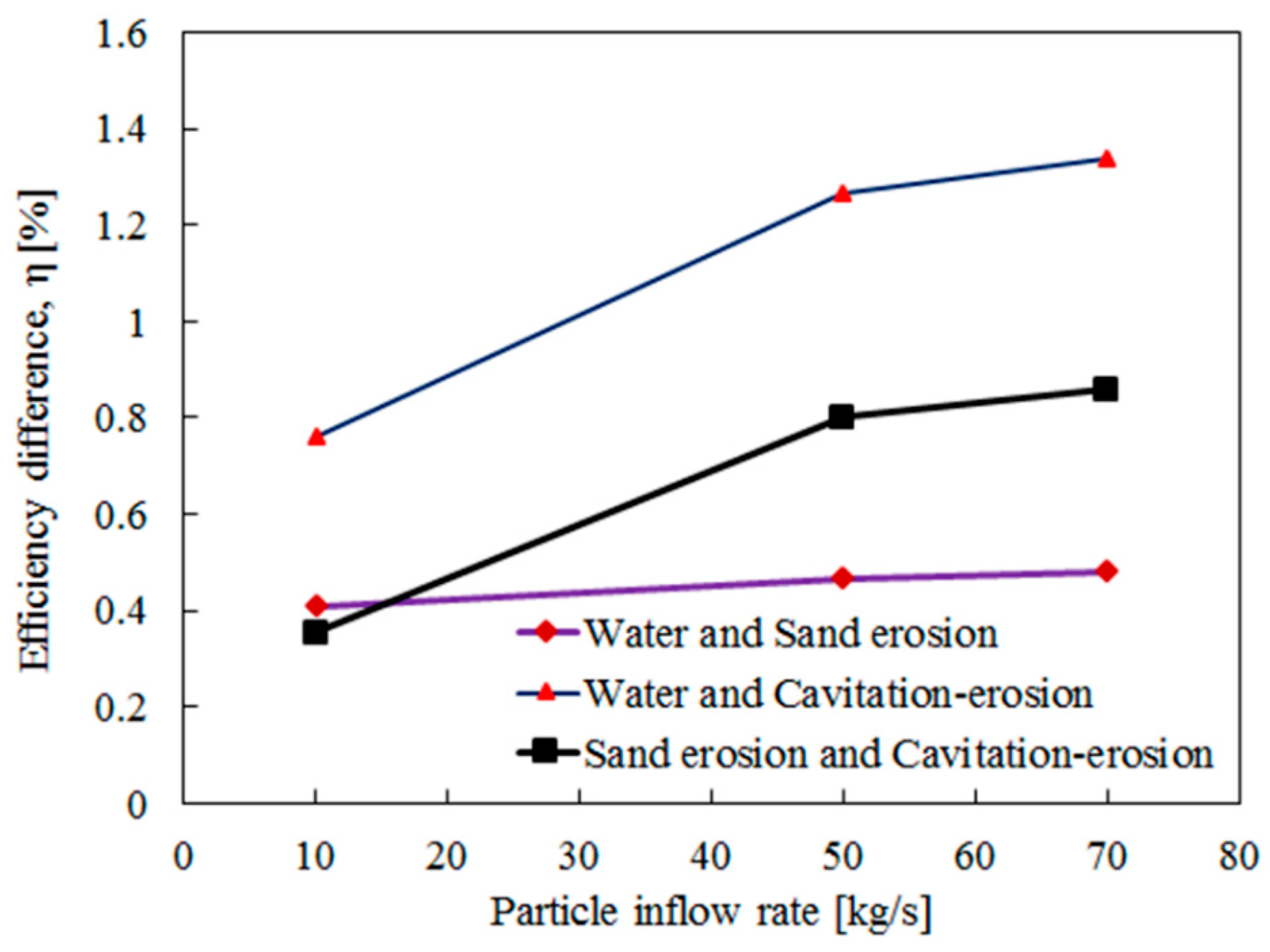
Figure 15.
Comparison of sand erosion and cavitation–erosion rate densities with different particle inflow rates at best efficiency (GV-20°).
Figure 15.
Comparison of sand erosion and cavitation–erosion rate densities with different particle inflow rates at best efficiency (GV-20°).


Table 1.
Specifications of the Francis turbine at Hapcheon hydropower plant, K-Water, Korea.
| Description | Dimension |
|---|---|
| Runner inlet diameter (mm) | 2728 |
| Runner outlet diameter (mm) | 2546 |
| Head (m) | 95 |
| Flow rate (m3/s) | 59.4 |
| Max. power (MW) | 51.6 |
| Rotational speed (rpm) | 257 |
| Runner blade | 13 |
| Guide vane | 24 |
| Stay vane | 23 |
Table 2.
Grid quality of the Francis turbine.
| Description | Elements | Nodes | Min. Y+ | Max. Y+ |
|---|---|---|---|---|
| Spiral casing | 14,552,267 | 246,6738 | 0.81 | 476 |
| Runner | 15,868,719 | 268,2908 | 2.71 | 274 |
| Draft tube | 4,368,719 | 785,142 | 1.58 | 66 |
| Total | 34,789,303 | 5,934,788 |
Table 3.
Grid convergence error and sensitivities in computational solutions.
| No. | Nodes | Grid Ratio, r | Efficiency (%) | Error, ea (%) | GCI |
|---|---|---|---|---|---|
| 1 | 963,652 | 2.788 | 90.82 | 0.1515 | 0.02844 |
| 2 | 2,686,965 | 1.337 | 90.96 | 0.9344 | 1.48009 |
| 3 | 3,594,116 | 1.133 | 91.81 | 0.1742 | 0.76761 |
| 4 | 4,072,292 | 1.245 | 91.97 | 0.3153 | 0.71562 |
| 5 | 5,071,234 | 1.170 | 92.26 | 0.1409 | 0.47659 |
| 6 | 5,934,788 | 1.020 | 92.39 | 0.0324 | 0.98898 |
| 7 | 6,055,348 | 0.102 | 92.36 | 0.0866 | 0.10943 |
Table 4.
Comparison of numerical simulations and experiment result for the turbine.
| Description | Efficiency (%) | Difference (%) |
|---|---|---|
| Pre-experiment (Fuji Electric Co.) | 93.292 (Exp.) | 0 |
| Reverse design (KIMM) | 92.324 (Sim.) | 1.0485 |
| Simulation (KIMM) | 92.724 (Sim.) | 0.6088 |
| Simulation (SSU) | 92.398 (Sim.) | 0.9579 |
| Experiment (KIMM) | 92.781 (Exp.) | 0.5477 |
© 2019 by the authors. Licensee MDPI, Basel, Switzerland. This article is an open access article distributed under the terms and conditions of the Creative Commons Attribution (CC BY) license (http://creativecommons.org/licenses/by/4.0/).
Share and Cite
MDPI and ACS Style
Rakibuzzaman, M.; Kim, H.-H.; Kim, K.; Suh, S.-H.; Kim, K.Y. Numerical Study of Sediment Erosion Analysis in Francis Turbine. Sustainability 2019, 11, 1423. https://doi.org/10.3390/su11051423
AMA Style
Rakibuzzaman M, Kim H-H, Kim K, Suh S-H, Kim KY. Numerical Study of Sediment Erosion Analysis in Francis Turbine. Sustainability. 2019; 11(5):1423. https://doi.org/10.3390/su11051423
Chicago/Turabian StyleRakibuzzaman, Md, Hyoung-Ho Kim, Kyungwuk Kim, Sang-Ho Suh, and Kyung Yup Kim. 2019. "Numerical Study of Sediment Erosion Analysis in Francis Turbine" Sustainability 11, no. 5: 1423. https://doi.org/10.3390/su11051423
Note that from the first issue of 2016, this journal uses article numbers instead of page numbers. See further details here.