Assessment of Wind Power Potential and Economic Analysis at Hyderabad in Pakistan: Powering to Local Communities Using Wind Power

Abstract

Wind power is the fastest growing and environmentally sustainable source of energy among all available renewable energy resources. The primary objective of this paper is to analyze the wind characteristics and power potential at Hyderabad, Southeastern province in Pakistan. Two years of wind speed data measured at 10 m above ground level (AGL) have been considered in this study. The annually, monthly, and seasonal variations in wind speed were analyzed, and minimum, maximum, and average values of recorded wind speeds are presented in this paper. Weibull and Rayleigh distribution functions have been applied to analyze the wind characteristics and evaluate the wind power potential of the proposed site. The Weibull shape k and scale c parameters have been estimated using the Weibull function. The higher values of k showed that the wind speed is steady at the site. The average wind speed was found above 6 m/s throughout the year. The most probable wind speed (V_mp) and maximum carrying energy (V_maxE) wind speed were also calculated using Weibull parameters. Root mean square error (RMSE), the coefficient of determination (R²), and mean bias error (MBE) were computed to ensure the good fit of Weibull distribution function. The annual average wind power and energy densities were estimated at more than 255 W/m² and 2245 kWh/m², respectively. The power density calculated by Weibull and Rayleigh functions was compared with that calculated by using measured wind data. The energy output and capacity factor of different commercially available wind turbines (WTs), i.e., power ratings from 0.33 to 2.75 MW, have been calculated. The cost of energy was estimated and ranged from $19.27 to $32.80 per MWh. Wind power potential and economic analysis of the collected data reveals that the site is suitable for developing wind power generation projects to power the local communities.

1. Introduction

The cost of the industrial revolution is a massive increase in the use of fossil fuels, which include coal, natural gas, oil, and gasoline, resulting in highly infected air. Due to this, global climate is changing and is affected severely; high amounts of greenhouse gases are emitted due to the mismanaged use of these fuels in a vast range of applications that can be found in producing and consuming energy. Carbon dioxide (CO₂) is one of the most common of these gases and is the leading cause of these changes in the behavior of the earth’s atmosphere. However, even this intensive use of resources cannot account for the high amounts of energy consumption of today’s age. Therefore, alternate resources need to be used to generate environmentally sustainable energy [1,2]. The most economically active energy resources are the solar, biomass, wind, and geothermal power. Among these resources, the wind power is the most affordable, efficient, and commonly used by many developed and developing countries and hence is considered as the first choice of energy resources [3,4]. Thirty-five percent of the world’s energy demand can be fulfilled if all the available wind power is consumed [5]. The installed wind energy capacity all over the globe increased to 539 GW by the end of 2017, which indicates the need and the worth of this energy source for the future [6]. The Global Wind Energy Council (GWEC), responsible for wind power industry trade throughout the world, is making efforts to make wind power a dominant resource for generating energy. According to the reports from the GWEC, China is the most dominant in making efforts to enforce changes and making a switch to new energy resources. Achieving 34% of the annual market, China installed 19.66 GW in 2017 and is currently the market leader with 188 GW power generated from the wind resources. The United States is in second place and Germany is in third with 89 GW and 56 GW, respectively [7]. With Pakistan’s negligible oil and gas reserves and high costs required for nuclear energy production, the use of alternate energy sources is essential to fulfilling the energy deficit of the country. The Pakistan Meteorological Department (PMD) conducts surveys to locate optimal locations for the wind and other alternative energy resources throughout the country. According to these reports, a potential corridor for good wind energy generation is about 1100 km, on the coastline of the Sindh and Baluchistan provinces [8].

In order to obtain the maximum efficiency and minimize investment risk of a wind project, it is imperative to assess the feasibility, operation cost, and energy potential before installing the wind energy system [9]. Many researchers have used several statistical descriptors and probability distributions to test and analyze the characteristics of wind data. For wind data and its analysis, Weibull and Rayleigh distributions provide the best fit of the data collected [10,11,12,13]. Weibull has become a standard due to its simplicity and flexibility, and, according to the international standard of the International Electrotechnical Commission (IEC: 614-00-12), two-parameter Weibull is a proper approach to analyze wind characteristics. These parameters—Weibull shape and scale parameters—are easily computed by using several methods [14,15].

Many researchers have studied various methods to estimate and optimize the potential of wind energy at various locations around the world [16,17,18,19,20,21,22,23,24,25,26,27]. Others have evaluated the wind energy potential of different areas. One study showed wind data of the Alacatı region in Izmir, which was investigated by using the Weibull statistical distribution [28]. The measurements were collected on three various altitudes, respectively, 70, 50 and 30 m, in 10 min time intervals continuously for five years, and mean wind speed was found equal to 8.11 m/s for the complete data set. Another study analyzed four different locations in Iran where Weibull distribution was used to study the wind data collected in Mirjaveh, Zabol, Zahedan, and Zahak [29]. Wind power and energy density were used to analyze the cost for the wind fields at these locations. Assessments for on- and off-grid sites show that Mirjaveh is suitable for off-grid generation and can be used for water pumping and battery charging.

Besides specific technical measurements and statistics of wind energy resources, economic analysis is also quite significant from an investment point of view to avoid investment failure risks. Similar studies have been conducted in Zahedan in Iran, Kutahya in Turkey, selected areas in Jordan, Johannesburg in South Africa, some onshore locations in China, the Kiribati Islands, and many others worldwide [24,30,31,32,33,34,35,36,37,38,39,40,41].

Several studies have been carried out in the past in different areas of Pakistan where different researchers have analyzed various aspects of wind data collected from different periods; an example of such analysis was conducted in Hawksbay, Karachi [42]. Another study in Karachi was conducted, and wind energy potential was investigated [43]. Other investigations were conducted in Keti Bander [44], Gharo and Jhimpir [45], Jamshoro [46], and Babur [47]. Techno-economic evaluation was carried out for Hawksbay and Babur [42,47]. These studies show that, to estimate wind power potential precisely, it is vital to analyze the wind speed data in detail.

In this work, the potential of wind energy is evaluated for the city of Hyderabad in Sindh province located in the southern part of Pakistan. The wind speed data were measured at the height of 10 m in 10 min time intervals over two years (May 2015 to April 2017), and data were obtained from the combined project of the Government of Pakistan and the World Bank Group, funded by the Energy Sector Management Assistance Program. However, in this study, the authors used the Weibull and Rayleigh distribution methods to understand the wind characteristics. Root mean square error (RMSE), the determination of coefficient (R²), and the mean bias error (MBE) were computed to assess the performance of the distribution functions. In addition to the mean speed of the wind, the maximum energy carrying wind and the most probable wind speeds were calculated. Moreover, the wind energy and wind power density were predicted. Conclusively, economic analyses for standalone wind systems were carried out considering commercially available wind turbines in the selected areas so as to determine whether assessments are economically adaptable. It is worth saying here that, for the Hyderabad area, this kind of detailed study is rarely carried out. It is hoped that this study contributes to understanding the characteristics of wind in this area. The outcomes of the study can help government officials and potential investors to make efficient energy plans for the proposed area.

2. Site Description and Data Collection

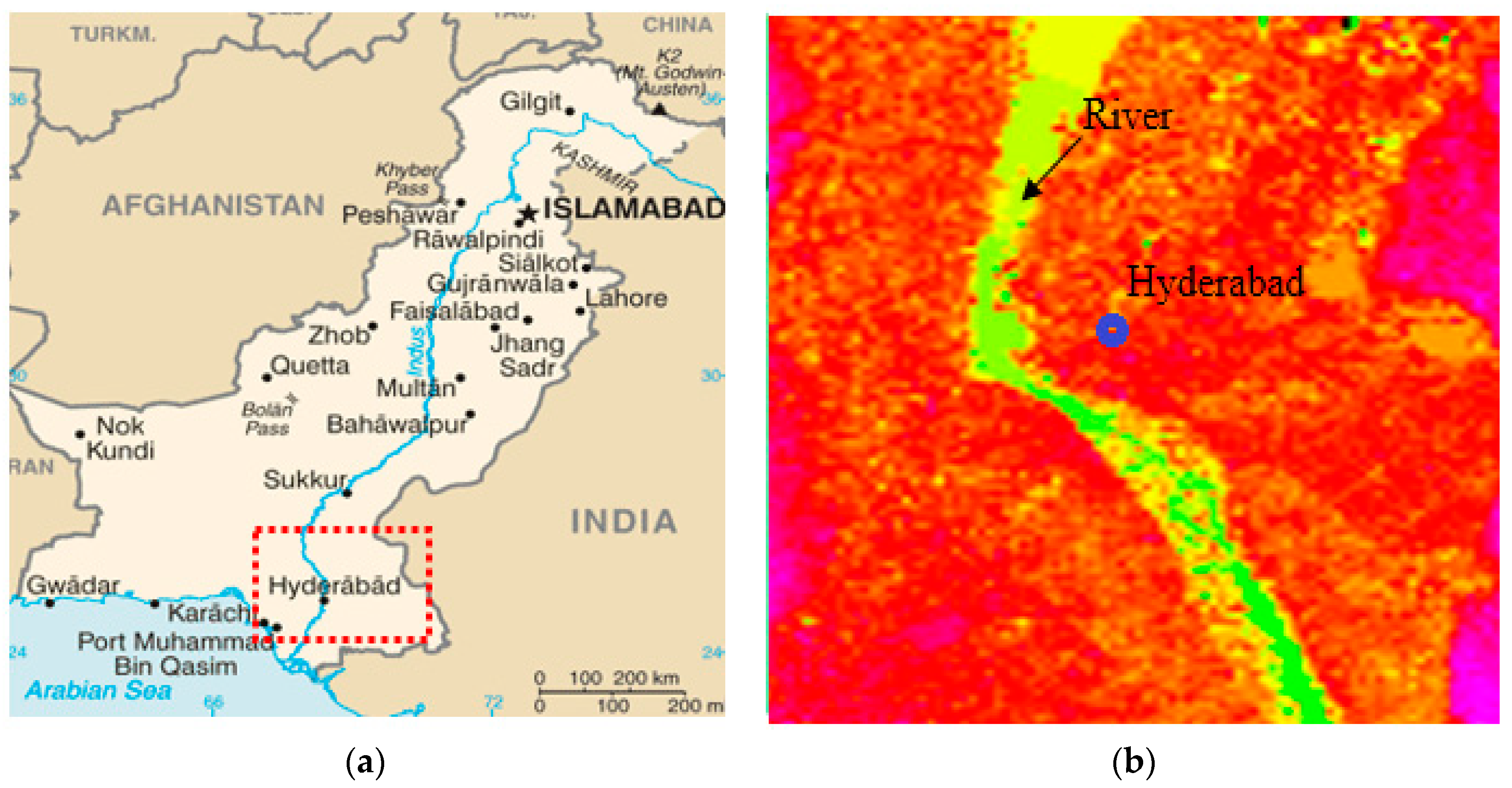
Hyderabad is the second largest city of the southeastern province in Pakistan, located at longitude 68.3578° E and latitude 25.3960° N with an elevation of 29 m. The city is part of one of the major geographical regions in Pakistan and situated at the east bank of the Indus River plain. The provincial capital Karachi is almost 150 km away, which has the largest seaport of Pakistan. The Hyderabad is considered to be in the wind corridor of Pakistan and with a good average speed virtually throughout all the seasons. The location and elevation topography view of Hyderabad city is shown in Figure 1a,b. Figure 1b shows an elevation map of the Hyderabad area. Altitudes range from 16 to 35 m, and warmer colors indicate higher altitudes. In a recent study, a Geographic Information Systems (GIS)-based map showed that areas in the southern part of Sindh province are most suitable for installing wind turbines [48].

The wind tower was installed on land with flat terrain and a wind site easily accessible by various kinds of vehicles. All instruments/sensors were tested by connecting them to the data logger before assembling to the site, and correct functioning of all the instruments during commissioning was also verified. A team of maintenance engineers and observers visited the site every month for data collection and to inspect the apparatus, and sensors were cleaned weekly. Monthly measured data were analyzed by the experts to ensure the quality of the collected wind data. The site terrain is flat with no major obstacles or roughness in the area surrounding the wind tower, except for some medium height trees and buildings with a maximum of approximately 3 m; these are about 200 m away from the tower. The coastal area and southern areas of Sindh province have land with flat terrain, with no major obstacles and roughness. Therefore, the surface roughness is between 0.03 to 0.04 m, and the roughness class for these areas is between 1.0 and 1.2 [49,50,51]. The technical specification of meteorological sensors is given in

Table 1. Specifications of meteorological sensors.

Type	Model #	Serial #	Height	Accuracy	Range
3-Cup anemometer	NRG40C	1795-00229369	10 m	±0.14 m/s at 10 m/s	1 m/s to 96 m/s
Wind direction vane	NRG200	1799-00019689	10 m	±1.6° (>0.9° to <359.1°)	0° to 360°
Temperature probe	CS215	E12267	2 m	±0.3 °C to ±0.9 °C	–40°C to +70 °C
Barometric pressure transducer	Setra 278	6015966	2 m	±0.6 to ±1.5 hPa	M 800 to 1100 hPa

. Wind speed (m/s), wind direction (degrees), atmospheric temperature (centigrade), and pressure (hPa) were measured in 10 min time intervals at the site.

3. Wind Data Analysis Procedure

Several wind characteristics such as the wind speed, the times of its occurrence, its continuity, and its direction have great significance in analyzing the wind power potential at a defined location. It is essential to have a preliminary estimate of the distribution of wind characteristics for precise feasibility of a wind farm. The total energy generation is also dependent on different factors; some of which are the air density, pressure, and turbine characteristics such as hub height and rotor diameter. Figure 2 shows a schematic diagram of the wind data analysis procedure. The two years of measured wind data were analyzed using Weibull and Rayleigh functions. Weibull parameters were estimated and used to predict different indicators for the assessment of wind power potential at the site. Wind speed for different heights was determined using the power law. Finally, the economic analysis was carried out by considering commercially available wind turbines, and mentioned aspects are discussed below.

3.1. Wind Speed Extrapolation

Measured wind speed is extrapolated, when data is collected at a limited number of heights, to determine the wind speed for multiple numbers of heights. Different methods can be used for wind extrapolation; the power law is used in this study for its simplicity. This law is considered a useful tool and is commonly used in the assessment of wind power potential to extrapolate wind speed data at different heights, which is defined as [52,53]

$$\frac{V}{V_r}={\left(\frac{Z}{Zr}\right)}^{\alpha }$$

(1)

where $V$ represents the wind speed at respective height $Z$, $V_r$ represents the wind speed at reference height $Z_r$, and $\alpha$ is the wind shear exponent. The shear exponent is a function of surface topology and varies depending on the land texture. A typical value of $\alpha$ is 1/7, which is assumed to be constant for flat terrain and low roughness surfaces. The exponent values vary from less than 0.10 for a very flat terrain, water, or ice surfaces to more than 0.25 for forest and woodlands [26,54]. The value 1/7 for $\alpha$ was considered in this study.

3.2. Weibull and Rayleigh Probability Density Functions

Various distribution functions have been used to analyze the wind data, but the two-parameter Weibull distribution is found to be the most effective [29,52,53,54,55]. Besides its many advantages, the Weibull function has a limitation: it cannot precisely represent the probabilities of zero or very low wind speeds. Therefore, a Rayleigh distribution can be used and tested, which is a special case of the two-parameter Weibull distribution function, with shape parameter k fixed at a value of 2 [26]. Probability density function and cumulative density function were used to read the wind speed variation, which indicates and compares the average speed data. The probability density function, $f\left(v\right)$, gives the probability for a given speed $v$, while the cumulative density function, $F\left(v\right)$, gives the probability for the velocity equal to or less than $v$. The Weibull probability density function (WPDF) is given as [53,54,55,56,57]

$$f\left(v\right)=\frac{k}{C}{\left(\frac{v}{C}\right)}^{k-1}\exp \left(-{\left(\frac{v}{C}\right)}^k\right)$$

(2)

where ‘$k$’ (dimensionless) and ‘$c’\left(\mathrm{m}/\mathrm{s}\right)$ represent the factor for shape and scale, respectively, which means that k and c store the complete information about the distribution.

The cumulative distribution function is the area under the curve for the probability density function. Therefore, the Weibull cumulative distribution function (WCDF), obtained by taking an integral of (WPDF), which is represented by $F\left(v\right)$, is given as

$$F\left(v\right)=1-\exp \left(-{\left(\frac{v}{C}\right)}^k\right).$$

(3)

The parameters for Weibull distribution can be calculated using various methods. Some of these are found strong while others are relatively weak. In this work, the standard deviation is used to calculate the shape and scale parameters and can be calculated as follows [29,58,59,60,61]:

$$k={\left(\frac{\sigma }{v_{avg}}\right)}^{-1.086}.$$

(4)

Moreover,

$$C=\frac{v_{avg}}{\mathsf{\Gamma }\left(1+\frac{1}{k}\right)}$$

(5)

where Γ denotes the Gamma function, which is obtained as

$$\mathsf{\Gamma }\left(x\right)={{\displaystyle \int }}_0^{\infty }{e}^{-y}{y}^{x-1}dy.$$

(6)

The scale parameter can also be computed as

$$C=\frac{v_{avg}\times k^{2.6674}}{0.184+0.816\times k^{2.73855}}.$$

(7)

Given the Weibull parameters, $C_r$ and $k_r$, at the reference height, $h_r,$ the respective parameters, $C_d$ and $k_d$, at a desired height $h_d$ is given as [60,62]

$$C_d=C_r{\left(h_d/h_r\right)}^{\beta }.$$

(8)

Moreover,

$$k_d=k_r\frac{1-0.088ln\left(h_r/10\right)}{1-0.088ln\left(h_d/10\right)}.$$

(9)

The exponent β can be calculated as

$$\beta =\frac{0.37-0.088ln\left(C_r\right)}{1-0.088ln\left(h_d/10\right)}.$$

(10)

Rayleigh distribution function (RPDF) and cumulative distribution function (RCDF) are given as follows [26,63,64]:

$$f\left(V\right)=\frac{\pi }{2}\left(\frac{V}{V^2{}_{avg}}\right)\exp \left[-\left(\frac{\mathsf{\pi }}{4}\right){\left(\frac{V}{V_{avg}}\right)}^2\right]$$

(11)

$$F\left(V\right)=1-\exp \left[-\left(\frac{\mathsf{\pi }}{4}\right){\left(\frac{V}{V_{avg}}\right)}^2\right].$$

(12)

Two other essential wind speed indicators can be calculated using Weibull parameters, which are the most probable wind speed (V_mp) and maximum energy carrying wind speed (V_maxE). Some useful numerical expressions for wind data are mentioned in Appendix A. The V_mp represents the most frequently occurred wind speed for a given distribution, whereas V_maxE is essential for considering the wind turbines for a site. After calculating shape and scale parameters, the V_mp and V_maxE can be determined by the following expressions [26,29,64]:

$$V_{mp}=C{\left(1-\raisebox{1ex}{$1$}\!\left/ \!\raisebox{-1ex}{$k$}\right.\right)}^{\frac{1}{k}}$$

(13)

$$V_{maxE}=C{\left(1+\raisebox{1ex}{$2$}\!\left/ \!\raisebox{-1ex}{$k$}\right.\right)}^{\frac{1}{k}}.$$

(14)

The most significant indicator for wind is the wind power density (WPD), which describes the quantity of energy produced by various wind speeds at a specific site. The WPD using Weibull distribution parameters can be computed as follows [63,64]:

$$WeibullWP{D}_{wb}=\frac{P_w}{A}={{\displaystyle \int }}_0^{\infty }\frac{1}{2}\rho v^{3}f\left(v\right)dv=\frac{1}{2}\rho c^3\mathsf{\Gamma }\left(1+\frac{3}{k}\right)$$

(15)

where $\rho$ is the standard air density, mostly considered a constant, 1.225 kg/m³ at sea level, a pressure of 1 atm, and a temperature of 15 °C. Air density $\left(\rho \right)$ of a month is calculated using the following equation:

$$\rho =\frac{P_{av}}{R_t\times T_{av}}$$

(16)

where $P_{av}$stands for monthly averaged air pressure in pascals. $R_t$ represents specific gas constant (287 J/kgK) for air, and $T_{av}$ refers to monthly an average temperature in Kelvin (K).

Wind power density (WPD_Ry) using Rayleigh function is calculated as follows:

$$WP{D}_{Ry}=\frac{P_w}{A}=\frac{6}{\pi }\left(\frac{1}{2}\rho V^3\right).$$

(17)

Since power density is calculated, Equations (15) and (17) can be used to estimate wind energy density (WED) for Weibull and Raleigh as follows:

$$WE{D}_{wb}=WP{D}_{wb}\times T=\frac{1}{2}\rho c^3\mathsf{\Gamma }\left(1+\frac{3}{k}\right)T.$$

(18)

Moreover,

$$WE{D}_{Ry}=WP{D}_{Ry}\times T=\frac{6}{\pi }\left(\frac{1}{2}\rho V^3\right)T.$$

(19)

Equations (18) and (19) can be used to compute WED of a particular site over a desired period T (in hours) for different wind speed frequency distributions. According to the Betz theorem, only 59.3% of wind power can be extracted using a wind turbine (WT), which is referred to as the Betz limit. By applying this limit, the probable maximum extractable power from wind is the product of the Betz limit (0.593) and the obtained results from Equation (15).

3.3. Statistical Error Analysis

In order to analyze the measured parameters, a criterion must be devised to validate the above-mentioned Weibull parameters. Errors can be computed using various statistical methods and then evaluated to find the best technique for these computations. There are different error techniques. Root mean square error (RMSE), the coefficient of determination (R²) and mean bias error (MBE) were used in this work and determined using Equations (20)–(22) [29,65]:

$$RMSE=\sqrt{\frac{1}{n}{\displaystyle \sum }_{i=1}^n{\left(y_i-x_i\right)}^2}$$

(20)

$$R^2=\frac{{{\displaystyle \sum }}_{i=1}^n{\left(y_i-m\right)}^2-{{\displaystyle \sum }}_{i=1}^n{\left(x_i-m\right)}^2}{{{\displaystyle \sum }}_{i=1}^n{\left(y_i-m\right)}^2}$$

(21)

$$MBE=\frac{1}{n}{\displaystyle \sum }_{i=1}^n\left(y_i-x_i\right).$$

(22)

where $n,y_i,x_i$ and $m$ represent observation count, actual $i^{th}$ wind speed, predicted $i^{th}$ wind speed, and the average wind speeds.

In Equations (20)–(22), all the three formulas have different characteristics. The values for these errors are positive except for the MBE. Because in the case of a good fit ${{\displaystyle \sum }}_{i=1}^n{\left(x_i-m\right)}^2$ should approach zero. Therefore, lower RMSE and MBE values and higher R² values will indicate a better fit.

3.4. Cost Assessment

It is imperative to assess the cost factor for the feasibility of wind farms in a region. The cost assessment of installing the different wind turbines was estimated using the following equations and assumptions [29,51].

Let I_c be the initial investment cost (including wind turbine cost and installation cost). Moreover, C_om is the annual operation and maintenance cost, which is 1.5–2% of wind turbine cost [29,66]. The discount operation cost for s years (the lifespan of the wind turbine) to an initial year is equal to the present cost, which can be calculated as

$$PC{(C_{om})}_{\left(1-s\right)}=n{I}_c\frac{{\left(1+r_i\right)}^s-1}{ri{\left(1+ri\right)}^s},$$

(23)

where C_om includes salary, tax, rent, and insurance. C_om can be expressed as a percentage n of I_c, while $r_i$ is the real interest rate, and s is the lifespan of the wind turbine.

Therefore, the accumulated net present cost with an effect of the initial investment cost can be obtained using the equation below:

$$NP{C}_{\left(1-s\right)}=I_c\left[1+n\left[\frac{{\left(1+r_i\right)}^s-1}{ri{\left(1+ri\right)}^s}\right]\right].$$

(24)

Similarly, the turbine annual operation cost can be obtained as

$$NPC=\frac{NP{C}_{\left(1-s\right)}}{s}=\frac{I_c}{s}\left[1+n\left[\frac{{\left(1+r_i\right)}^s-1}{ri{\left(1+ri\right)}^s}\right]\right].$$

(25)

The annual energy output of the turbine E_o can be estimated using the following equation:

$$E_o=8760\times C_f\times P_{ra}$$

(26)

where C_f is the capacity factor, and P_ra is rated the power of the turbine. Finally, the cost per kilowatt-hour of wind turbine generated electricity can be determined as follows:

$$CostofEnergy\left(COE\right)=\frac{NPC}{E_o}=\frac{I_c}{8760s}\left(\frac{1}{C_f.P_{ra}}\right)\left[1+n\left[\frac{{\left(1+r_i\right)}^s-1}{ri{\left(1+ri\right)}^s}\right]\right].$$

(27)

4. Results and Discussion

In this study, two years of wind data, from May 2015 to April 2017, collected at 10 m AGL at Hyderabad in Pakistan, were analyzed. Weibull and Rayleigh distribution functions were used to investigate the probability distribution of the wind speed data. Statistical descriptors such as the mean and standard deviations were used to compute the power and energy density for the output. Wind directions were analyzed to yield an optimum evaluation of the respective wind field. Finally, economic analysis was conducted to determine complete feasibility of the wind profile in the area. The following section is a discussion of the results obtained.

4.1. Wind Speed Analysis

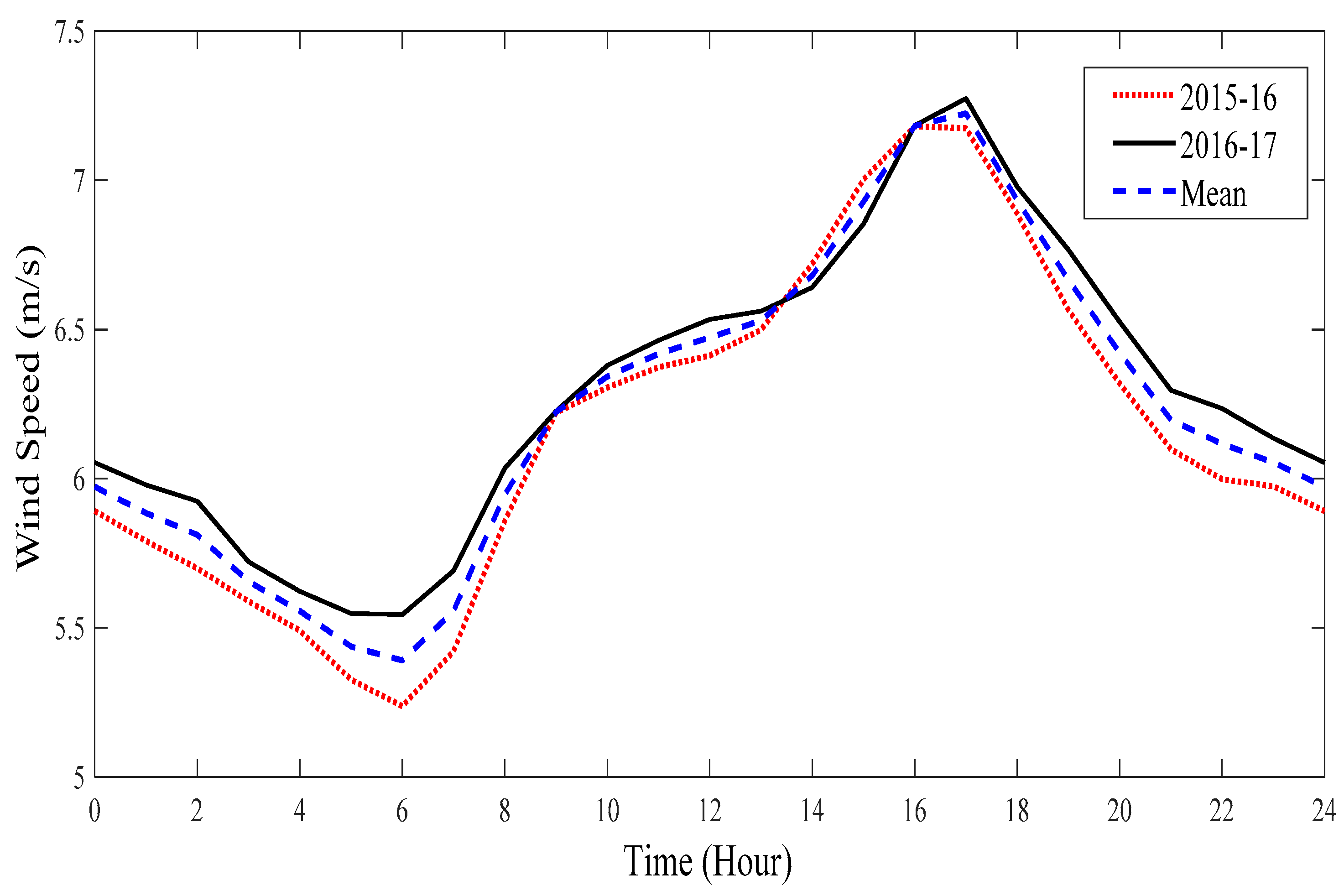
Figure 3 shows the diurnal wind speeds for the two years, 2015 to 2017, for 24 h (hourly change), and both years and mean wind speed show a consistent pattern. It can be seen that higher wind speeds occur from 7 a.m. to 6 p.m. in the daytime. The wind speeds remain above 6 m/s for more than 16 h and above 5.5 m/s all day. A maximum wind speed of 7.3 m/s was found at 5 p.m. The wind speed is relatively lower during the night and reaches a minimum of 5.2 m/s at 6 a.m., although a constant wind speed from 10 a.m. to 2 p.m. can be seen, ranging from 6 m/s to 6.5 m/s, followed by an increase to a maximum speed of 7.3 m/s, which occurs at 5 p.m. It can be seen from the graph that the average wind speed throughout the day is very steady, within a range of 6 m/s and the wind speed in the year 2016–2017 is slightly higher compared to the year 2015–2016. Figure 3 does not show the variations in the wind speed on a daily or monthly basis; this comparison is concluded in the following section.

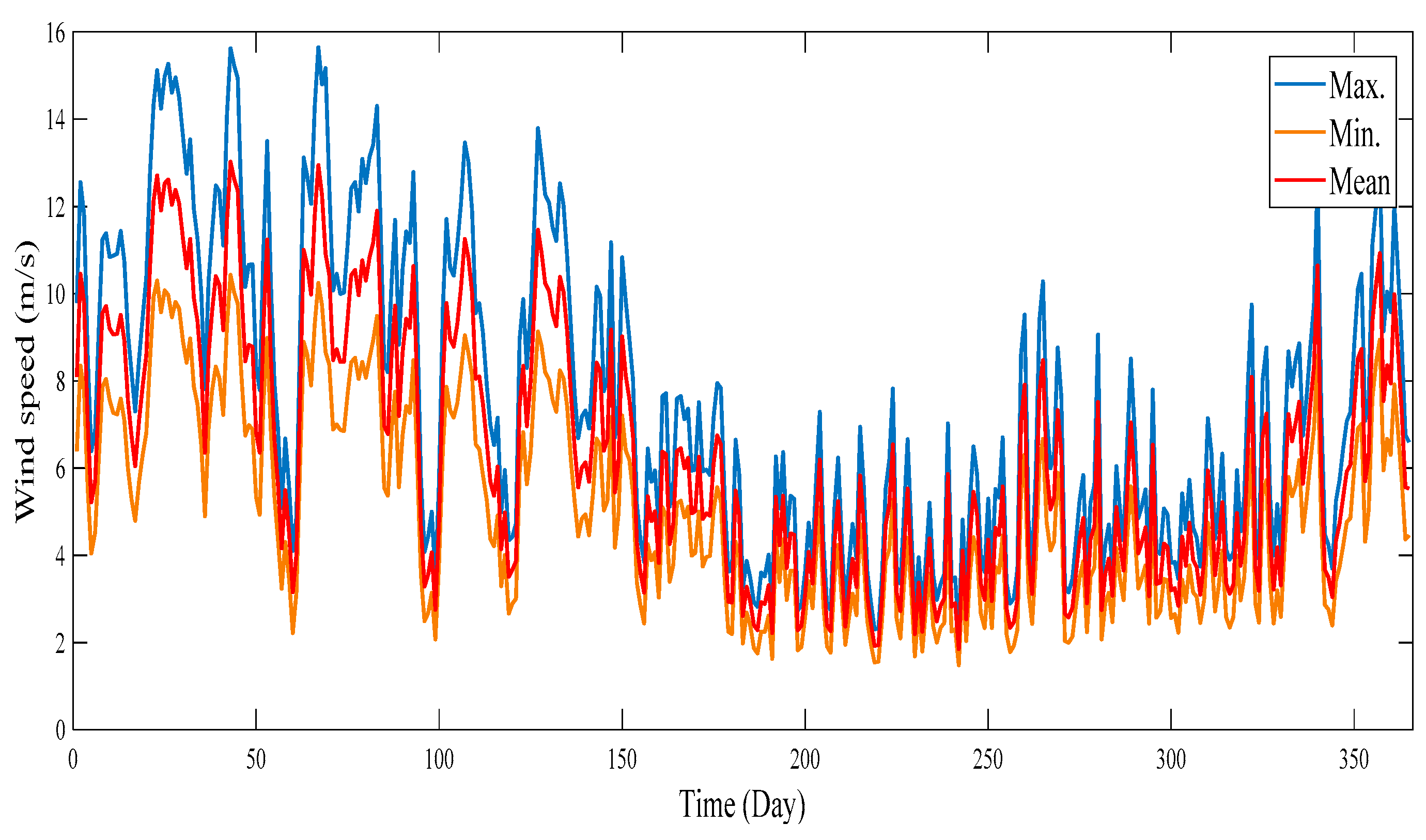
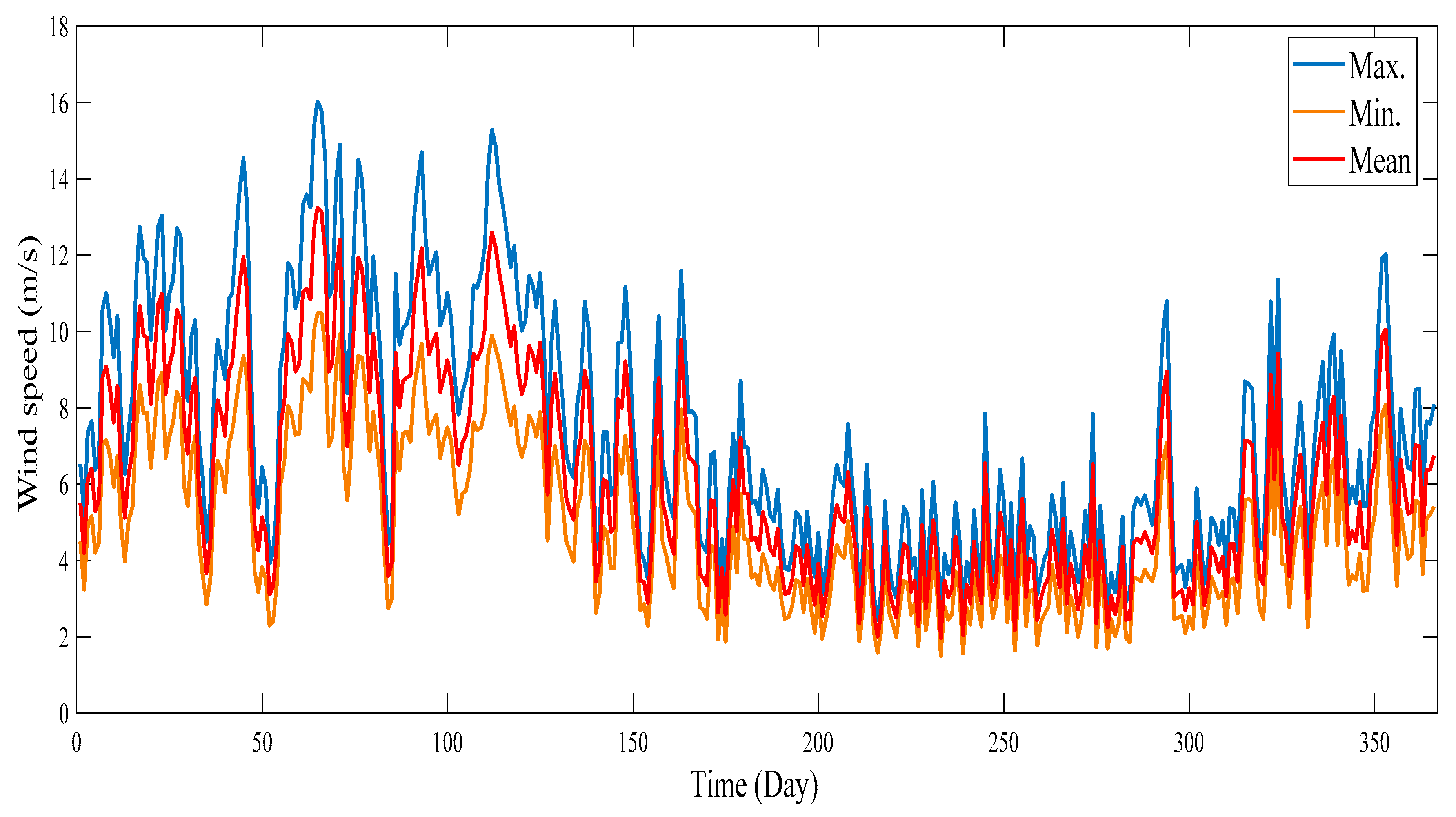
In Figure 4 and Figure 5, the averages for daily maximum and minimum wind speeds are shown along with the mean for the years 2015–2016 and 2016–2017, respectively. It can be seen that the wind speed fluctuations are very high in the mid part of both years (the data were collected from May 2015 to April 2017; Day 0 in both figures represent 1 May of the respective year), where the maximum speed increases to 16 m/s, while the minimum speed is around 2 m/s. The wind speed is comparatively steady at the end and start of the year. The minimum and maximum wind speeds range between 2 and 13 m/s for the duration of both years. As a consequence, the mean wind speed ranged from 2.5 to 10 m/s for most of the time in both years. The wind speeds of 2016–2017 follow the same pattern, impartially decreasing the maximum occurrence of wind speed to a maximum value of 15.5 m/s.

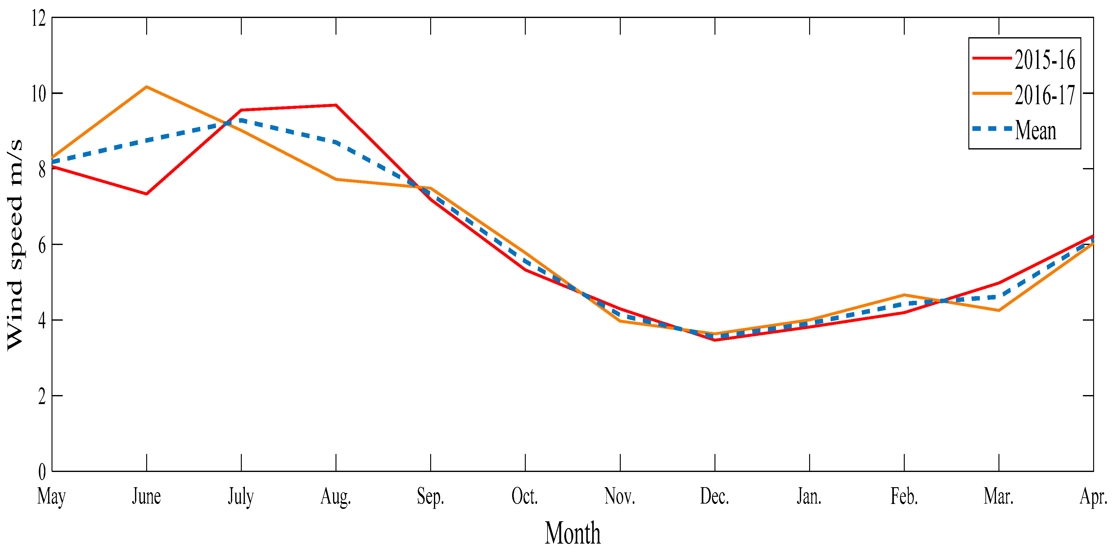
As evident from the previous analysis, the first half of the two years has higher wind speeds, while the other half shows more steady but lower wind speeds. This trend is supported by Figure 6, where monthly averaged wind speeds are shown for the two years along with their mean. The highest wind speeds were observed in August 2015 and June 2016 with values of 9.67 and 10.16 m/s, whereas the lowest was found in December for both years with values 3.46 and 3.63 m/s. Overall, the monthly average wind speed over the two years stayed between 3.5 and 10.2 m/s.

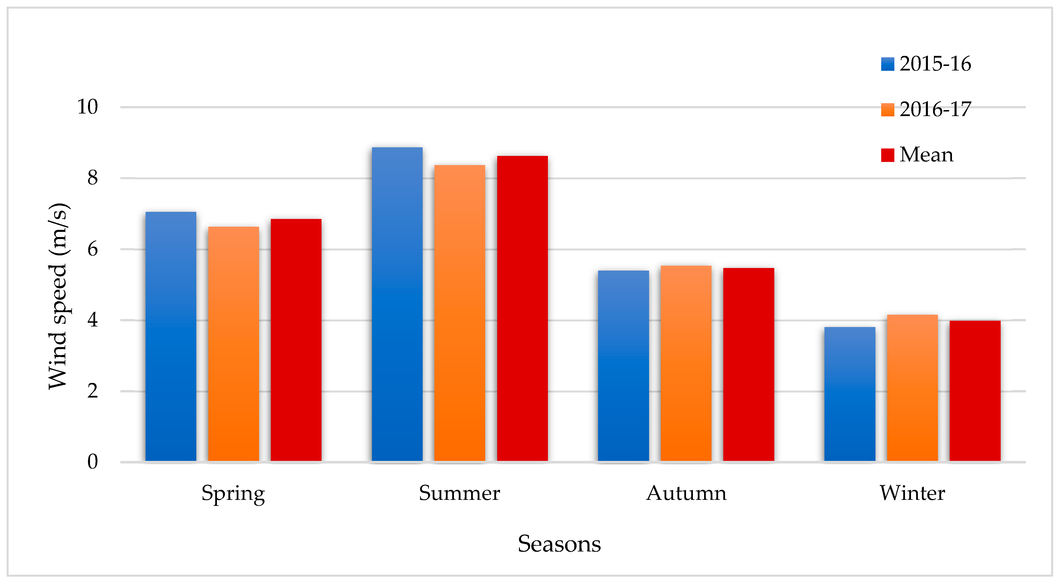
Figure 7 represents the seasonal average wind speeds for the two years and their mean of the site. The whole year is divided into four seasons: summer (from May to August), autumn (September to November), winter (December to February), and spring (March to May). It can be seen that summer is the most suitable, the highest wind speed and mean wind speed being 8.8 and 8.3 m/s for years 2015–2016 and 2016–2017, respectively, followed by spring and autumn. Winter has the lowest wind speed (approximately 4 m/s) in both years.

4.2. Wind Speed Frequency Distribution Analysis

The monthly and annual mean wind speed, standard deviation (St.dev.), turbulence intensity (Tr. I), Weibull parameters, i.e., k and c calculated using Equations (4) and (5), and specific wind characteristics (V_mp & V_maxE) of the site for both years (2015–2017) are summarized in

Table 2. Monthly and yearly mean wind, standard deviation (St. dev.), turbulence intensity (Tr. I), Weibull parameters, and specific wind characteristics for 2015–2017.

Month	Vavg (m/s)	St. dev.	Tr. I	k	c (m/s)	Vmp (m/s)	VmaxE (m/s)
May 2015	8.058	2.615	0.325	3.395	8.970	8.094	10.281
June 2015	7.331	3.012	0.411	2.627	8.251	6.876	10.235
July 2015	9.549	2.976	0.312	3.548	10.606	9.660	12.030
August 2015	9.679	2.039	0.211	5.428	10.493	10.106	11.117
September 2015	7.185	2.349	0.327	3.367	8.002	7.207	9.190
October 2015	5.324	2.358	0.443	2.421	6.005	4.819	7.700
November 2015	4.291	1.563	0.364	2.995	4.806	4.196	5.701
December 2015	3.467	1.564	0.451	2.373	3.911	3.106	5.060
January 2016	3.812	1.605	0.421	2.558	4.294	3.538	5.382
February 2016	4.195	2.184	0.521	2.031	4.734	3.391	6.635
March 2016	4.976	2.515	0.505	2.098	5.619	4.127	7.731
April 2016	6.230	2.610	0.419	2.572	7.016	5.793	8.775
May 2016	8.293	2.684	0.324	3.405	9.230	8.334	10.572
June 2016	10.164	2.463	0.242	4.662	11.115	10.554	12.000
July 2016	9.013	2.970	0.330	3.339	10.042	9.026	11.558
August 2016	7.716	2.839	0.368	2.962	8.645	7.523	10.290
September 2016	7.482	2.676	0.358	3.054	8.372	7.352	9.873
October 2016	5.774	1.979	0.343	3.199	6.447	5.734	7.504
November 2016	3.968	1.795	0.452	2.367	4.478	3.551	5.799
December 2016	3.631	1.694	0.467	2.289	4.099	3.190	5.393
January 2017	4.001	2.077	0.519	2.038	4.516	3.244	6.315
February 2017	4.662	2.191	0.470	2.271	5.263	4.076	6.951
March 2017	4.251	2.053	0.483	2.205	4.800	3.649	6.432
April 2017	6.031	2.496	0.414	2.607	6.790	5.640	8.448
Year (2015–2016)	6.269	3.117	0.497	2.136	7.078	5.266	9.646
Year (2016–2017)	6.216	3.198	0.514	2.058	7.017	5.078	9.760
Year (2015–2017)	6.242	3.158	0.506	2.097	7.050	5.172	9.703

, and seasonal measurements are shown in

Table 3. Seasonal-mean wind, standard deviation, Weibull parameters, and specific wind characteristics at 10 m height for 2015–2017.

Season	Vavg (m/s)	St. dev.	k	c (m/s)	Vmp (m/s)	VmaxE (m/s)
Summer 2015	8.853	2.919	3.336	9.864	8.865	11.355
Autumn 2015	5.600	2.437	2.468	6.314	5.115	8.030
Winter 2016	3.825	1.831	2.225	4.318	3.303	5.760
Spring 2016	6.500	2.941	2.366	7.334	5.814	9.502
Summer 2016	8.964	2.941	3.355	9.985	8.985	11.478
Autumn 2016	5.741	2.612	2.352	6.479	5.120	8.416
Winter 2016	4.098	2.043	2.129	4.627	3.436	6.315
Spring 2017	6.599	2.534	2.814	7.387	6.272	9.005

. The average value of the shape parameter for the two years is 2.097, and this parameter is almost the same for both years individually. Maximum shape parameter was in August 2015, where its value was 5.4, while the minimum was in February 2016 with a value of 2.031. The values of k for the whole data set were above 2, which indicates that the wind speed was moderate steady at a 10 m height at the candidate site. The scale parameter for the two years was 7.1 m/s, which is almost the same as that for the two years independently. The maximum scale parameter was found to be 11.115 m/s in June 2016 and 10.6 in July 2015, while the minimum was recorded to be 3.911 in December 2015 and followed by December 2016 is 4.1 m/s. The average most probable wind speed (V_mp) was found to be 5.17 m/s for the two years—6.94 m/s and 5.078 m/s for 2015–2016 and 2016–2017, respectively. The V_mp values ranged from 3.11 to 10.55 m/s. The average maximum carrying energy wind (V_maxE) of the two years was estimated at 9.703 m/s. Averages of 9.64 m/s for 2015–2016 and 9.76 m/s for 2016–2017 were found; V_maxE values ranged from 5.06 to 12.03 m/s.

The highest seasonal shape parameter k value of 3.336 was in summer 2015, and the lowest k value was in winter 2016. Seasonal scale parameter c estimates ranged from 4.318 to 8.985 m/s. The highest c value of 9.985 m/s occurred in 2016 summer and the lowest value of 4.318 m/s was in winter 2016. Seasonal V_mp values were between 3.303 and 8.985 m/s, and the highest and lowest values were 8.985 and 3.303 m/s in summer 2016 and winter 2016, respectively. The highest seasonal V_maxE value of 11.478 m/s was in summer 2016, and the lowest value was 5.760 m/s during the winter season of the year 2016.

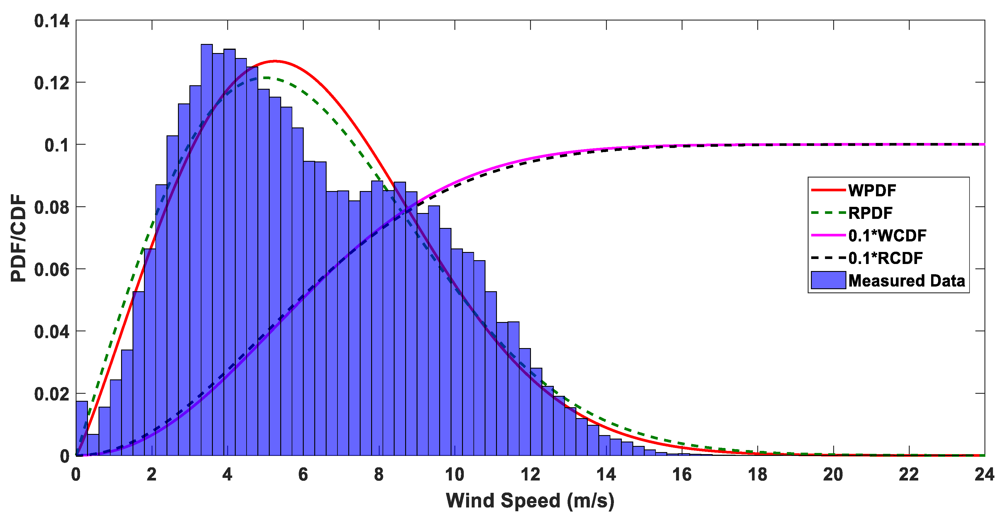
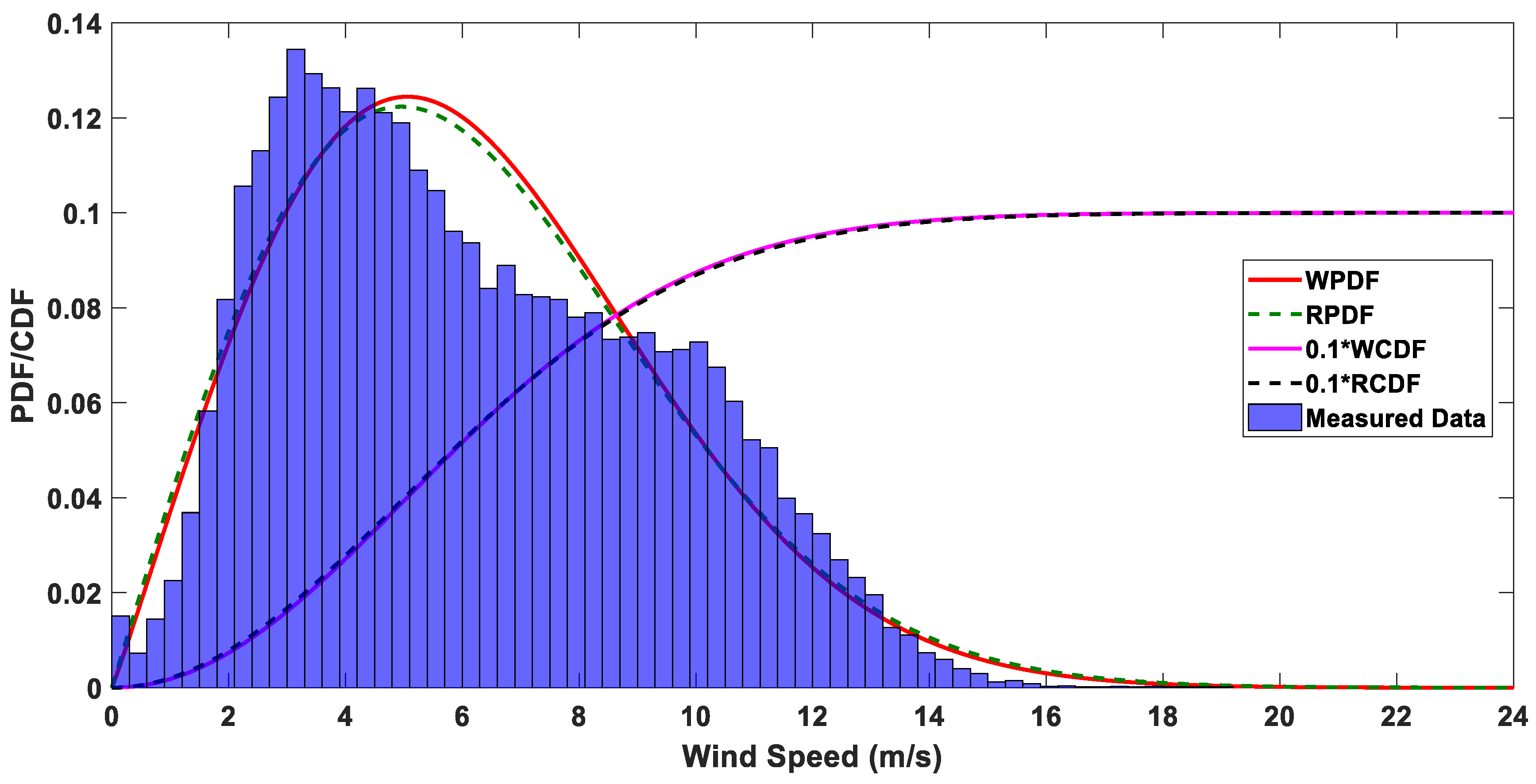
A comparison of Weibull and Rayleigh probability density functions and cumulative density functions with real data histograms is presented in Figure 8 and Figure 9 for 2015–2016 and 2016–2017, respectively. For the Rayleigh distribution, the value of k is fixed, i.e., 2. The k calculated using Equation (4) for the Weibull distribution is not constant and was found greater than 2 for both years. This trend can be seen in the related figures.

Equations (20)–(22) were used to calculate the errors and verify the accuracy of the results computed from the Weibull distribution. The errors—RMSE, R², and MBE—are given in

Table 4. Error analysis of Weibull distribution.

Years	RMSE	R2	MBE
2015–2016	0.0000760	0.9948769	0.0005121
2016–2017	0.0000747	0.9930903	0.0005590
Over all	0.0000709	0.9927871	0.0005482

. The values of all these errors are found in an acceptable range for the candidate site and verify the better fit of the Weibull distribution. Although the errors are small, the most probable wind speed was predicted to be 5 m/s by the Weibull distribution for both years, compared to around 6 m/s for the measured data.

4.3. Wind Power and Energy Density

It is significant to discuss the output generated by the wind in the form of power and energy density. The monthly values for air density ($\rho$) were calculated using Equation (16) and ranged from 1.131 to 1.205 kg/m³. The average annual $\rho$ of the proposed site was found to be 1.161 kg/m³.

Table 5. Monthly, yearly mean measured, Weibull and Rayleigh wind power density (PD_Wb), and energy density (ED_Ry).

Period	PD/(W/m2) Measured	ED/(kWh/m2) Measured	PDWb/(W/m2)	EDWb/(kWh/m2)	PDRy/(W/m2)	EDRy/(kWh/m2)
May 2015	390.17	290.29	391.02	290.92	543.54	404.40
June 2015	333.19	239.90	338.36	243.62	420.95	303.08
July 2015	626.44	466.07	637.76	474.49	897.81	667.97
August 2015	587.03	436.75	586.00	435.99	876.20	651.89
September 2015	277.80	200.01	281.25	202.50	389.97	280.78
October 2015	141.80	105.50	140.47	104.51	165.84	123.38
November 2015	65.25	46.98	65.48	47.15	86.99	62.63
December 2015	41.38	30.78	41.17	30.63	47.92	35.65
January 2016	51.64	38.42	51.78	38.53	63.40	47.17
February 2016	85.01	59.16	83.08	57.82	84.42	58.76
March 2016	136.36	101.45	131.35	97.72	137.82	102.54
April 2016	214.63	154.53	215.15	154.91	264.27	190.27
May 2016	425.89	316.86	425.08	316.26	591.42	440.02
June 2016	695.42	500.70	696.86	501.74	1030.27	741.79
July 2016	539.11	401.10	550.65	409.68	761.49	566.55
August 2016	361.18	268.71	369.81	275.14	488.92	363.76
September 2016	328.58	236.58	333.48	240.10	446.60	321.55
October 2016	151.35	112.61	150.31	111.83	204.89	152.44
November 2016	60.45	43.53	60.20	43.34	69.93	50.35
December 2016	49.11	36.53	48.10	35.79	54.46	40.52
January 2017	74.24	55.23	72.72	54.10	74.17	55.18
February 2017	106.62	71.65	103.87	69.80	116.85	78.52
March 2017	81.99	61.00	78.79	58.62	86.48	64.34
April 2017	194.05	139.72	192.71	138.75	238.64	171.82
Year (2015–2016)	255.68	2245.88	256.29	2251.29	261.92	2300.75
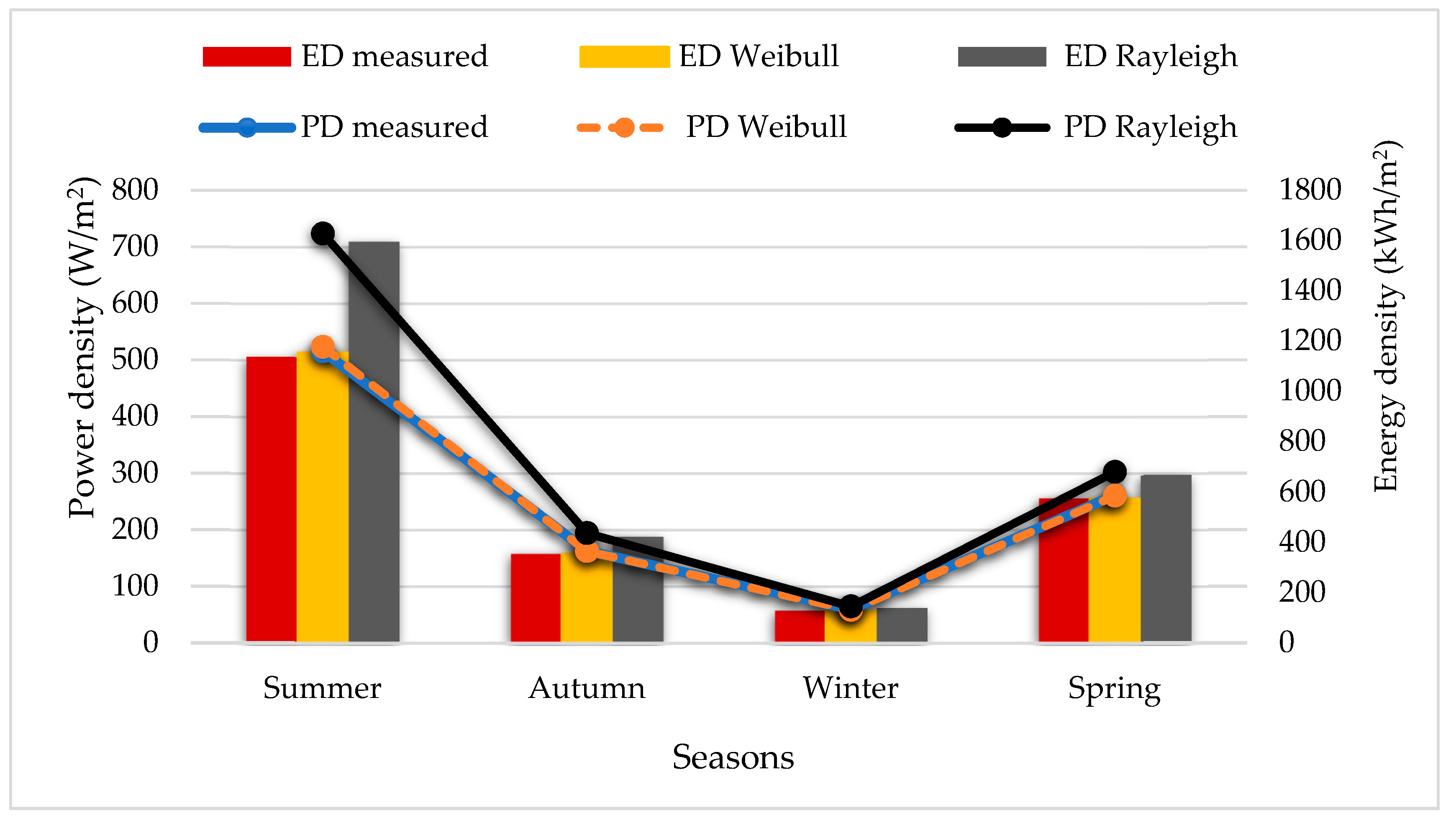
Year (2016–2017)	258.56	2265.01	259.06	2269.38	278.77	2442.01

illustrates the average monthly and yearly trends in power density and energy density calculated using the measured data and the Weibull and Rayleigh estimations. The Rayleigh function overestimates the power density for months with high wind speeds, and shows a relatively better fit for months with low wind speeds. The Weibull functions for months with low wind speeds show a slight underestimation of power density. In [21], researchers found that the Weibull function can predict the wind speed data better in comparison with the Rayleigh function. Almost similar results were found in this study, and this trend can be seen in Table 5.

For the years 2015–2016 and 2016–2017, the annual mean power density based on actual data was found to be 256.3 W/m² and 259.1 W/m², while the energy density was found to be 2245.88 kWh/m² and 2265.01 kWh/m², respectively. The monthly maximum average power density was observed to be 626.44 and 587.03 W/m² in July and August 2015 and for the year 2016–2017, and 695.42 W/m² and 539.11 W/m² in June and July 2016, respectively. The monthly minimum average power densities were 41.38 W/m² and 49.11 W/m², observed in the December of both years, whereas the highest and lowest values of energy density were found in the above-mentioned months for both years. In order to scale these outputs, the following wind classification at a 10 m height was used [29].

Fair	$P/A<100W/m^2$
Fairly good	$100\le P/A<300W/m^2$
Good	$300\le P/A<700W/m^2$
Very good	$P/A\ge 700W/m^2$

Furthermore, there is another wind power class (WPC) at 10 m height that can be used for the assessment of wind resources based on wind speed and power density [26,67]. According to this WPC, the regions classified as Class 3 or higher are considered suitable for wind power production. The calculated results of annual power density (>250 W/m²), which are given in Table 5, show that the Hyderabad area is in Class 5 and suitable for installation of wind turbines. It can be seen in Figure 10 that the higher wind speeds in the summer season resulted in a higher wind power density for both years, calculated to be more than 500 W/m². According to the defined scale for the wind power class, the summer season is in Power Class 7. The spring season is in Class 5, as the calculated power density is around 260 W/m² for both years. Finally, based on the annual estimate for the power density, the power output is relatively good for both years.

4.4. Energy Production

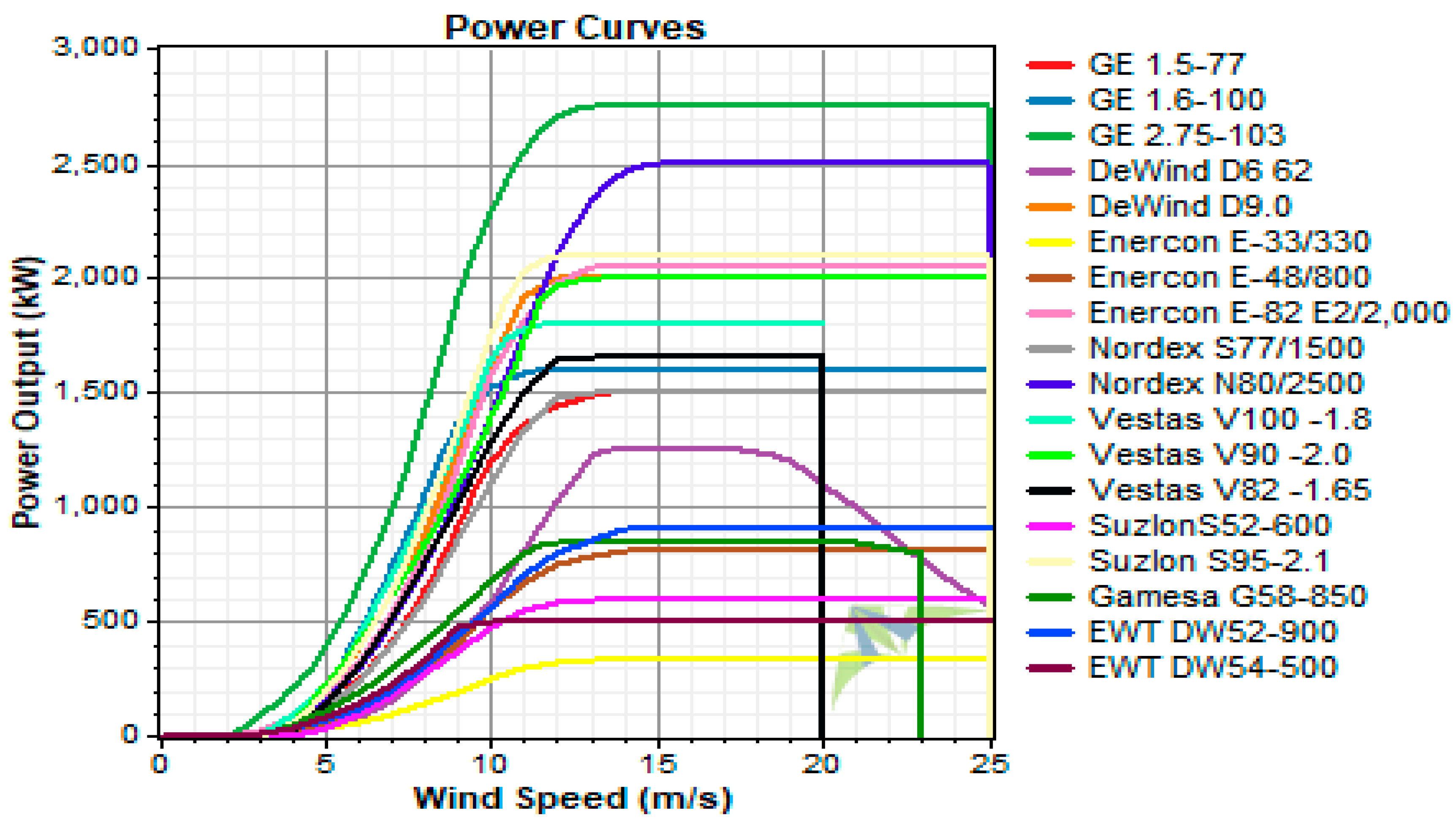
Total energy production and capacity factor are fundamental aspects of a wind power project. To determine the optimum energy output, it is essential to select the right turbine for a location. The wind data used in this research were measured at the height of the 10 m AGL. The power law was used to compute the average wind speed for different hub heights given in Equation (1). The considered hub heights were between 40 and 95 m, whereas the average wind speeds were between 7.5 and 8.5 m/s. The average wind speed was around 6.2 m/s for the whole data set, and the average maximum energy carrying wind speed (V_maxE) was about 9.7 m/s by Weibull estimation at 10 m height. The average V_maxE ranging from 9.7 to 13.4 m/s was computed up to the height of 80 m. For estimation of V_maxE at higher altitudes, the values for k and c were calculated using Equations (8) and (9). For this purpose, 18 wind energy conversion systems of different manufacturing companies (such as GE, DeWind, Enercon, Nordex, Vestas, Suzlon, and EWT DW) were selected to find the wind power, the annual energy production, and the capacity factor of the investigated site. The selected WTs’ power rating ranged from 0.33 to 2.75 MW.

The power curves of all selected WTs (curves obtained and compared using Windographer software) are shown in Figure 11 and other technical specifications are given in

Table 6. Wind turbines (WTs) technical specifications.

Turbine Model	Power Rated (MW)	Turbine Diameter (m)	Hub Height (m)
GE 1.5-77	1.5	77	65
GE 1.6-100	1.6	100	80
GE 2.75-103	2.75	103	85
DeWind D6 62	1.25	62	65
DeWind D9.0	2	93	80
Enercon E-33/330	0.33	33.4	44
Enercon E-48/800	0.8	48	55
Enercon E-82 E2/2000	2	82	85
Nordex S77/1500	1.5	77	70
Nordex N80/2500	2.5	80	80
Vestas V100-1.8	1.8	100	80
Vestas V90-2.0	2	90	95
Vestas V82-1.65	1.65	82	70
Suzlon S52-600	0.6	52	75
Suzlon S95-2.1	2.1	95	80
Gamesa G58-850	0.85	58	44
EWT DW52-900	0.9	52	50
EWT DW54-500	0.5	54	40

. To operate with its optimal capacity, the wind turbine design parameters, for example, rated power, cut out and cut in velocity, rated velocity, and hub height, were selected according to the wind characteristics of a particular site. The operating range of wind turbines was typically between 2.5 and 14 m/s, which can affect the capacity factor and cost of energy, as well as changes depending on the size of the turbine; the average maximum energy carrying wind speed (V_maxE) for this location was almost the same as the rated wind speed of the wind turbines. The power produced (P), the annual energy delivered (E), and the corresponding capacity factor using these WTs are summarized in

Table 7. WTs estimated power, annual energy output, capacity factor, and COE/MWh.

Turbine Model	P (MW)	E (MWh)	CF	$ COE/MWh
GE 1.5-77	0.668	5854.359	0.446	24.182
GE 1.6-100	0.895	7836.836	0.559	19.269
GE 2.75-103	1.282	11227.161	0.466	23.118
DeWind D6 62	0.467	4088.171	0.373	28.858
DeWind D9.0	0.976	8547.910	0.488	22.083
Enercon E-33/330	0.121	1056.818	0.366	29.471
Enercon E-48/800	0.268	2348.811	0.335	32.146
Enercon E-82 E2/2000	0.856	7495.452	0.428	25.183
Nordex S77/1500	0.679	5950.085	0.453	23.793
Nordex N80/2500	0.821	7194.369	0.329	32.796
Vestas V100 -1.8	0.970	8501.080	0.539	19.984
Vestas V90 - 2.0	0.979	8580.121	0.490	22.000
Vestas V82-1.65	0.760	6655.004	0.460	23.400
Suzlon S52-600	0.294	2579.503	0.491	21.953
Suzlon S95-2.1	1.022	8948.697	0.486	22.148
Gamesa G58-850	0.347	3043.329	0.409	26.360
EWT DW52-900	0.306	2684.490	0.340	31.642
EWT DW54-500	0.241	2107.485	0.481	22.392

. The maximum energy generated (E) per year by the GE 2.75-103 wind turbine was 11227.16 MWh followed by Suzlon S95-2.1 (8948.70 MWh) and Vestas V90-2.0 (8580.12 MWh), while the minimum energy was produced by Enercon E-33/330 (1056.82 MWh). The maximum capacity factor (CF) was 0.56 for the GE 1.6-100 wind turbine, whereas the minimum value was 0.33 for Nordex N80/2500 turbine. Overall, the selected turbines showed a good amount of energy production. Some showed a low output but still had a good CF.

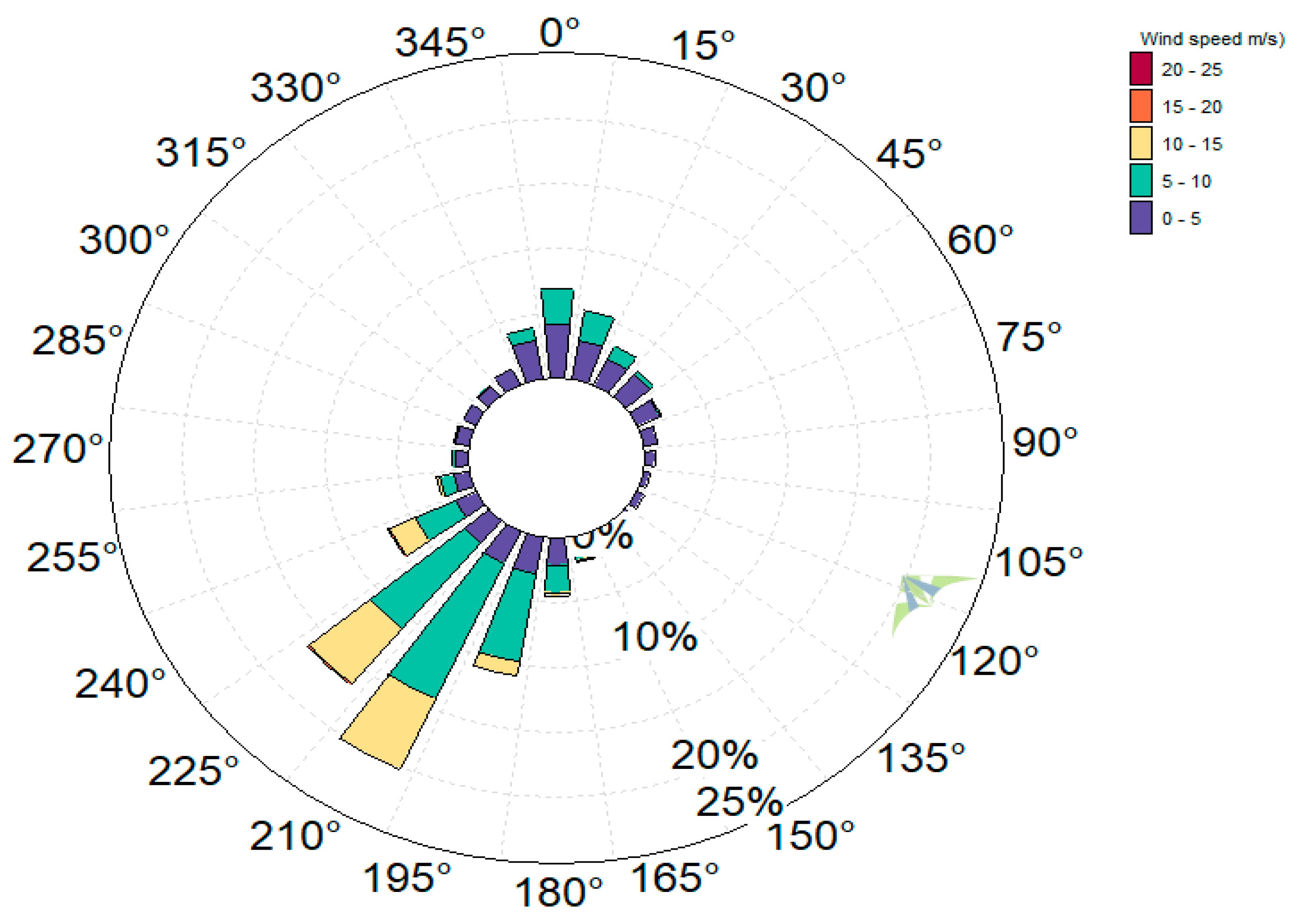
4.5. Windrose Diagrams

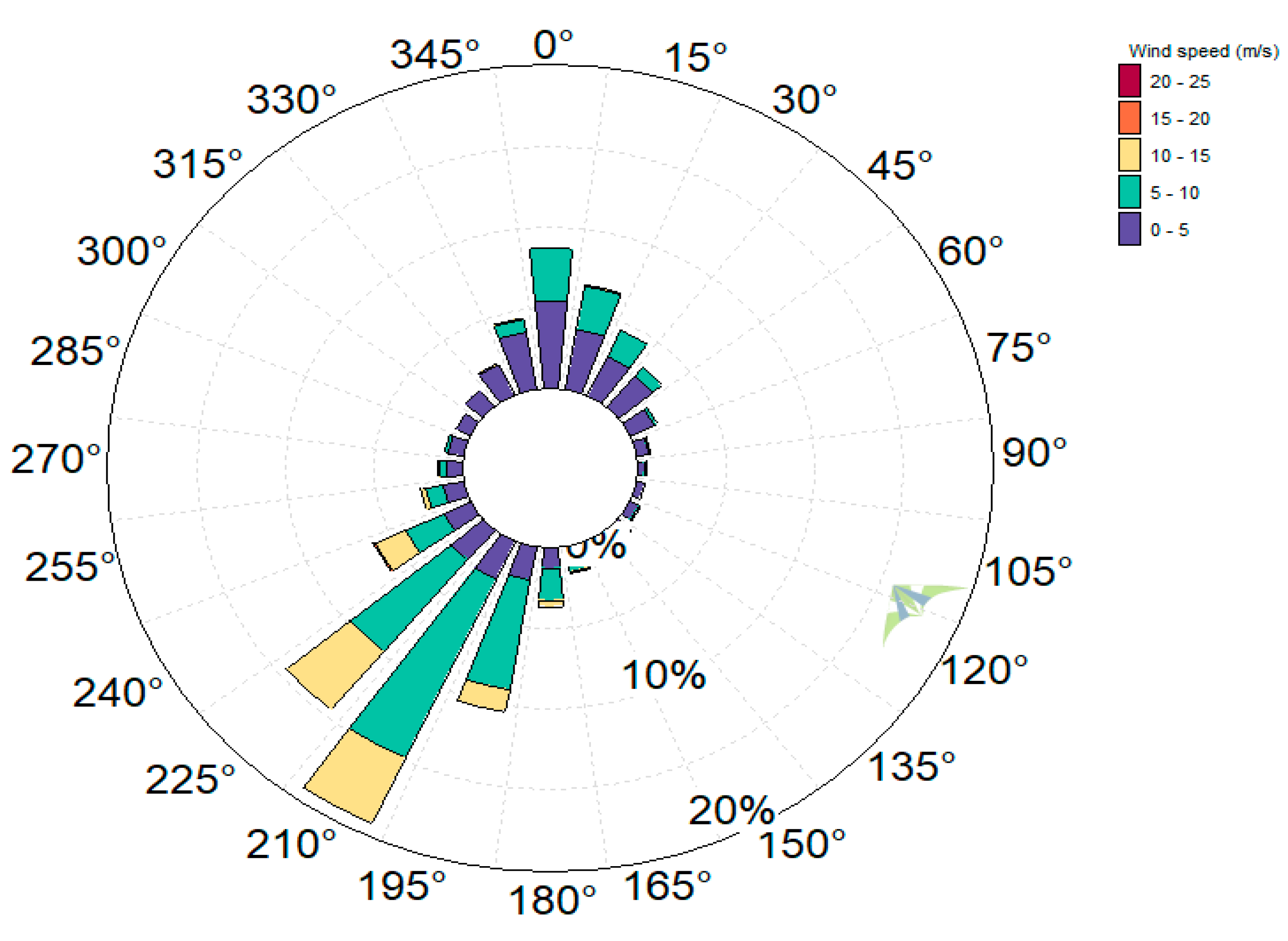
In order to determine the maximum outputs, an optimum configuration for the wind farm is required; wind direction plays an integral part in obtaining this optimization. Wind directions can be analyzed using rose diagrams, where 0° is north and a 15-degree arc divides the whole into 24 sectors. Figure 12 and Figure 13 show the average annual wind rose diagrams for the two years. Windographer was used to construct the wind rose diagram to find the overall wind direction frequency of the selected site. It can be seen from the rose graph that more than 45% of the wind is directed between 195° and 240° degrees clockwise. The critical fact is that, during the spring and summer seasons, the most productive seasons, the wind blows in the same direction.

4.6. Cost Prospect Analysis

An economic assessment of wind energy systems depends on many factors that vary in the regions. For wind energy projects, the fuel is free but requires a very high initial investment. The site is suitable for most wind turbine applications, from small standalone turbines to large wind power plants. The cost of substantial investments needed for the wind farm requires a detailed analysis of wind farm cost. Advantages and optimization of the wind farm layout are beyond the scope of this article, but an approximate economic analysis of standalone or large systems for powering the local community is described below. Wind turbines with different hub heights were selected. Hub height turbine analysis can be a benefit and provide an initial approach for the government and local investors to set up a wind farm.

The cost analysis of the selected wind turbines was calculated using Equation (27). The cost of wind turbines with power ratings above 200 kW ranged from 0.7 to 1.6 M$/MW, and an average specific cost of 1.15 M$/MW was considered [41,68]. The cost of a wind turbine in this study was estimated by assuming an initial price of 1.2 M$/MW. The initial investment cost was considered 30% of the wind turbine cost and the real interest rate was considered 10% [47]. The lifespan (s) of a wind turbine was supposed to be 20 years, whereas operation and maintenance cost were taken as 2% of the wind turbine cost [29,47]. By considering the above assumptions, the cost of energy (COE) per MW generated by the preferred wind turbines was computed, and the outcomes of these calculations are given in Table 7. To simplify the calculations, other losses, such as grid and distribution losses, transformer losses, wake losses, and cables losses were neglected and are beyond the scope of this study. The cost of energy (COE) per unit ranged from 19.27 to 32.80$/MWh. The highest cost was 32.80$/MWh for the Nordex N80/2500 wind turbine, and the lowest was 19.27$/MWh for the GE 1.6-100 wind turbine.

5. Conclusions

The wind power potential and economic analysis for electricity generation of the Hyderabad area was carried out in this research work. Two years’ worth of real-time 10-min-interval-measured wind data were analyzed to compute different indicators for the assessment of wind power potential of the proposed area. The research results indicated that the investigated site was potentially suitable for using wind energy for power generation that meets the demand for the local communities. The outcomes of this study are concluded as follows:

• The diurnal wind speed variation analysis of the site showed that higher wind speeds occurred during the daytime and reached a maximum after 5 p.m., whereas the lowest wind speeds occurred after midnight and achieved the minimum at 6 a.m. The diurnal mean wind speed remained steady throughout the two years.
• Annual average wind speed was 6.2 m/s, and the maximum mean monthly wind speeds were 10.20 m/s and 9.7 m/s in June 2016 and August 2015, respectively. Monthly average wind speed was 7.5 m/s from March to October in both years.
• Seasonal average maximum wind speeds were 8.9 m/s and 6.5 m/s in the summer and spring, respectively. The average wind speed for the winter season was 4 m/s, and for the autumn season, it was 5.6 m/s.
• Weibull shape parameter k ranged from 2.03 to 5.4 with an annual average value of 2.02. The higher values of k show that the wind speed was steady at the site. The scale parameter c ranged from 3.9 to 11.1 m/s, and the average value of an individual year was 7 m/s. The most probable wind (V_mp) and maximum energy carrying wind (V_maxE) values were in the range from 3.2 to 10.1 m/s and from 5.1 to 12. m/s respectively.
• The annual mean power density was 255 W/m², while the energy density was 2265 kWh/m². Monthly maximum average power density values were 626.44 and 587.03 W/m² for months July and August 2015 and were 695.42 and 539.11 W/m² for months June and July 2016, respectively. Monthly minimum average power densities were 41.38 and 49.11 W/m² for the December of both years. Monthly minimum average energy densities were 30.78 and 36.53 kWh/m² for the December of both years.
• RMSE, R², and MBE were found to be within an apt range for the candidate site revealing the better fitting of the distribution function.
• The annually maximum mean energy produced by the GE 2.75-103 wind turbine was 11,227.16 MWh followed by Suzlon S95-2.1 (8948.70 MWh) and Vestas V90-2.0 (8580.12 MWh), but the minimum energy was produced by the Enercon E-33/330 (1056.82 MWh) wind turbine. The maximum capacity factor (CF) was 0.56 for the GE 1.6-100 wind turbine, whereas the minimum CF was 0.33 for the Nordex N80/2500 wind turbine.
• The outcomes of the economic analysis showed that the Nordex N80/2500 wind turbine yields the highest cost of 32.80$/MWh and the GE 1.6-100 wind turbine yields the lowest cost of 19.27$/MWh, followed by Vestas V100-1.8 with a cost of 19.98$/MWh.

The findings of the study show that, for Hyderabad, wind power could be considered an alternative source of energy. The cost of energy (COE)/MWh generated by WTs is comparable to the cost of energy/MWh generated using fossil fuels. Therefore, the proposed location can be considered as a promising zone for wind power generation projects such as small standalone systems or large wind farms. Occasionally, it is not feasible to extend the main grids to small and far-flung locations. Thus, some small renewable energy resources based on standalone or off-grid power supply systems may be installed in this area to serve local communities. Further research may be directed toward selecting other types of wind turbines. Similarly, optimization of wind farm layout should also be carried out to intensify the electric power production.

References

1. Ellabban, O.; Abu-Rub, H.; Blaabjerg, F. Renewable energy resources: Current status, future prospects and their enabling technology. Renew. Sustain. Energy Rev. 2014, 39, 748–764. [Google Scholar] [CrossRef]
2. Gabbasa, M.; Sopian, K.; Yaakob, Z.; Faraji Zonooz, M.R.; Fudholi, A.; Asim, N. Review of the energy supply status for sustainable development in the Organization of Islamic Conference. Renew. Sustain. Energy Rev. 2013, 28, 18–28. [Google Scholar] [CrossRef]
3. Allouhi, A.; Zamzoum, O.; Islam, M.R.; Saidur, R.; Kousksou, T.; Jamil, A.; Derouich, A. Evaluation of wind energy potential in Morocco’s coastal regions. Renew. Sustain. Energy Rev. 2017, 72, 311–324. [Google Scholar] [CrossRef]
4. Mahela, O.P.; Shaik, A.G. Comprehensive overview of grid interfaced wind energy generation systems. Renew. Sustain. Energy Rev. 2016, 57, 260–281. [Google Scholar] [CrossRef]
5. Fazelpour, F.; Soltani, N.; Soltani, S.; Rosen, M.A. Assessment of wind energy potential and economics in the north-western Iranian cities of Tabriz and Ardabil. Renew. Sustain. Energy Rev. 2015, 45, 87–99. [Google Scholar] [CrossRef]
6. World Wind Energy Report. 2017. Available online: www.wwindea.org (accessed on 25 October 2018).
7. Global Wind Report. 2017. Available online: www.gwec.net (accessed on 28 October 2018).
8. Baloch, M.; Abro, S.; Sarwar Kaloi, G.; Mirjat, N.; Tahir, S.; Nadeem, M.; Gul, M.; Memon, Z.; Kumar, M. A research on electricity generation from wind corridors of Pakistan (two provinces): A technical proposal for remote zones. Sustainability 2017, 9, 1611. [Google Scholar] [CrossRef]
9. Jiang, H.; Wang, J.; Dong, Y.; Lu, H. Comprehensive assessment of wind resources and the low-carbon economy: An empirical study in the Alxa and Xilin Gol Leagues of inner Mongolia, China. Renew. Sustain. Energy Rev. 2015, 50, 1304–1319. [Google Scholar] [CrossRef]
10. Yaniktepe, B.; Koroglu, T.; Savrun, M.M. Investigation of wind characteristics and wind energy potential in Osmaniye, Turkey. Renew. Sustain. Energy Rev. 2013, 21, 703–711. [Google Scholar] [CrossRef]
11. Carneiro, T.C.; Melo, S.P.; Carvalho, P.C.; Braga, A.P. Particle swarm optimization method for estimation of Weibull parameters: A case study for the Brazilian northeast region. Renew. Energy 2016, 86, 751–759. [Google Scholar] [CrossRef]
12. Rocha, P.A.; de Sousa, R.C.; de Andrade, C.F.; da Silva, M.E. Comparison of seven numerical methods for determining Weibull parameters for wind energy generation in the northeast region of Brazil. Appl. Energy 2012, 89, 395–400. [Google Scholar] [CrossRef]
13. Oyedepo, S.O.; Adaramola, M.S.; Paul, S.S. Analysis of wind speed data and wind energy potential in three selected locations in south-east Nigeria. Int. J. Energy Environ. Eng. 2012, 3, 7. [Google Scholar] [CrossRef] [Green Version]
14. Arslan, T.; Bulut, Y.M.; Yavuz, A.A. Comparative study of numerical methods for determining Weibull parameters for wind energy potential. Renew. Sustain. Energy Rev. 2014, 40, 820–825. [Google Scholar] [CrossRef]
15. Wais, P. Two and three-parameter Weibull distribution in available wind power analysis. Renew. Energy 2017, 103, 15–29. [Google Scholar] [CrossRef]
16. Vogiatzis, N.; Kotti, K.; Spanomitsios, S.; Stoukides, M. Analysis of wind potential and characteristics in North Aegean, Greece. Renew. Energy 2004, 29, 1193–1208. [Google Scholar] [CrossRef]
17. Bekele, G.; Palm, B. Wind energy potential assessment at four typical locations in Ethiopia. Appl. Energy 2009, 86, 388–396. [Google Scholar] [CrossRef]
18. Kamau, J.N.; Kinyua, R.; Gathua, J.K. 6 years of wind data for Marsabit, Kenya average over 14 m/s at 100 m hub height; an analysis of the wind energy potential. Renew. Energy 2010, 35, 1298–1302. [Google Scholar] [CrossRef]
19. Sultan, A.-Y.; Charabi, Y.; Gastli, A.; Al-Alawi, S. Assessment of wind energy potential locations in Oman using data from existing weather stations. Renew. Sustain. Energy Rev. 2010, 14, 1428–1436. [Google Scholar]
20. Dahmouni, A.W.; BenSalah, M.; Askri, F.; Kerkeni, C.; BenNasrallah, S. Assessment of wind energy potential and optimal electricity generation in Borj-Cedria, Tunisia. Renew. Sustain. Energy Rev. 2011, 15, 815–820. [Google Scholar] [CrossRef]
21. Celik, A.N. Review of Turkey’s current energy status: A case study for wind energy potential of Canakkale province. Renew. Sustain. Energy Rev. 2011, 15, 2743–2749. [Google Scholar] [CrossRef]
22. Lashin, A.; Shata, A. An analysis of wind power potential in Port Said, Egypt. Renew. Sustain. Energy Rev. 2012, 16, 6660–6667. [Google Scholar] [CrossRef]
23. Mostafaeipour, A.; Sedaghat, A.; Ghalishooyan, M.; Dinpashoh, Y.; Mirhosseini, M.; Sefid, M.; Pour-Rezaei, M. Evaluation of wind energy potential as a power generation source for electricity production in Binalood, Iran. Renew. Energy 2013, 52, 222–229. [Google Scholar] [CrossRef]
24. Mostafaeipour, A.; Jadidi, M.; Mohammadi, K.; Sedaghat, A. An analysis of wind energy potential and economic evaluation in Zahedan, Iran. Renew. Sustain. Energy Rev. 2014, 30, 641–650. [Google Scholar] [CrossRef]
25. Chandel, S.S.; Ramasamy, P.; Murthy, K.S.R. Wind power potential assessment of 12 locations in western Himalayan region of India. Renew. Sustain. Energy Rev. 2014, 39, 530–545. [Google Scholar] [CrossRef]
26. Pishgar-Komleh, S.H.; Keyhani, A.; Sefeedpari, P. Wind speed and power density analysis based on Weibull and Rayleigh distributions (a case study: Firouzkooh county of Iran). Renew. Sustain. Energy Rev. 2015, 42, 313–322. [Google Scholar] [CrossRef]
27. Ammari, H.D.; Al-Rwashdeh, S.S.; Al-Najideen, M.I. Evaluation of wind energy potential and electricity generation at five locations in Jordan. Sustain. Cities Soc. 2015, 15, 135–143. [Google Scholar] [CrossRef]
28. Ozay, C.; Celiktas, M.S. Statistical analysis of wind speed using two-parameter Weibull distribution in Alaçatı region. Energy Convers. Manag. 2016, 121, 49–54. [Google Scholar] [CrossRef]
29. Fazelpour, F.; Markarian, E.; Soltani, N. Wind energy potential and economic assessment of four locations in Sistan and Balouchestan province in Iran. Renew. Energy 2017, 109, 646–667. [Google Scholar] [CrossRef]
30. Arslan, O. Technoeconomic analysis of electricity generation from wind energy in Kutahya, Turkey. Energy 2010, 35, 120–131. [Google Scholar] [CrossRef]
31. Bataineh, K.M.; Dalalah, D. Assessment of wind energy potential for selected areas in Jordan. Renew. Energy 2013, 59, 75–81. [Google Scholar] [CrossRef]
32. Ayodele, T.R.; Jimoh, A.A.; Munda, J.L.; Agee, J.T. Viability and economic analysis of wind energy resource for power generation in Johannesburg, South Africa. Int. J. Sustain. Energy 2014, 33, 284–303. [Google Scholar] [CrossRef]
33. Liu, C.; Wang, Y.; Zhu, R. Assessment of the economic potential of China’s onshore wind electricity. Resour. Conserv. Recycl. 2017, 121, 33–39. [Google Scholar] [CrossRef]
34. Aukitino, T.; Khan, M.G.; Ahmed, M.R. Wind energy resource assessment for Kiribati with a comparison of different methods of determining Weibull parameters. Energy Convers. Manag. 2017, 151, 641–660. [Google Scholar] [CrossRef]
35. Celik, A.N. A techno-economic analysis of wind energy in southern Turkey. Int. J. Green Energy 2007, 4, 233–247. [Google Scholar] [CrossRef]
36. Rehman, S.; Halawani, T.O.; Mohandes, M. Wind power cost assessment at twenty locations in the Kingdom of Saudi Arabia. Renew. Energy 2003, 28, 573–583. [Google Scholar] [CrossRef]
37. Nouni, M.R.; Mullick, S.C.; Kandpal, T.C. Techno-economics of small wind electric generator projects for decentralized power supply in India. Energy Policy 2007, 35, 2491–2506. [Google Scholar] [CrossRef]
38. Edenhofer, O.; Hirth, L.; Knopf, B.; Pahle, M.; Schlömer, S.; Schmid, E.; Ueckerdt, F. On the economics of renewable energy sources. Energy Econ. 2013, 40, S12–S23. [Google Scholar] [CrossRef]
39. Kose, F.; Aksoy, M.H.; Ozgoren, M. An assessment of wind energy potential to meet electricity demand and economic feasibility in Konya, Turkey. Int. J. Green Energy 2014, 11, 559–576. [Google Scholar] [CrossRef]
40. Fazelpour, F.; Soltani, N.; Rosen, M.A. Economic analysis of standalone hybrid energy systems for application in Tehran, Iran. Int. J. Hydrogen Energy 2016, 41, 7732–7743. [Google Scholar] [CrossRef]
41. Ayodele, T.R.; Ogunjuyigbe, A.S.O.; Amusan, T.O. Wind power utilization assessment and economic analysis of wind turbines across fifteen locations in the six geographical zones of Nigeria. J. Clean. Prod. 2016, 129, 341–349. [Google Scholar] [CrossRef]
42. Khahro, S.F.; Soomro, A.M.; Tabbassum, K.; Dong, L.; Liao, X. Assessment of wind power potential at Hawksbay, Karachi Sindh, Pakistan. Indones. J. Electr. Eng. Comput. Sci. 2013, 11, 3479–3490. [Google Scholar] [CrossRef]
43. Aman, M.M.; Jasmon, G.B.; Ghufran, A.; Bakar, A.H.; Mokhlis, H. Investigating possible wind energy potential to meet the power shortage in Karachi. Renew. Sustain. Energy Rev. 2013, 18, 528–542. [Google Scholar] [CrossRef]
44. Ullah, I.; Chipperfield, A.J. An evaluation of wind energy potential at Kati Bandar, Pakistan. Renew. Sustain. Energy Rev. 2010, 14, 856–861. [Google Scholar] [CrossRef]
45. Mirza, I.A.; Khan, N.A.; Memon, N. Development of benchmark wind speed for Gharo and Jhimpir, Pakistan. Renew. Energy 2010, 35, 576–582. [Google Scholar] [CrossRef]
46. Wind Power Potential at Jamshoro-Sindh; Pakistan Meteorological Department. Available online: www.pmd.gov.pk/wind/Sindh/Jamshoro.pdf (accessed on 22 October 2018).
47. Khahro, S.F.; Tabbassum, K.; Soomro, A.M.; Dong, L.; Liao, X. Evaluation of wind power production prospective and Weibull parameter estimation methods for Babaurband, Sindh Pakistan. Energy Convers. Manag. 2014, 78, 956–967. [Google Scholar] [CrossRef]
48. Jamshed, A.; Saleem, A.A.; Javed, S.; Riffat, M. Site Suitability Analysis for Developing Wind Farms in Pakistan: A GIS-Based Multi-Criteria Modeling Approach. Sci. Technol. Dev. 2018, 37, 195–201. [Google Scholar]
49. Wind Data Investigation Reports. Available online: www.aedb.org (accessed on 16 January 2019).
50. AEDB Pakistan. Wind Data Analysis of AEDB-UNDP (WEP) Wind Mast. Available online: http://climateinfo.pk/frontend/web/attachments/datatype/AEDB_UNDP%20(2010)%20Analysis%20of%20Data%20of%20Wind%20Masts%20in%20Gharo-Keti%20Bandar%20Wind%20Corridor.pdf (accessed on 16 January 2019).
51. Khahro, S.F.; Tabbassum, K.; Soomro, A.M.; Liao, X.; Alvi, M.B.; Dong, L.; Manzoor, M.F. Techno-economical evaluation of wind energy potential and analysis of power generation from wind at Gharo, Sindh Pakistan. Renew. Sustain. Energy Rev. 2014, 35, 460–474. [Google Scholar] [CrossRef]
52. Manwell, J.F.; McGowan, J.G.; Rogers, A.L. Wind Energy Explained: Theory, Design and Application; John Wiley & Sons: Chichester, UK, 2010. [Google Scholar]
53. Albani, A.; Ibrahim, M.Z. Wind energy potential and power law indexes assessment for selected near-coastal sites in Malaysia. Energies 2017, 10, 307. [Google Scholar] [CrossRef]
54. Islam, M.R.; Saidur, R.; Rahim, N.A. Assessment of wind energy potentiality at Kudat and Labuan, Malaysia using Weibull distribution function. Energy 2011, 36, 985–992. [Google Scholar] [CrossRef]
55. Akdag, S.A.; Bagiorgas, H.S.; Mihalakakou, G. Use of two-component Weibull mixtures in the analysis of wind speed in the Eastern Mediterranean. Appl. Energy 2010, 87, 2566–2573. [Google Scholar] [CrossRef]
56. Pang, W.-K.; Forster, J.J.; Troutt, M.D. Estimation of wind speed distribution using Markov chain Monte Carlo techniques. J. Appl. Meteorol. 2001, 40, 1476–1484. [Google Scholar] [CrossRef]
57. Chang, T.P. Performance comparison of six numerical methods in estimating Weibull parameters for wind energy application. Appl. Energy 2011, 88, 272–282. [Google Scholar] [CrossRef]
58. Carta, J.A.; Ramirez, P. Analysis of two-component mixture Weibull statistics for estimation of wind speed distributions. Renew. Energy 2007, 32, 518–531. [Google Scholar] [CrossRef]
59. Manyeredzi, T.; Makaka, G. An Assessment of the Wind Power Generation Potential of Built Environment Wind Turbine (BEWT) Systems in Fort Beaufort, South Africa. Sustainability 2018, 10, 1346. [Google Scholar] [CrossRef]
60. Justus, C.G.; Hargraves, W.R.; Mikhail, A.; Graber, D. Methods for estimating wind speed frequency distributions. J. Appl. Meteorol. 1978, 17, 350–353. [Google Scholar] [CrossRef]
61. Balouktsis, A.; Chassapis, D.; Karapantsios, T.D. A nomogram method for estimating the energy produced by wind turbine generators. Sol. Energy 2002, 72, 251–259. [Google Scholar] [CrossRef]
62. Kang, D.; Ko, K.; Huh, J. Comparative Study of Different Methods for Estimating Weibull Parameters: A Case Study on Jeju Island, South Korea. Energies 2018, 11, 356. [Google Scholar] [CrossRef]
63. Celik, A.N. A statistical analysis of wind power density based on the Weibull and Rayleigh models at the southern region of Turkey. Renew. Energy 2004, 29, 593–604. [Google Scholar] [CrossRef]
64. Keyhani, A.; Ghasemi-Varnamkhasti, M.; Khanali, M.; Abbaszadeh, R. An assessment of wind energy potential as a power generation source in the capital of Iran, Tehran. Energy 2010, 35, 188–201. [Google Scholar] [CrossRef]
65. Mohammadi, K.; Alavi, O.; Mostafaeipour, A.; Goudarzi, N.; Jalilvand, M. Assessing different parameters estimation methods of Weibull distribution to compute wind power density. Energy Convers. Manag. 2016, 108, 322–335. [Google Scholar] [CrossRef]
66. Mathew, S. Wind Energy: Fundamentals, Resource Analysis and Economic; Springer: Berlin, Germany, 2006; Volume 1. [Google Scholar]
67. NRC. Wind Power Class. Available online: https://www.nrc.gov/docs/ML0720/ML072040340.pdf (accessed on 17 February 2019).
68. Gökçek, M.; Genç, M.S. Evaluation of electricity generation and energy cost of wind energy conversion systems (WECSs) in Central Turkey. Appl. Energy 2009, 86, 2731–2739. [Google Scholar] [CrossRef]
Figure 1. Hyderabad city overview: (a) location, (b) elevation topography.
Sustainability 11 01391 g001
Figure 2. Schematic diagram for wind data analysis procedure.
Sustainability 11 01391 g002
Figure 3. Diurnal wind speed variations for 2015–2017.
Sustainability 11 01391 g003
Figure 4. Daily maximum, minimum, and mean wind speed variations for 2015–2016.
Sustainability 11 01391 g004
Figure 5. Daily maximum, minimum, and mean wind speed variations for 2016–2017.
Sustainability 11 01391 g005
Figure 6. Monthly mean wind speed variations for 2015–2017.
Sustainability 11 01391 g006
Figure 7. Seasonal-mean wind speeds for year (2015–2017).
Sustainability 11 01391 g007
Figure 8. Wind speed frequency distribution analysis for 2015–2016.
Sustainability 11 01391 g008
Figure 9. Wind speed frequency distribution analysis for 2016–2017.
Sustainability 11 01391 g009
Figure 10. Seasonal wind power and energy density from summer 2015 to spring 2017.
Sustainability 11 01391 g010
Figure 11. Power curves of selected wind turbines.
Sustainability 11 01391 g011
Figure 12. Windrose diagram for the year 2015–2016.
Sustainability 11 01391 g012
Figure 13. Windrose diagram for the year 2016–2017.
Sustainability 11 01391 g013