A Multi-Objective and Multi-Dimensional Optimization Scheduling Method Using a Hybrid Evolutionary Algorithms with a Sectional Encoding Mode

Abstract

Aimed at the problem of the green scheduling problem with automated guided vehicles (AGVs) in flexible manufacturing systems (FMS), the multi-objective and multi-dimensional optimal scheduling process is defined while considering energy consumption and multi-function of machines. The process is a complex and combinational process, considering this characteristic, a mathematical model was developed and integrated with evolutionary algorithms (EAs), which includes a sectional encoding genetic algorithm (SE-GA), sectional encoding discrete particle swarm optimization (SE-DPSO) and hybrid sectional encoding genetic algorithm and discrete particle swarm optimization (H-SE-GA-DPSO). In the model, the encoding of the algorithms was divided into three segments for different optimization dimensions with the objective of minimizing the makespan and energy consumption of machines and the number of AGVs. The sectional encoding described the sequence of operations of related jobs, the matching relation between transfer tasks and AGVs (AGV-task), and the matching relation between operations and machines (operation-machine) respectively for multi-dimensional optimization scheduling. The effectiveness of the proposed three EAs was verified by a typical experiment. Besides, in the experiment, a comparison among SE-GA, SE-DPSO, H-SE-GA-DPSO, hybrid genetic algorithm and particle swarm optimization (H-GA-PSO) and a tabu search algorithm (TSA) was performed. In H-GA-PSO and TSA, the former just takes the sequence of operations into account, and the latter takes both the sequence of operations and the AGV-task into account. According to the result of the comparison, the superiority of H-SE-GA-DPSO over the other algorithms was proved.

1. Introduction

With the development of the manufacturing industry and the changes of the competitive market, meeting customer’s diverse demands and improving service quality has become the main direction of shifting their strategy for manufacturing enterprises, and flexible manufacturing system (FMS) become an effective way to meet these needs. At the same time, intelligent manufacturing has become a major trend in the development of manufacturing [1,2,3]. Under the background, FMS provides great flexibility for the intelligent manufacturing workshop and plays more and more important roles in intelligent manufacturing, especially to meet concurrent production of various parts on one or more pieces of large equipment. An FMS consists of material handling devices (automated guided vehicles (AGVs) and robots), workstations, automated storage systems, and so on. An AGV is an automatic transport vehicle, which can navigate along a planned route with different guidance ways and systems [4]. It is widely used to transfer material in modern production systems and enhance the efficiency of it [5,6,7]; all AGVs can have unified scheduling using a central computer control system so that all shop floor operations would be controlled through an AGVs system.

AGVs scheduling of FMS is an important problem, which can affect the productivity, delivery cost and service quality to a great extent; it also determines the efficiency of the whole production system [8]. In most of the existing studies, the sequence of operation of related jobs and the matching relation between transfer tasks and AGVs (AGV-task) are the main ways to optimize the AGV scheduling problem; they are two related dimensions, which are important and effective in AGV scheduling [9]. Deroussi et al. proposed a solution method for the simultaneous scheduling for the sequence of operation and allocation of AGVs [10]. Lacomme et al. introduced a framework based on a disjunctive graph to model the joint scheduling problem of machines and AGVs [11]. Baruwa et al. proposed a simultaneous scheduling method of machines and AGVs based on a timed colored petri net approach [12]. Besides, there are also some practical conditions in the workshop that have been taken into consideration by researchers in their studies, such as battery charging of AGVs, cost of operation, time of operation, and so on [13,14,15,16]. Cai et al. developed a mixed regional control model for production tasks to solve the problem of task scheduling and coordination control presented by a multi-AGV system [17]. Novas et al. proposed a novel approach by taking resource-constraints, the loaded and the empty movements of the device, into account [18]. Mchaney proposed several methods that can be used to account for the impact of various battery usage schemes on AGV simulations [19]. Kabir et al. investigated how the duration of battery charging for AGVs can be varied to increase flexibility and manufacturing capacities of a manufacturing system [20]. Yan et al. investigated the capability to evaluate reliability issues in AGVs by considering the health management of these vehicles and their optimal mission configuration [21]. Although a lot of studies has been carried out for AGV scheduling by building different models, there are also some other conditions that need to be considered for further optimization of AGVs scheduling. In FMS, a lot of machines are versatile; it means that a single machine can process multiple operations and has different processing capabilities for different operations. Therefore, it is useful to optimize machine selection in the process of manufacturing by optimization of AGV scheduling. A similar problem has been studied by many researchers for manufacturing resource combinatorial optimization (MRCO) [22,23,24,25] and has provided important references for the optimization of machine selection in FMS by AGVs.

In the aspect of optimization objectives of AGVs scheduling in FMS, earlier studies have mainly concentrated on minimizing the makespan of all related jobs, and have been effectively applied on increasing productivity and the resource utilization rate [8,15,16]. Sometimes, the makespan is presented in the form of the travel distance of all AGVs [26]. Caridá et al. proposed a method for AGV scheduling in FMS using fuzzy systems with the objective of minimizing the makespan [27]. Chang et al. proposed a hybrid genetic algorithm (HGA) to improve the makespan solution for the distributed FMS scheduling problem [28]. Achmad et al. proposed a non-dominated sorting biogeography-based optimization (NSBBO) scheduling method in FMS with the objective of minimizing the makespan problem and total earliness [29]. However, as one of the most important parts in FMS, the number of them heavily influences the profitability in an FMS and increasing the utilization rate of AGVs is important for optimizing the performance of the FMS [30,31,32]. Some studies have been carried out to meet the demand for better optimal scheduling of AGVs in FMS. Mousavi et al. proposed an optimal scheduling model for AGVs that the objectives of which are the minimization of the makespan and number of AGVs while considering the AGVs battery charge; two optimization algorithms were also developed in the model [15,16]. Vivaldini et al. presented a methodology for the estimation of the minimum number of AGVs required to execute a given transportation order within a specific time-window [33]. With the development of green manufacturing, studies have been done for a green workshop by considering the energy consumption of the machines, which is also an important running cost [34,35,36]. Therefore, the energy consumption of the machines should be one of the objectives of AGV scheduling in FMS to reduce the cost and optimize the manufacturing quality, which few have taken into account.

In summary, although a lot of effective studies have been done on the AGV scheduling problem in FMS, there is still value and a need for further research into the two problems as follows:

(1) It is of great value for enterprises to take more objectives such as energy consumption of machines into account for synthetically optimizing the manufacturing process and benefit the FMS.

(2) In FMS, optimizing the sequence of operations and the matching relation between transfer tasks and AGVs are just two dimensions to improve the performance of the production system, but, as we know, many machines have a variety of process capabilities, and optimizing machine selection should be an important part for increasing the resource utilization rate and the productivity in FMS.

To address the above concerns, this research developed a multi-objective and multi-dimensional optimization scheduling mathematical model while considering energy consumption and multi-function of the machines. In the model, the multi-objective is to minimize the makespan and energy consumption of the machines and the number of AGVs; the multi-dimensional objective is to simultaneously optimize the sequence of operation of related jobs, the matching relation between transfer tasks and AGVs (AGV-task) and the matching relation between operations and machines (operation-machine) for the multi-objective. To solve this kind of problem, evolutionary algorithms (EAs) are the common methods [9,37,38,39]. Some distinct research in the scheduling context that can also provide some new ideas for FMS with AGVs [40,41,42]. The model proposed in this research will be optimized in three-dimensions, as mentioned earlier using three evolutionary algorithms (sectional encoding genetic algorithm (SE-GA), sectional encoding discrete particle swarm optimization (SE-DPSO) and hybrid sectional encoding genetic algorithm and discrete particle swarm optimization (H-SE-GA-DPSO)) and the corresponding experiments and a comparison among them are introduced. Besides, the hybrid genetic algorithm, particle swarm optimization (H-GA-PSO) and tabu search algorithm (TSA) are also applied for the comparison; the former just takes the sequence of operation into account, which is proposed in literature [15], and the latter takes both the sequence of operation and AGV-tasks into account, which is proposed in literature [9].

The rest of this paper is organized as follows. The model, problem description and assumptions are detailed in Section 2. The algorithm design is explained in Section 3. The experiment and discussion are presented to verify the effectiveness of the algorithms proposed in this paper in Section 4. Especially, a comparison among results SE-GA, SE-DPSO, H-SE-GA-DPSO, H-GA-PSO and TSA is provided to prove the superiority of H-SE-GA-DPSO. Finally, Section 5 provides the conclusion of this paper and indicates the research direction to a further extent.

2. Problem Description and Mathematical Model

2.1. Problem Description

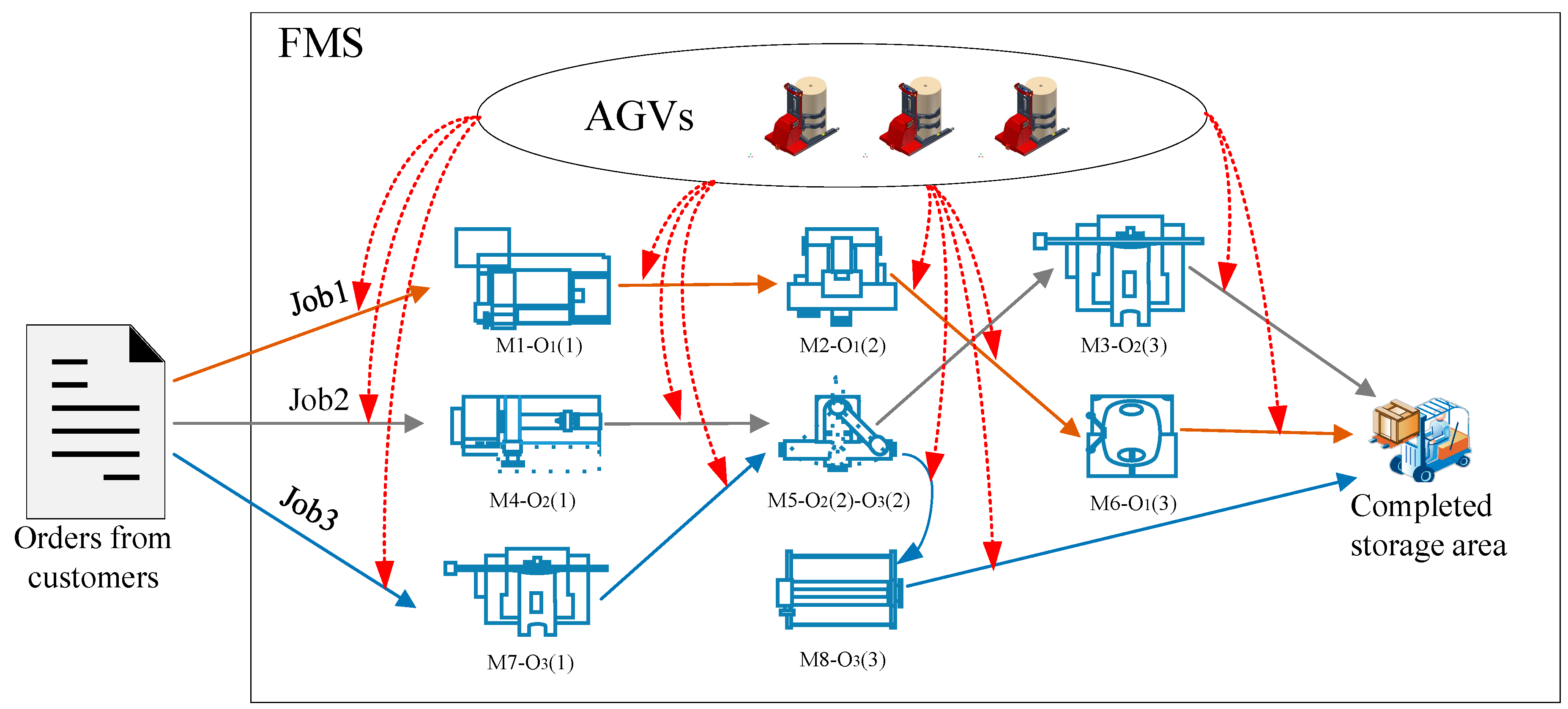
On the basis of the current AGV multi-objective optimization scheduling problems in FMS, a multi-objective and multi-dimensional scheduling model of AGVs is presented in this paper, as shown in Figure 1. Let us assume that there are several jobs assigned to an FMS, which can be described as a set of jobs {J₁, J₂, ..., J_n}. Each of the jobs contains several operations. For instance, J_i is composed of the sequence of operations {O_i(1), O_i(2), ..., O_i(m_i)}. Some of the related machines {M₁, M₂, ..., M_s} in this FMS are selected to execute these operations with limited AGVs {A₁, A₂, ..., A_t}, and each of them can meet one or more of the operations {O_a(b), O_c(d), ..., O_e(f)}. The same operation can be executed by different machines with different energy consumption. Therefore, the corresponding candidate machines for O_i(j) are marked as {M_x, M_y, ..., M_z}. In this model, the operating time and energy consumption of each operation executed on each candidate machine, standby energy consumption of each machine per unit time, logistics time among all machines are pre-known. The assumptions in the model are as follows:

• All AGVs have a unit-load capacity.
• There are no battery charge problems on any AGV.
• AGVs and machines operate continuously without breakdown.
• There are no traffic problems, collision, deadlock.
• AGV loading and unloading times are fixed and considered as travel times.
• AGVs can always park at their unloading locations.
• The velocity of AGVs is constant.
• The start point (SP) of each job is in the home position (H) of the AGV.
• The machine-to-machine distances and SP-to-machine distances are known.
• Each machine operates only one product at a time.
• The setup times are included in the time of production.

To formulate the mathematical model of the problem, the related parameters and variables are summarized in the Appendix A attached to this paper.

2.2. Mathematical Model

Three objects, which include the makespan, energy consumption and the number of AGVs are taken into account in the mathematical model. It can be formulated as follows.

Minimizing the makespan. The mathematical expression of the makespan (MS) can be expressed by:

$$\begin{array}{ll}\mathit{MS}& =\mathit{max}\{{\mathit{MFT}}_k\}=\mathit{max}\{{\mathit{AFT}}_l+T({k,N}_k)\}=\mathit{max}\{\mathit{ot}(i)\}\\ & =\mathit{max}\{\mathit{tt}(i)+\mathit{ot}({i,m}_i)\}\end{array}$$

(1)

$$MF{T}_k={\displaystyle \sum _{p=1}^{N_k}(T(k,p)+WT(k,p))}$$

(2)

$$AF{T}_l={\displaystyle \sum _{q=1}^{N_l}(T(l,q)+WT(l,q))}$$

(3)

$$ot(i)=o{t}_s(i,1)+{\displaystyle \sum _{j=1}^{m_i}(ot(i,j)+otw(i,j))}$$

(4)

$$tt(i)=t{t}_s(i,1)+{\displaystyle \sum _{j=1}^{m_i}(tt(i,j)+ttw(i,j))}$$

(5)

$$WT(k,p)=T_s(k,p)-T_e(k,p-1)$$

(6)

$$WT(l,q)=T_s(l,q)-T_e(l,q-1)$$

(7)

$$otw(i,j)=o{t}_s(i,j)-o{t}_e(i,j-1)$$

(8)

$$ttw(i,j)=t{t}_s(i,j)-t{t}_e(i,j-1)$$

(9)

$$\begin{array}{l}ot(i,j),T(k,p)=o{t}_e(i,j)-o{t}_s(i,j),\\ \mathrm{if}{O}_i(j)\mathrm{is}\mathrm{assigned}\mathrm{to}M(k)\mathrm{and}\mathrm{index}\mathrm{of}\mathrm{it}\mathrm{for}M(k)\mathrm{is}p\end{array}$$

(10)

$$\begin{array}{l}tt(i,j),T(l,q)=t{t}_e(i,j)-t{t}_s(i,j),\\ \mathrm{if}T{A}_{ij}\mathrm{is}\mathrm{assigned}\mathrm{to}\mathrm{AGV}l\mathrm{and}\mathrm{index}\mathrm{of}\mathrm{it}\mathrm{for}\mathrm{AGV}l\mathrm{is}q\end{array}$$

(11)

Subject to:

$$MS\le DT$$

(12)

$${\displaystyle \sum _{i=1}^n{m}_i={\displaystyle \sum _{k=1}^s{N}_k}}$$

(13)

$${\displaystyle \sum _{i=1}^n{m}_i={\displaystyle \sum _{l=1}^t{N}_l}}.$$

(14)

Here, Equation (1) defines the calculation method of MS, which can be represented by the maximum finish time of the operations assigned to each machine (i.e., max{MFT_k}), the maximum finish time of traveling tasks assigned to each AGV (i.e., max{AFT_l+T(k,N_k)}), the maximum finish time of operations of each job (i.e., max{ot(i)}) or the maximum finish time of traveling for each job (i.e., max{tt(i)+ot(i,m_i)}). Equations (2) and (6) define the calculation method of related values, which determine the result of max{MFT_k}. Equations (3) and (7) define the calculation method of related values which determines the result of max{AFT_l+T(k,N_k)}. Equations (4), (8) and (10) define the calculation method of related values, which determines the result of max{ot(i)}. Equations (5), (9) and (11) define the calculation method of related values, which determines the result of max{tt(i)+ot(i,m_i)}.

Constraint number (12) ensures the feasibility of completion time by meeting the demand of DT. Constraint numbers (13) and (14) define the numerical relationship of m_i, N_k and N_l in Equations (1)–(5).

Minimizing energy consumption. The mathematical expression of energy consumption can be expressed by:

$$ES=esw+ese$$

(15)

$$esw={\displaystyle \sum _{k=1}^{s}esw(k)}={\displaystyle \sum _{k=1}^s{\displaystyle \sum _{p=1}^{N_k}WT(k,p)}}\times wesu(k)={\displaystyle \sum _{i=1}^n{\displaystyle \sum _{j=1}^{m_i}otw(i,j)}}\times wesu(k)$$

(16)

$$ese={\displaystyle \sum _{k=1}^{s}ese(k)={\displaystyle \sum _{k=1}^s{\displaystyle \sum _{p=1}^{N_k}es(k,p)}}}={\displaystyle \sum _{i=1}^n{\displaystyle \sum _{j=1}^{m_i}es(i,j)}}.$$

(17)

Here, Equation (15) defines the ES of all machines by completing all jobs. Equations (16) and (17) define the calculation methods of esw and ese, which compose ES. In Equation (16), otw(i,j)×wesu(k) means the M_k is chosen to executing the operation number j of job number i.

Minimizing the number of AGVs. The number of AGVs is denoted by NA. Generally, more AGVs means a smaller makespan while it also means increased costs. Therefore, it is important to minimize the number of AGVs to optimize the performance of the FMS.

Multi-objective evaluation. The decision is usually made by considering a comprehensive result when there are several objectives that have to be taken into account. Pareto has given an effective method for us to solve multi-objective optimization problems. In the method, Pareto-optimal set and Pareto-front refer to a group of best trade-off schedules and a set of Pareto solutions respectively [15]. The overall fitness function formulation for the three objectives is described by:

$$f(x)={\phi }_1{f}_1(x)+{\psi }_1{\phi }_2{f}_2(x)+{\psi }_2{\phi }_3{f}_3(x)$$

(18)

$${\phi }_1+{\phi }_2+{\phi }_3=1{\phi }_1>0,{\phi }_2>0,{\phi }_3>0.$$

(19)

φ₁, φ₂ and φ₃ are the weights of three objectives respectively and they are constrained by Equation (19). f₁(x), f₂(x) and f₃(x) in Equation (18) correspond to the fitness functions of the three objectives. Therefore, the overall fitness function is described by:

$$f(x)={\phi }_{1}MS+{\psi }_1{\phi }_{2}ES+{\psi }_2(1-{\phi }_1-{\phi }_2)NA.$$

(20)

ψ₁ and ψ₂ in Equation (18) are the ratios to balance among the objectives with different ranges of value [41]. To facilitate the calculation and analysis by considering the main part of the ES and NA, they are defined by:

$${\psi }_1=\frac{DT}{max(ese)}$$

(21)

$${\psi }_2=\frac{DT}{max(NA)}.$$

(22)

The expression max(ese) in Equation (21) is the maximum energy consumption by completing the operation of all jobs.

3. Algorithm Design

The genetic algorithm (GA) and particle swarm optimization (PSO) are the most typical evolutionary algorithms (EAs) to solve AGV scheduling problems. The GA is a search algorithm based on the mechanics of the natural selection process. It has the capability of simultaneous evaluation of many points in the search area, which increases the probability of finding the global solution to the problem [15]. Besides, the encoding method of the GA is very flexible [43,44,45,46], and it can be used to solve different types of problems using a suitable encoding format. PSO is a population EA, which is inspired by social behavior of bird flocking; this kind of algorithm makes use of the population wisdom to search cooperatively so as to find the optimal result in the solution space. Compared with other algorithms, it is more robust as it can work with limited information such as the fitness evaluation of each particle [47]. The encoding method of PSO can meet the continuous and discrete variable values, therefore, it can be used to solve both the extremum approximation and MRCO problems [48,49]. To improve the performance of the algorithms, hybrid EAs have also been studied in a lot of research by integrating the advantages of the compensatory properties of each algorithm to obtain better results [50,51,52].

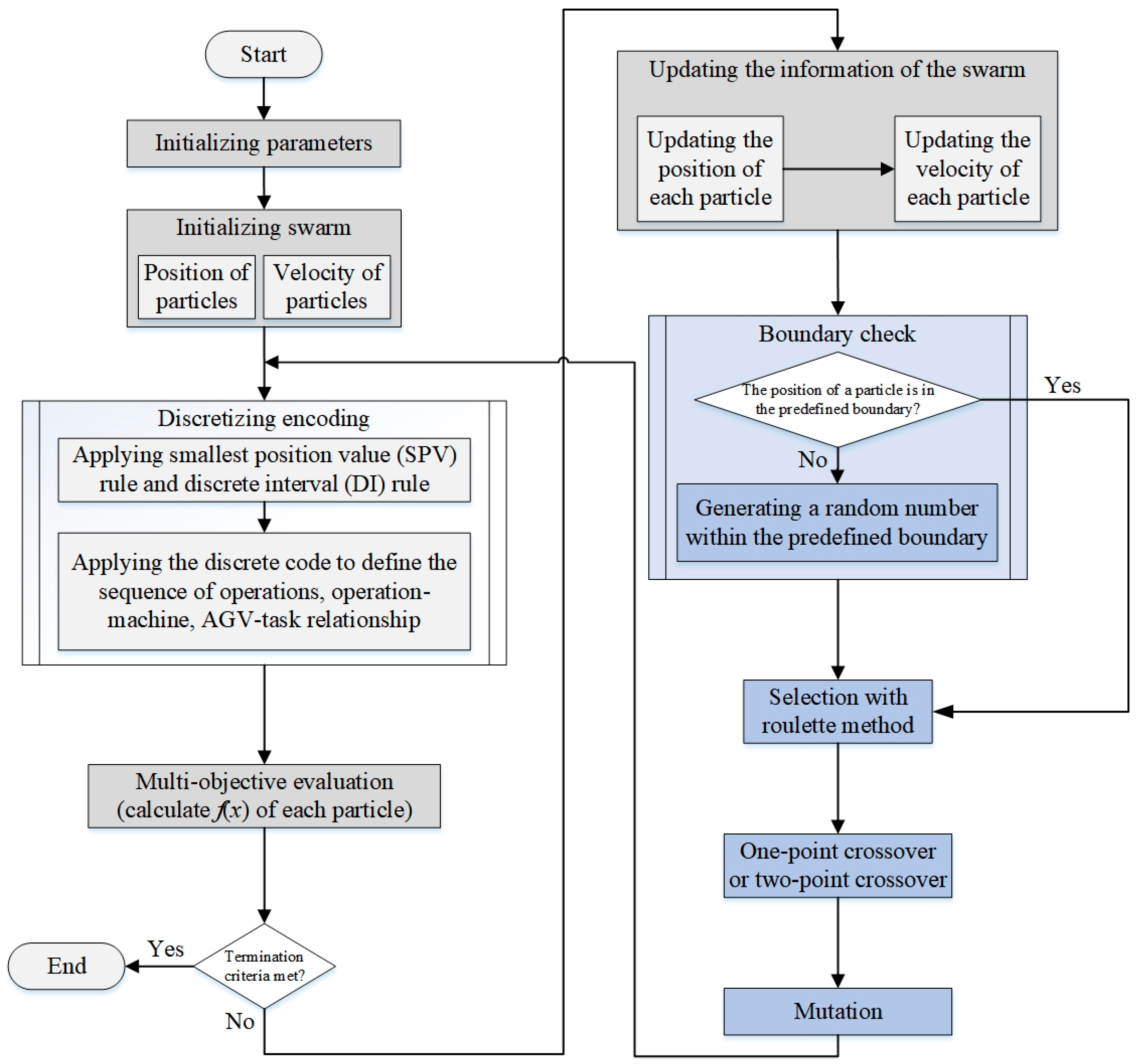
On this basis, a hybrid sectional encoding genetic algorithm and discrete particle swarm optimization (H-SE-GA-DPSO) have been developed to meet the model proposed in this paper. It is a hybrid algorithm, which has the characteristics of the genetic algorithm and particle swarm optimization. In the algorithm, both the chromosome encoding and particle encoding are divided into three segments for multi-dimensional optimization scheduling. Correspondingly, sectional encoding genetic algorithm (SE-GA), sectional encoding discrete particle swarm optimization (SE-DPSO), hybrid genetic algorithm and particle swarm optimization (H-GA-PSO) and a tabu search algorithm (TSA) are also proposed and compared with H-SE-GA-DPSO. Here, H-GA-PSO has been proven to be a more effective algorithm in optimizing the sequence of operations [15]. Besides, as two related dimensions, both the sequence of operation and AGV-tasks have been taken into account for further optimization in studies by TSA [9]. The related steps and configurations of SE-GA and SE-DPSO respectively are shown in Section 3.1 and Section 3.2. Figure 2 illustrates the flowchart of H-SE-GA-DPSO, which is explained in detail in Section 3.1 and Section 3.2.

3.1. Sectional Encoding Genetic Algorithm

The sectional encoding genetic algorithm (SE-GA) is the main algorithm of the proposed H-SE-GA-DPSO; it can also provide optimized solutions independently. The basis of it is the GA; the difference is that the chromosome encoding it is divided into three segments for multi-dimensional optimization scheduling. Therefore, the main steps of it are similar to the GA that can be described as follows:

Step 1. Initializing parameters. It involves setting the crossover rate (CR), the mutation rate (MR), population size (PS), length of a chromosome (LC), the maximum number of iterations (NC_max), related basic data and so on.

Table 1. General schematic for reading data.

SE-GA (C1)	Chromosome (Cr)						Operations (Oi(j))
	SgSo		SgOm		SgAt
	Gene Number (Ge)	Gene Code (g)	Gene Number (Ge)	Gene Code (g)	Gene Number (Ge)	Gene Code (g)
	G1	1	Gθ+1	1	G2θ+1	1	O1(1)
	G2	1	Gθ+2	3	G2θ+2	3	O1(2)
		…	…	…	…	…	…
	Gm1	1	Gθ+m1	2	G2θ+m1	2	O1(m1)
		2		s		5	O2(1)
		…		…		…	…
		2		5		4	O2(m2)
		…		…		…	…
		n		k		NA	On(1)
		…		…		…	…
	Gθ	n	G2θ	4	G3θ	l	On(mn)
SE-DPSO (P1)	Particle (Pr)						Operations (Oi(j))
	SgSo		SgOm		SgAt
	Dimension Number (dn)	Dimension Code (dc)	Code of Dimension (dc)
	1	2	1		1		O1(1)
	2	3	3		3		O1(2)
	…	…	…		…		…
	m1	c	2		2		O1(m1)
	…	…	s		5		O2(1)
			…		…		…
			5		4		O2(m2)
		θ	…		…		…
		…	k		NA		On(1)
			…		…		…
	θ	1	4		l		On(mn)

shows the data structure for the model proposed in this research. The column ‘Gene code(g)’ of ‘SgSo’, the column ‘Gene code(g)’ of ‘SgOm’ and the column ‘Gene code(g)’ of ‘SgAt’ show the code of the segment of sequence of operations (SgSo), segment of operation-machine (SgOm), segment of AGV-task (SgAt) of a chromosome (C_r) respectively, which will be discussed later.

Step 2. Initializing population. A set of chromosomes will be generated in this step.

Chromosome encoding. The encoding used in this paper is real number coding according to the needs of the problem. As shown in the column ‘Gene code(g)’ of ‘SgSo’ of Table 1, each gene code defines an operation related to a job. The order of genes represents the priority of operations, which decreases from left to right. In the column ‘Gene code(g)’ of ‘SgOm’, each gene code defines a machine to execute an operation. Different from SgSo, the order of it is fixed according to the original sequence of operations. In the column ‘Gene code(g)’ of ‘SgAt’, each gene code defines an AGV to execute a traveling task. The order of it is the same with SgOm.

A chromosome (C_r) is expressed by:

$$\begin{array}{ll}{C}_r& =\{(O_i(j)),(M_i(j),(A_i(j)))|i=1,2,\dots ,n,j=1,2,\dots ,m_i\}\\ & =\{\{\underset{\theta }{\underbrace{O_2(1),O_1(2),\dots ,O_i(j),\dots ,O_n(m_n),\dots ,O_i(m_i)}}\},\\ & \hspace{1em}\{(\underset{m_1}{\underbrace{M_1(1),M_1(2),\dots ,M_1(m_1)}}),(\underset{m_2}{\underbrace{M_2(1),M_2(2),\dots ,M_2(m_2)}}),\dots ,(\underset{m_n}{\underbrace{M_n(1),M_n(2),\dots ,M_n(m_n)}})\},\\ & \hspace{1em}\{(\underset{m_1}{\underbrace{A_1(1),A_1(2),\dots ,A_1(m_1)}}),(\underset{m_2}{\underbrace{A_2(1),A_2(2),\dots ,A_2(m_2)}}),\dots ,(\underset{m_n}{\underbrace{A_n(1),A_n(2),\dots ,A_n(m_n)}})\}\}\end{array}$$

(23)

It meets the conditions as follows:

$${\displaystyle \sum _{i=1}^n{m}_i=\theta }.$$

(24)

The length of a chromosome is expressed by:

$$LC=3*\theta .$$

(25)

Chromosome coding is explained by an example of three jobs (J₁, J₂, J₃), and each job has two, two, and three operations respectively, and C_r is a random construct of $\left[\underset{\mathrm{SgSo}}{\underbrace{2312331}}\underset{\mathrm{SgOm}}{\underbrace{\underset{J_1}{\underbrace{21}}\underset{J_2}{\underbrace{43}}\underset{J_3}{\underbrace{532}}}}\underset{\mathrm{SgAt}}{\underbrace{\underset{J_1}{\underbrace{13}}\underset{J_2}{\underbrace{21}}\underset{J_3}{\underbrace{123}}}}\right]$. Here, in part of the SgSo, code ‘1’, ‘2’, and ‘3’ imply operations of J₁, J₂, and J₃ respectively, and from the left, the first ‘1’ represents the first operation of J₁, the second ‘1’ represents the second operation of J₁, the first ‘2’ represents the first operation of J₂, and so on. In part of the SgOm, from the left, the first ‘2’ represents the first operation of J₁, executed by machine number 2. The first ‘1’ represents the second operation of J_1, executed by machine number 1. The first ‘4’ represents the first operation of J₂, executed by machine number 4, and so on. In part of the SgAt, from the left, the first ‘1’ means that the traveling task of the first operation of J₁ is executed by AGV number 1. The second ‘3’ means that the traveling task of the second operation of J₁ is executed by AGV number 3 and so on.

Step 3. Fitness evaluation. Each chromosome is evaluated by the makespan, energy consumption and number of AGVs in accordance with Equations (1) to (17). In addition, the total fitness values were calculated based on Equations (20) to (22).

Step 4. Generating a new population. A new population is generated by selection, crossover, and mutation operation.

Selection. The roulette method, which is a probability random selection method, was used in this study for the selection operator.

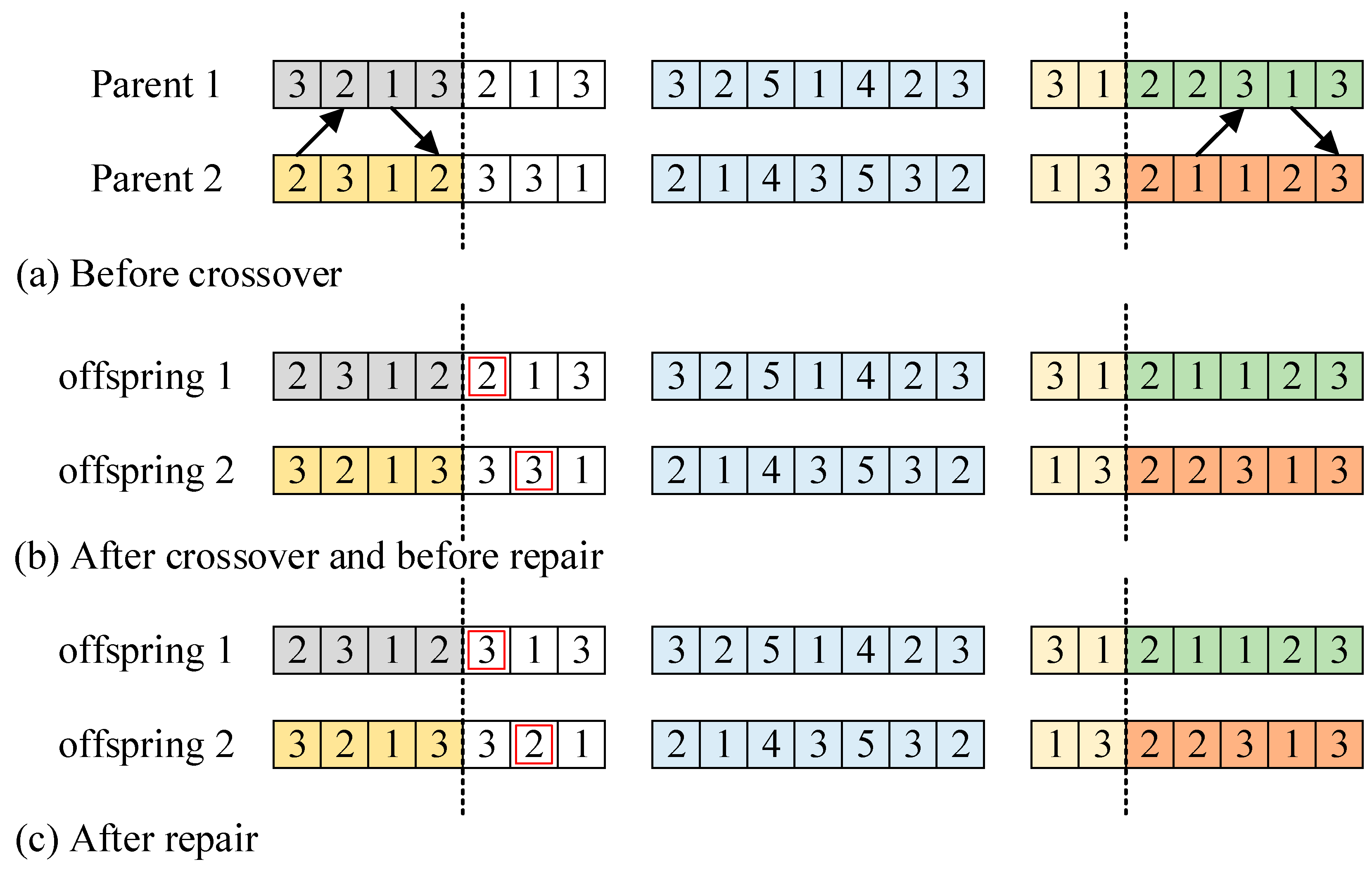
Crossover. A one-point crossover and a two-point crossover based on a partial string exchange were employed, where the two-point crossover is illustrated in Figure 3a,b based on the example in step 2. The offspring generated by the crossover may be an illegal encoding. For example, the uncorrected code of the operation of a job may be seen in part of the SgSo. Therefore, these illegal SgSo codes should be repaired as shown in Figure 3.

The number of crossovers is calculated by:

$$Numberofcrossovers=\frac{CR\times PS}{2}.$$

(26)

Mutation. The number of mutations in each generation is calculated by:

$$Numberofmutations\cong PS\times MR.$$

(27)

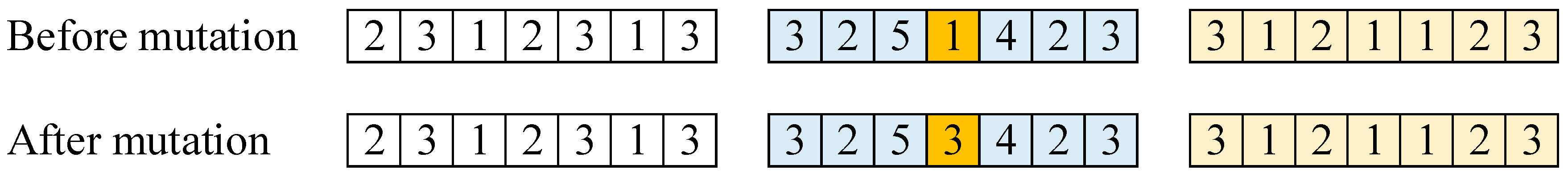
A one-point mutation operator was used in this study as shown in Figure 4. If the mutation point belonged to SgSo, the offspring generated by the mutation may be illegal coding, which should be repaired.

Step 5. Termination. When the number of iterations reaches the maximum, the best individual will be chosen as the result of the algorithm.

3.2. Sectional Encoding Discrete Particle Swarm Optimization

Step 1. Initializing parameters. The main content of it is setting the parameters in SE-DPSO, which include the number of the swarm (NS), the learning factor 1 (LF₁), the learning factor 2 (LF₂), the dimension of a particle (DP), the maximum number of iterations (NC_P_max), the inertia weight (ω), the related basic data and so on. The encoded description method is present in part of the SE-DPSO of Table 1. The 2nd column shows the dimension number of SgSo of a particle (P_r), and the column ‘dimension code (dc)’, the column ‘SgOm’ and the column ‘SgAt’ show the dimension codes of SgSo, SgOm, SgAt of a P_r respectively, which will be discussed later.

Step 2. Initializing swarm. A group of an initial swarm was created in this step. The initial position (p) and initial velocity (v) of a particle were generated by:

$$p_{\alpha \beta }^0=rand(0,1)$$

(28)

$$v_{\alpha \beta }^0=rand(0,1).$$

(29)

Here, α, β are the index of a particle and the index of a dimension in the particle.

Step 3. Particle encoding. Considering the discreteness of the dimension codes of a particle in this model, the smallest position value (SPV) rule and a discrete interval (DI) rule were applied to transfer the position of a particle to a set of dimension codes. The representations of the codes in SE-DPSO were the same as the codes in SE-GA. Two sub-steps for encoding a particle are as follows:

Applying SPV and DI rule. The SPV rule was used to transform the continuous codes in PSO to discrete codes that are applicable to all types of scheduling problems [15], so as the DI rule. The SPV rule was applied in SgSo while the DI rule was applied in the SgOm and SgAt of a particle.

Define the sequence of operations, operation-machine and AGV-task relationship. An example with two jobs, three machines, and six available AGVs is shown in

Table 2. Encoding of an example particle.

SgSo	Particle example	0.21	0.32	0.43	0.18	0.66	0.89
	Applying SPV rule	2	3	4	1	5	6
	Job codes	1	1	2	1	2	2
	Corresponding operations in each job	O1(1)	O1(2)	O2(1)	O1(3)	O2(2)	O2(3)
SgOm		0.1	0.3	0.5	0.7	0.3	0.7
	Corresponding machines	M1, M2, M3	M2, M3	M2	M1, M3	M2, M3	M1, M2
	Applying DI rule (Index of machines)	1	2	2	3	2	2
	Corresponding operations in each job	O1(1)	O1(2)	O1(3)	O2(1)	O2(2)	O2(3)
SgAt		0.93	0.21	0.49	0.37	0.86	0.18
	Applying DI rule (Index of AGVs)	6	2	3	3	6	2
	Corresponding operations in each job	O1(1)	O1(2)	O1(3)	O2(1)	O2(2)	O2(3)

for the explanation; both of the jobs include three operations. The assumed position of a particle for this example is shown in the 1st, 6th and 8th rows of Table 2. The definition method of the dimension codes of SgSo, SgOm, SgAt in a particle will be explained as follows respectively.

As shown in the 1st and 2nd rows of Table 2, the continuous codes of SgSo in the particle are (0.21, 0.32, 0.43, 0.18, 0.66, 0.89). According to the SPV rule, the corresponding discrete codes should be (2, 3, 4, 1, 5, 6). In descending order, 0.18 is the smallest value and its discrete code should be 1; 0.89 is the largest value and its discrete code should be 6 and so on. The 3rd row of Table 2 shows the job codes of SgSo in the particle; the smallest three numbers of the discrete codes in the 2nd row of Table 2 are assigned to the first job, so the job code should be 1. The largest three numbers are assigned to the second job, so the job code should be 2.

As shown in the 5th and 7th rows of Table 2, the position of SgOm in the particle is SgOm_P = (0.1, 0.3, 0.7, 0.2, 0.3, 0.7). According to the DI rule, the corresponding discrete codes should be SgOm_C = (1, 2, 3, 2, 2, 2). As shown in the 6th and 8th rows of Table 2, O₁(1) can be executed by M₁, M₂ and M₃. As a result, if SgOm_P(1) is between 0 and 0.33, then SgOm_C(1) should be 1; if SgOm_P(1) is between 0.34 and 0.66, then SgOm_C(1) should be 2 and so on. In the example, SgOm_P(1) is 0.1, which is between 0 and 0.33, so SgOm_C(1) should be 1. O₁(2) can be executed by M₂ and M₃. As a result, if SgOm_P(2) is between 0 and 0.50, then SgOm_C(2) should be 2, otherwise, SgOm_C(2) should be 3. In the example, SgOm_P(2) is 0.3, which is between 0 and 0.50, so SgOm_C(2) should be 2. O₁(3) can only be executed by M₂, so SgOm_C(3) should be 2.

As shown in the 9th and 10th rows of Table 2, the position of SgAt in the particle is (0.93, 0.21, 0.49, 0.37, 0.86, 0.18), according to the DI rule, the corresponding discrete codes are (6 2 3 3 6 2). Here, the number of available AGVs is six and the value 0.93 is between 5/6 and 6/6. Thus, the corresponding code should be 6; the value 0.21 is between 1/6 and 2/6, hence the corresponding code should be 2, and so on.

Step 4. Fitness evaluation. Each particle is evaluated by the makespan, total energy consumption and number of AGVs by Equations (1) to (17). In addition, the total fitness values will be calculated based on Equations (20) to (22).

Step 5. New swarm. The position and velocity of the particles were updated to generate a new swarm. Step 3, step 4 and step 5 were repeated up until the termination criterion.

The velocity of each particle was updated by:

$$v_{\alpha \beta }^{t+1}=\omega v_{\alpha \beta }^t+c_1{r}_1(p_{\alpha \beta }^{best}-p_{\alpha \beta }^t)+c_2{r}_2(g_{\beta }^{best}-p_{\alpha \beta }^t).$$

(30)

Here, c₁ is self-confidence and c₂ is swarm confidence. ω is the inertia weight, which is varying with a random method as shown in Equation (31).

$$\{\begin{array}{l}\omega =\mu +\sigma *N(0,1)\\ \mu ={\omega }_{min}+({\omega }_{max}-{\omega }_{min})*rand(0,1)\end{array}.$$

(31)

The position of the particle was updated by:

$$p_{\alpha \beta }^{t+1}=p_{\alpha \beta }^t+v_{\alpha \beta }^{t+1}.$$

(32)

Step 6. Termination. The iteration was terminated when the number of iterations reached its maximum, then the g^best was returned as the best solution.

4. Simulation Experiments and Discussion

4.1. Initial Data

To demonstrate the effectiveness of the proposed model, a numerical experiment was used in this paper. This experiment included eight jobs (J₁, ..., J₈) with 10 machines (M₁, …, M₁₀), and there were three to five operations in each job. In the experiment, up to six AGVs were available.

Table 3. Basic information about the relationship between operations and machines.

Job(Ji)	Mk/ ot(i,j)/ ec(i,j)/ wecu(k)
	Oi(1)	Oi(2)	Oi(3)	Oi(4)	Oi(5)
J1	M1/28/3.22/0.012 M4/25/2.91/0.012 M6/31/3.84/0.017	M2/21/3.82/0.015 M8/23/3.15/0.014	M5/22/2.67/0.011 M7/25/3.08/0.016 M10/27/2.72/0.021
J2	M3/12/2.15/0.020 M9/16/2.23/0.019	M2/24/2.53/0.015	M1/11/1.79/0.012 M8/15/1.93/0.014	M10/16/2.37/0.021	M5/18/2.44/0.011 M7/13/2.21/0.016
J3	M9/17/3.22/0.019	M2/18/2.78/0.015 M5/23/3.62/0.011 M7/21/2.50/0.016	M4/19/3.14/0.012 M8/15/2.93/0.014	M1/13/2.34/0.012 M6/16/2.45/0.017
J4	M2/22/3.25/0.015 M8/27/3.23/0.014	M1/19/3.33/0.012 M5/21/3.32/0.011	M3/23/3.67/0.020 M10/21/3.52/0.021	M6/28/4.13/0.017 M7/33/4.21/0.016
J5	M5/31/3.67/0.011 M10/27/3.55/0.021	M3/19/2.21/0.020 M4/24/2.32/0.012 M8/22/2.24/0.014	M1/14/2.54/0.012 M2/13/2.56/0.015 M9/16/2.63/0.019
J6	M4/25/3.11/0.012 M7/27/3.23/0.016	M3/30/4.11/0.020	M1/21/3.76/0.012 M5/18/3.68/0.011	M2/12/1.97/0.015 M9/15/1.91/0.019	M10/27/3.41/0.021
J7	M3/15/2.23/0.020 M6/19/2.27/0.017	M4/30/3.95/0.012 M7/33/3.87/0.016	M1/16/2.08/0.012 M8/17/2.11/0.014
J8	M5/23/3.54/0.011 M10/21/3.42/0.021	M3/25/3.73/0.020 M6/22/3.82/0.017	M2/27/4.21/0.015 M4/32/4.33/0.012

shows the associated data between the operations and machines.

Table 4. AGV traveling time among H points and machines.

Time(min)	H	M1	M2	M3	M4	M5	M6	M7	M8	M9	M10
H	0	7	11	16	12	10	20	8	19	18	23
M1	7	0	6	16	21	14	6	7	13	16	20
M2	11	6	0	21	9	7	11	18	23	15	22
M3	16	16	21	0	14	6	7	10	8	14	11
M4	12	21	9	14	0	11	17	13	22	5	19
M5	10	14	7	6	11	0	7	26	19	18	11
M6	20	6	11	7	17	7	0	4	13	17	18
M7	8	7	18	10	13	26	4	0	15	20	24
M8	19	13	23	8	22	19	13	15	0	13	19
M9	18	16	15	14	5	18	17	20	13	0	18
M10	23	20	22	11	19	11	18	24	19	18	0

shows the AGV travel time among H points and the machines.

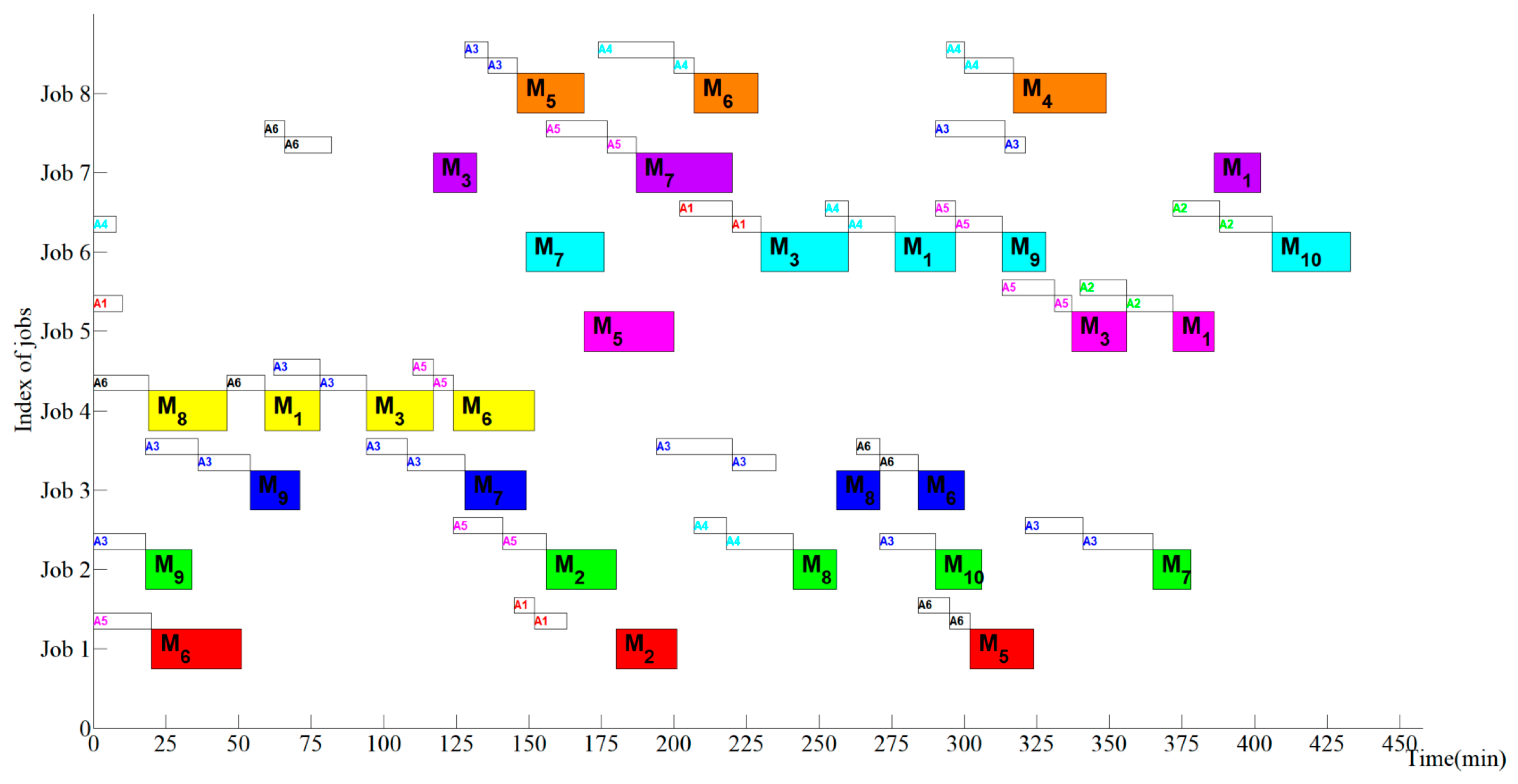
According to the data in Table 3 and Equation (17), the value of max(ese) in Equation (21) was calculated by:

$$max(ese)={\displaystyle \sum _{i=1}^n{\displaystyle \sum _{j=1}^{m_i}max(es(i,j)}}).$$

(33)

Therefore, the value of max(ese) is 94.25. Figure 5 shows the Gantt chart before optimization by a random execution sequence and traveling sequence with six AGVs for the experiment, where Ai represents AGV i. The nearest bars on the left side of each operation indicate the time that the AGV transports the job from the previous operation to that operation, where the first bar and second bar indicate the running time of the AGV with no-load and load respectively. The values of fitness, number of AGVs, makespan, and energy consumption are 6, 420.67, 433 and 134.51 respectively. It is just an available random scheme for this experiment and all of the six AGVs were applied; it is difficult to be chosen as a high-quality solution. To optimize the solution for this experiment in FMS, the EAs proposed in this paper were applied and verified in the next section.

4.2. Parameters of the Algorithms Setting

The selection of parameters has a significant impact on the performance of the algorithms. To get the best settings and parameters of the H-SE-GA-DPSO that can provide the best performance within a reasonable computation time, a parameter test experiment, based on an orthogonal design method which is a low cost and effective parameter test method, was performed with the data as shown in Section 4.1. In the experiment, four levels and eight factors, as shown in

Table 5. Factors and their levels.

Levels	Factors
	PS	CR	MR	c1	c2	wmin	wmax	σ
1	100	0.2	0.05	0.01	0.3	0.01	0.3	0.2
2	150	0.4	0.08	0.05	0.5	0.05	0.5	0.4
3	200	0.6	0.1	0.1	0.7	0.1	0.7	0.6
4	300	0.8	0.2	0.2	0.9	0.2	0.9	0.8

, were applied. The experimental results are shown in

Table 6. Experimental results of orthogonal test of the parameters of hybrid sectional encoding genetic algorithm and discrete particle swarm optimization (H-SE-GA-DPSO).

Index	PS	CR	MR	c1	c2	wmin	wmax	σ	Fitnesses	Time
1	100	0.2	0.05	0.01	0.3	0.01	0.3	0.2	274.93	84.67
2	100	0.4	0.08	0.05	0.5	0.05	0.5	0.4	273.90	85.12
3	100	0.6	0.1	0.1	0.7	0.1	0.7	0.6	271.24	85.18
4	100	0.8	0.2	0.2	0.9	0.2	0.9	0.8	299.52	85.37
5	150	0.2	0.05	0.05	0.5	0.1	0.7	0.8	276.37	120.07
6	150	0.4	0.08	0.01	0.3	0.2	0.9	0.6	272.72	117.92
7	150	0.6	0.1	0.2	0.9	0.01	0.3	0.4	273.69	119.26
8	150	0.8	0.2	0.1	0.7	0.05	0.5	0.2	272.06	124.39
9	200	0.2	0.08	0.1	0.9	0.01	0.5	0.6	272.02	168.32
10	200	0.4	0.05	0.2	0.7	0.05	0.3	0.8	273.08	168.21
11	200	0.6	0.2	0.01	0.5	0.1	0.9	0.2	268.01	169.05
12	200	0.8	0.1	0.05	0.3	0.2	0.7	0.4	271.51	168.23
13	300	0.2	0.08	0.2	0.7	0.1	0.9	0.4	275.29	247.08
14	300	0.4	0.05	0.1	0.9	0.2	0.7	0.2	263.67	249.13
15	300	0.6	0.2	0.05	0.3	0.01	0.5	0.8	270.88	251.51
16	300	0.8	0.1	0.01	0.5	0.05	0.3	0.6	269.30	249.74
17	100	0.2	0.2	0.01	0.9	0.05	0.7	0.4	276.15	82.77
18	100	0.4	0.1	0.05	0.7	0.01	0.9	0.2	275.87	96.53
19	100	0.6	0.08	0.1	0.5	0.2	0.3	0.8	270.46	92.71
20	100	0.8	0.05	0.2	0.3	0.1	0.5	0.6	272.73	93.06
21	150	0.2	0.2	0.05	0.7	0.2	0.3	0.6	267.76	131.14
22	150	0.4	0.1	0.01	0.9	0.1	0.5	0.8	285.97	125.89
23	150	0.6	0.08	0.2	0.3	0.05	0.7	0.2	277.42	146.37
24	150	0.8	0.05	0.1	0.5	0.01	0.9	0.4	271.09	151.61
25	200	0.2	0.1	0.1	0.3	0.05	0.9	0.8	276.93	174.32
26	200	0.4	0.2	0.2	0.5	0.01	0.7	0.6	273.46	169.82
27	200	0.6	0.05	0.01	0.7	0.2	0.5	0.4	272.31	168.94
28	200	0.8	0.08	0.05	0.9	0.1	0.3	0.2	277.92	170.27
29	300	0.2	0.1	0.2	0.5	0.2	0.5	0.2	280.28	259.37
30	300	0.4	0.2	0.1	0.3	0.1	0.3	0.4	272.58	246.45
31	300	0.6	0.05	0.05	0.9	0.05	0.9	0.6	274.05	247.34
32	300	0.8	0.08	0.01	0.7	0.01	0.7	0.8	277.16	252.66
33	100	0.2	0.08	0.01	0.9	0.01	0.5	0.6	272.94	95.31

. Here, each group of data was run 20 times with 500 iterations and the average value was taken as the result.

As shown in Table 6, it can be observed that the data in group 21 were the best configuration of parameters, which provide the optimal solution within a reasonable computation time. According to the data in Table 5, it can be observed that a larger population leads to a longer computation time. Besides, compared with other groups of data, the values of CR and w_max of group 21 were smaller while the values of MR and w_min were larger; they and the values of the other parameters affect the performance of the algorithm together. Therefore, to obtain optimal solutions and to ensure the effective comparison of the algorithms within a reasonable computation time, the parameters setting of each algorithm are shown in

Table 7. Parameters setting of each algorithm.

Algorithms	Parameters
SE-GA	PS = 150, CR = 0.2, MR = 0.2
SE-DPSO	PS = 150, c1 = 0.05, c2 = 0.7, wmin = 0.2, wmax = 0.3, σ = 0.6
H-SE-GA-DPSO	PS = 150, CR = 0.2, MR = 0.2, c1 = 0.05, c2 = 0.7, wmin = 0.2, wmax = 0.3, σ = 0.6
H-GA-PSO	PS = 150, CR = 0.2, MR = 0.2, c1 = 0.05, c2 = 0.7, wmin = 0.2, wmax = 0.3, σ = 0.6
TSA	Based on the related literature [9]

.

4.3. Experiment Results and Discussion

The parameters for the hardware and software platform are list as follows: Windows 10, IntelIntel®Core™ i7-4700MQ CPU, 2.40 GHz, 8 GB of RAM and the MATLAB 2016a (MathWorks, Natick City, U.S.).

To verify the effectiveness of the algorithms proposed in this paper and the advantages of H-SE-GA-DPSO over other algorithms, we performed a comparative experiment among the algorithms. All the algorithms were run 20 times with 500 iterations by considering the complexity of the problem.

In this experiment, the value of DT was 400. ψ₁ and ψ₂ were calculated based on Equations (21) and (22) respectively. The values of φ₁, φ₂ and φ₃ were presumed to be 0.5, 0.2 and 0.3 respectively. In

Table 8. The best optimization results of the five algorithms.

Algorithms	Average Values of Fitness	Average Values of Makespan	Average Values of Energy Consumption	Average Numbers of AGVs	Values of Mean Computational Time
SE-GA	286.76	241.40	109.05	4.90	82.33
SE-DPSO	311.43	263.45	111.87	5.65	96.16
H-SE-GA-DPSO	267.76	211.85	104.95	4.85	131.14
H-GA-PSO	310.13	253.00	111.19	5.95	137.86
TSA	272.45	216.95	106.60	4.90	148.69

, the fitness values were calculated based on Equation (20).

The best optimization results of the five algorithms are shown in Table 8, and the results are the average values after the algorithms being run 20 times. Compared with the result before optimization, as shown in Figure 5, the algorithms were proven to be effective in optimizing FMS scheduling with AGVs, and the number of AGVs decreases after optimization with SE-GA, H-SE-GA-DPSO and TSA. Compared with SE-GA and SE-DPSO, H-SE-GA-DPSO can get a better solution on all the three objectives even though they are all trying to solve the problem proposed on the three dimensions. Therefore, the performance of the hybrid algorithm was improved. Compared with H-GA-PSO and TSA, H-SE-GA-DPSO also can get a better comprehensive solution, although TSA can get a good result, the longer computational time discounted it; besides, compared with H-SE-GA-DPSO, the energy consumption of the result obtained by TSA was higher for ignoring the optimization of machine selection. Therefore, H-SE-GA-DPSO was verified to be superior to the other algorithms.

The 20 groups of data corresponding to the results of 20 runs of each algorithm are shown in

Table 9. The 20 groups of data corresponding to the results of 20 runs of each algorithm.

Group Numbers	SE-GA		SE-DPSO		H-SE-GA-DPSO		H-GA-PSO		TSA
	Fitness Values	NA	Fitness Values	NA	Fitness Values	NA	Fitness Values	NA	Fitness Values	NA
1	283.97	5	302.61	6	267.02	5	311.34	6	268.14	4
2	288.22	5	303.77	6	272.47	5	303.71	6	268.05	4
3	280.47	5	297.10	6	264.84	5	319.92	6	257.24	5
4	290.13	5	314.55	6	272.16	5	298.77	6	274.32	6
5	286.47	5	304.89	6	262.00	5	308.00	6	266.79	5
6	286.60	4	318.13	5	270.36	5	297.91	6	272.21	5
7	288.38	5	305.45	5	271.25	5	318.64	6	259.46	5
8	297.83	6	317.55	6	260.91	5	312.78	6	276.08	5
9	303.52	5	325.18	6	271.62	5	311.86	6	262.57	5
10	279.32	5	316.09	5	264.26	4	309.95	6	270.11	4
11	283.85	5	299.63	6	274.43	5	303.21	6	276.49	4
12	277.01	5	322.33	6	261.51	4	309.85	6	275.45	6
13	283.42	4	291.04	6	269.45	5	310.76	6	267.69	4
14	290.57	6	316.45	6	258.78	5	315.64	6	281.90	5
15	279.99	4	309.10	6	266.22	5	315.64	6	281.97	6
16	290.95	6	342.85	4	270.40	5	315.07	6	281.75	5
17	280.45	5	307.36	5	276.77	4	316.68	6	268.66	4
18	289.96	5	314.90	5	262.12	5	310.88	5	266.19	5
19	277.39	4	313.54	6	268.98	5	302.03	6	296.97	6
20	296.76	4	306.07	6	269.60	5	309.90	6	277.03	5

. It can be observed that the optimal number of AGVs optimized with H-SE-GA-DPSO in this experiment can be four or five. Besides, according to the results of each algorithm in Table 9, compared with the other algorithms, the results of H-SE-GA-DPSO had a smaller fluctuation range. As a result, the H-SE-GA-DPSO is more stable for optimizing fitness and minimizing the number of AGVs than the other algorithms.

As shown in

Table 10. The experiments with different numbers of available AGVs using H-SE-GA-DPSO.

Data items	Numbers of Available AGVs
	6	7	8	9	10
Average values of fitness	267.76	268.11	270.20	273.45	276.03
Average numbers of AGV	4.85	4.95	5.15	5.20	5.40
Number of AGVs	4(3), 5(17)	4(2), 5(17), 6(1)	4(1), 5(15), 6(4)	5(16), 6(4)	4(2), 5(10), 6(6), 7(2)

, the experiments based on the data in Section 4.1 with different numbers of available AGVs were performed and the results are presented in the table. Here, each experiment was run 20 times using the H-SE-GA-DPSO. In Table 10, the numbers in parentheses indicate the frequencies that those numbers themselves appeared in the corresponding experiment. According to the results, four and five were further proven to be the optimal numbers of AGVs to meet the needs of the jobs in Section 4.1. As the number of available AGVs increases, six and seven were also selected as the optimal numbers of AGVs, which led to the increase of the values of fitness. Therefore, the results of H-SE-GA-DPSO can be influenced by the number of available AGVs to a certain extent. However, the H-SE-GA-DPSO was also proven to be stable and effective over a wide range.

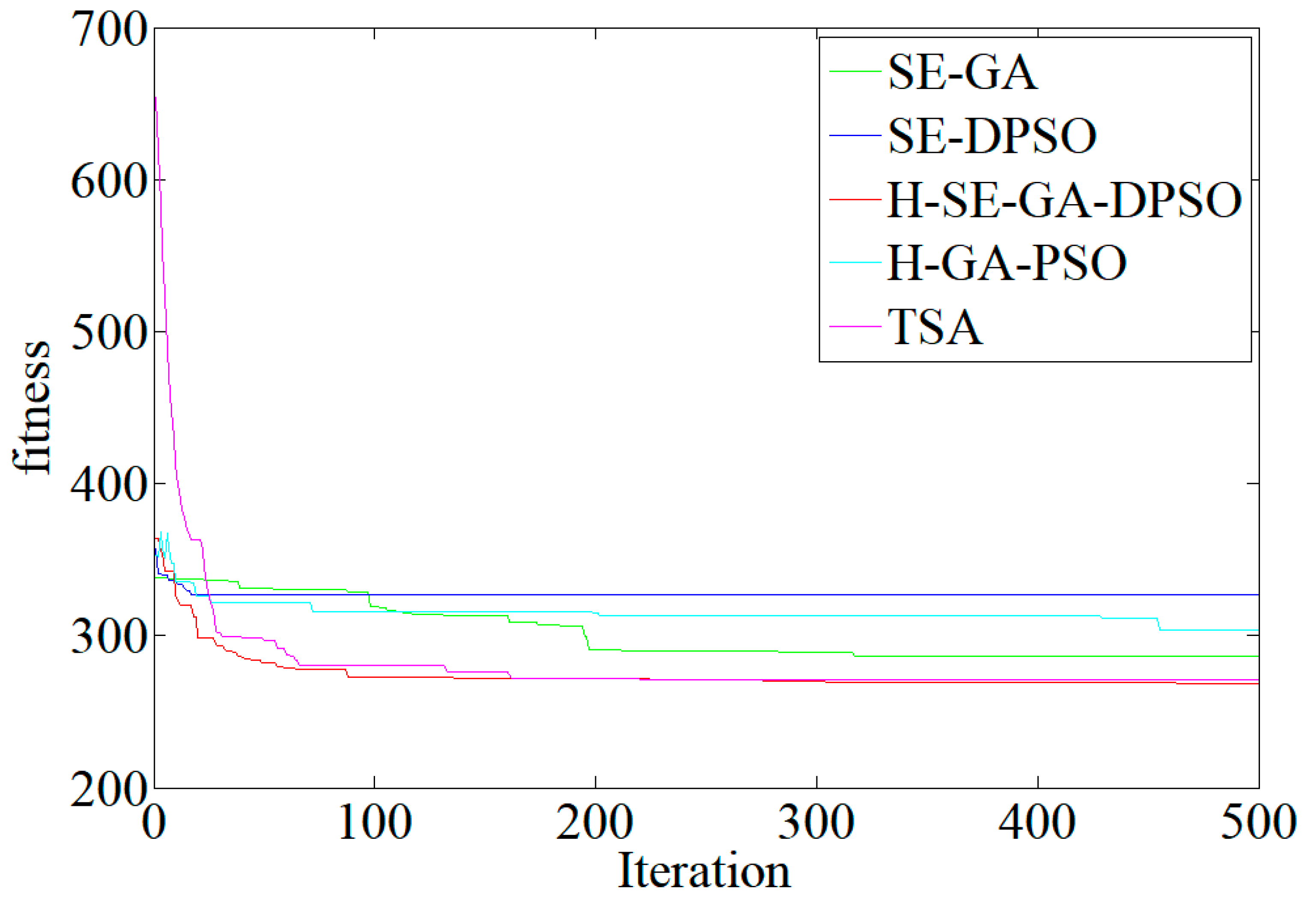
Figure 6 shows the performance of SE-GA, SE-DPSO, H-SE-GA-DPSO, H-GA-PSO and TSA in the experiment above with six available AGVs. SE-DPSO was easy to fall into local convergence in this experiment and H-GA-PSO just took the sequence of operations into account; the convergence of the results was not satisfactory. Although SE-GA had a good convergence effect, its convergence rate was slower than that of H-SE-GA-DPSO and TSA. Compared with the other algorithms, H-SE-GA-DPSO and TSA had a good convergence rate and result, and the result of H-SE-GA-DPSO was slightly better than that of TSA, which can be attributed to the consideration of machine selection in H-SE-GA-DPSO.

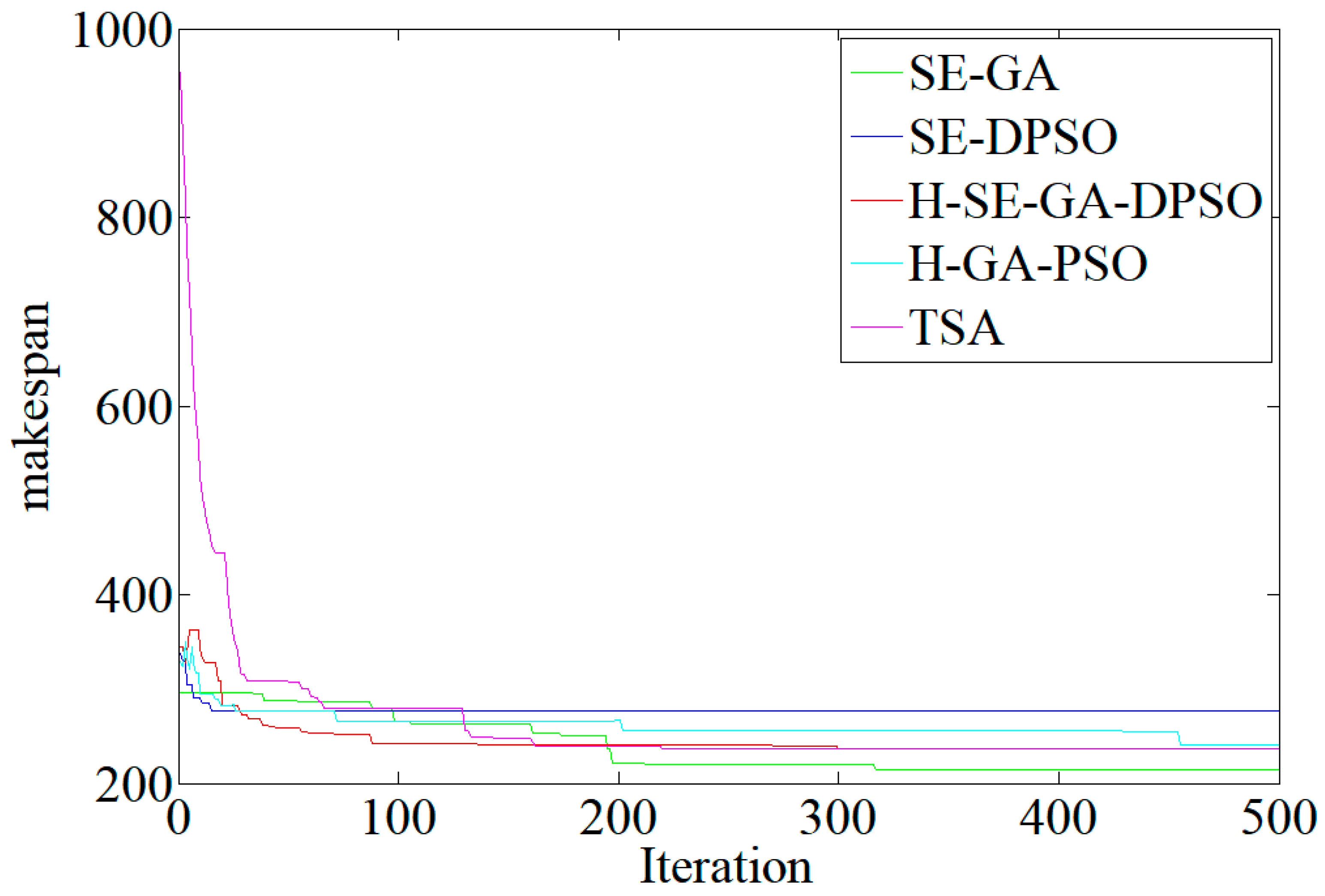
The evolutionary curves of the makespan of the best fitness with six available AGVs are shown in Figure 7. The convergence trends of them are roughly the same as the curves in Figure 6; H-SE-GA-DPSO and TSA had a better optimization effect on the makespan.

Figure 8 shows the evolutionary curves of energy consumption of the best fitness with six available AGVs. It can be easily observed that the values of energy consumption converge quickly and fluctuate within a certain range. In this aspect, the convergence result of H-SE-GA-DPSO was obviously better than the TSA. Therefore, it is significant to consider machine selection on AGVs scheduling in FMS.

Figure 9 shows the evolutionary curves of a number of AGVs of the best fitness with six available AGVs. The evolutionary process of them was relatively simple. The number of AGVs was minimized in the results obtained by H-SE-GA-DPSO and TSA. The numbers of AGVs obtained by other algorithms was influenced by the initial population to some extent.

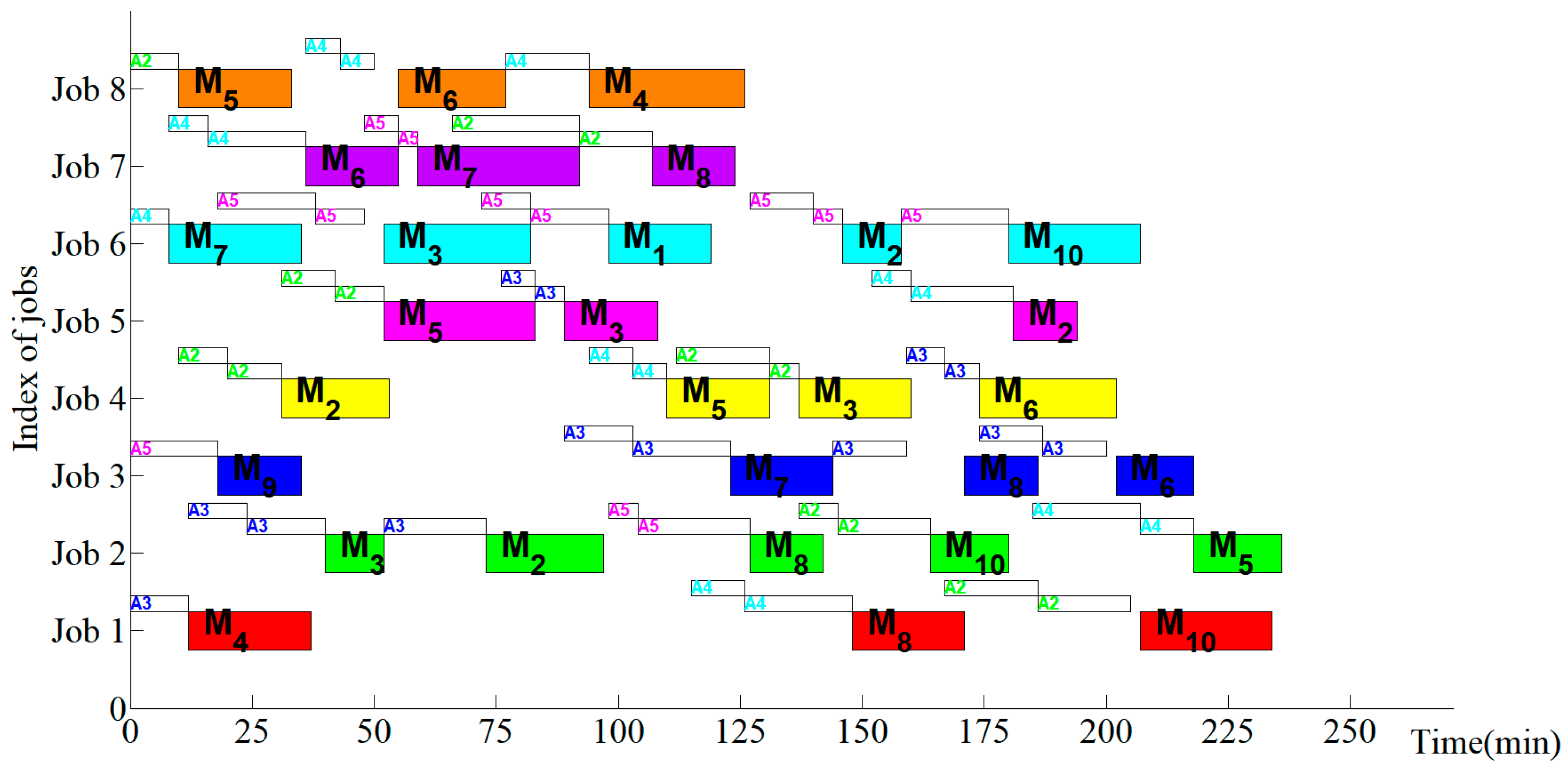
Figure 10 shows the optimization sequence using only four AGVs, which was obtained by H-SE-GA-DPSO. Compared with the sequence in Figure 5, all jobs were completed in less time, although the number of AGVs was less. In Figure 6 and Figure 8, the fitness and energy consumption were also less than that of the sequence in Figure 5. Overall, the application of H-SE-GA-DPSO to solve a multi-objective and multi-dimensional scheduling problem is concluded to be an effective method.

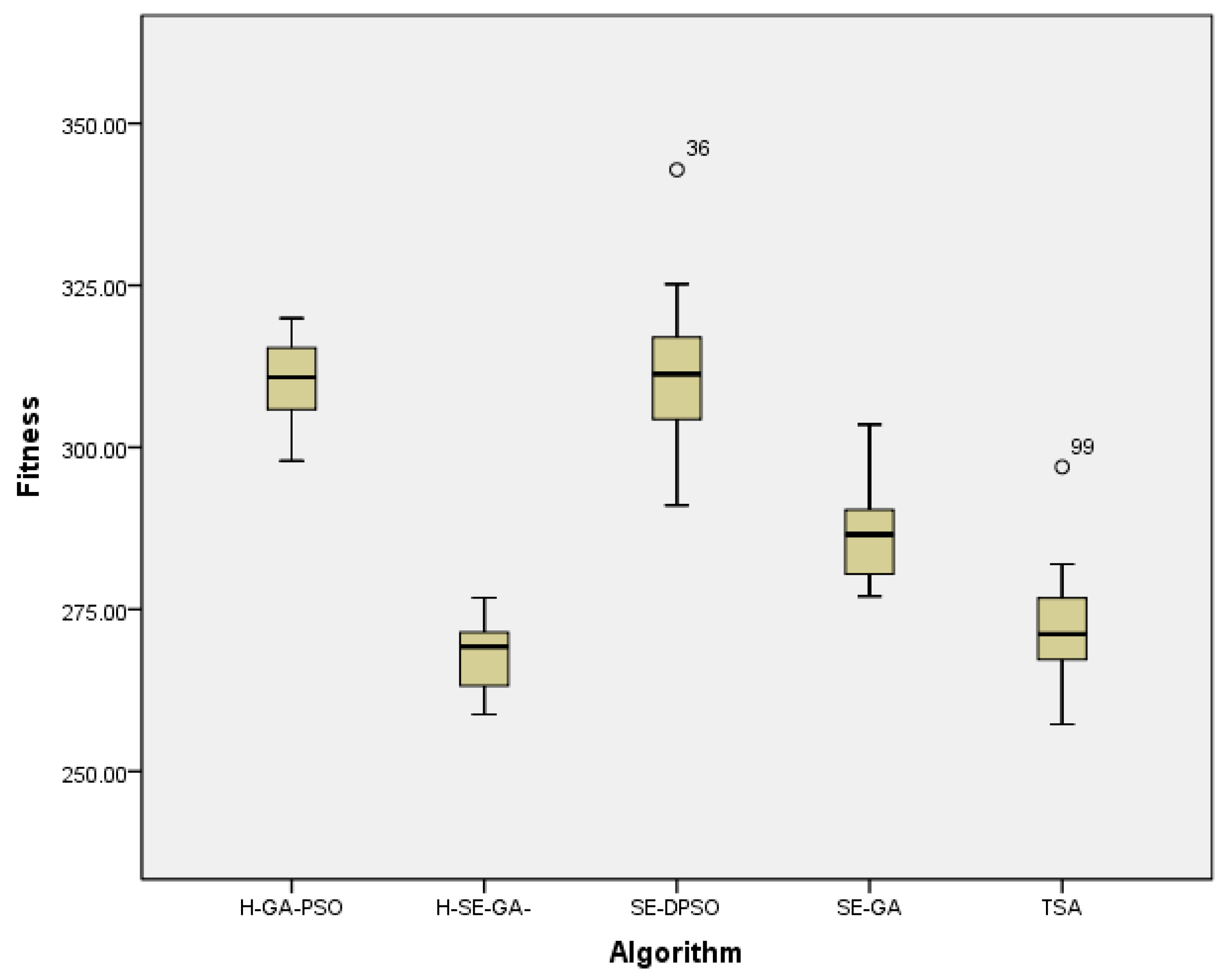
To further verify the conclusion, a significance test of the results of the algorithms is provided. According to the data of the fitness values in Table 9, we can get the data as shown in

Table 11. The results of the normal distribution test using the Shapiro-Wilk method.

Algorithms	SE-GA	SE-DPSO	H-SE-GA-DPSO	H-GA-PSO	TSA
Significance (p-value)	0.319	0.388	0.599	0.335	0.365

using the Shapiro-Wilk test and the corresponding box-plot is shown in Figure 11. In this test, the significance level was α=0.05 and all of the p-values were larger than α. Therefore, the data obtained by the five algorithms conform to a normal distribution. To analyze statistically significant differences in the data, The tukey HSD method was applied in this paper.

Table 12. The results of the test of homogeneity of variances.

Levene Statistic	degree of Freedom 1 (df1)	degree of Freedom 2 (df2)	p-Value
2.743	4	95	0.033

shows the results of the test of homogeneity of variances. Here, the significance level was also 0.05, so the variances don’t satisfy the condition of homogeneity. The data of robust tests of equality of means obtained by the methods of Welch and Brown-Forsythe show that the p-values were 0.00, which is smaller than 0.05. Therefore, statistically significant differences among the fitness values were obtained with different algorithms in this paper. In summary, the advantages of H-SE-GA-DPSO over other algorithms were further verified.

5. Conclusions and Future Work

Aimed at the AGV optimization scheduling problem in an FMS environment, this research developed a multi-objective and multi-dimensional optimization scheduling mathematical model while considering energy consumption and multi-function of the machines. In this model, the multi-objective was to minimize the makespan and energy consumption of machines and the number of AGVs. The multi-dimensional objective was to simultaneously optimize the sequence of operations of related jobs, the matching relation between transfer tasks and AGVs (AGV-task) and the matching relation between operations and machines (operation-machine) for the multi-objective.

To meet the needs of the above model, three evolutionary algorithms (SE-GA, SE-DPSO and H-SE-GA-DPSO) have been developed to realize multi-objective and multi-dimensional optimization scheduling, which have been proven to be effective. According to the results of the comparison, the superiority of H-SE-GA-DPSO over the other algorithms was proven. Overall, H-SE-GA-DPSO is a good optimization method in multi-objective and multi-dimensional scheduling of FMS with AGVs, and it can also be applied to more situations with the development of intelligent manufacturing and green manufacturing.

In the future, it will be interesting to investigate the following issues:

The model proposed in this paper should be stretched from a workshop level to an enterprise level and more factors should be taken into account for deeper optimization. H-SE-GA-DPSO should be applied in a distributed computing environment to meet more complex computing needs.

References

- Guo, Q.; Zhang, M. A novel approach for multi-agent-based Intelligent Manufacturing System. Inf. Sci. 2009, 179, 3079–3090. [Google Scholar] [CrossRef]
- Kang, H.S.; Ju, Y.L.; Choi, S.S.; Kim, H.; Park, J.; Son, J.; Kim, B.; Noh, S. Smart manufacturing: Past research, present findings, and future directions. Int. J. Precis. Eng. Manuf. Green Technol. 2016, 3, 111–128. [Google Scholar] [CrossRef]
- Huang, S.; Guo, Y.; Zha, S.; Wang, F.; Fang, W. A Real-time Location System Based on RFID and UWB for Digital Manufacturing Workshop. Procedia CIRP 2017, 63, 132–137. [Google Scholar] [CrossRef]
- Confessore, G.; Fabiano, M.; Liotta, G. A network flow based heuristic approach for optimising AGV movements. J. Intell. Manuf. 2013, 24, 405–419. [Google Scholar] [CrossRef]
- Srivastava, S.C.; Choudhary, A.K.; Kumar, S.; Tiwari, M.K. Development of an intelligent agent-based AGV controller for a flexible manufacturing system. Int. J. Adv. Manuf. Technol. 2008, 36, 780. [Google Scholar] [CrossRef]
- Singh, N.; Sarngadharan, P.V.; Pal, P.K. AGV scheduling for automated material distribution: A case study. J. Intell. Manuf. 2011, 22, 219–228. [Google Scholar] [CrossRef]
- Ramana, B.; Reddy, S.S.; Ramprasad, B. Quantitative Analysis of AGV System in FMS Cell Layout. Def. Sci. J. 2013, 47, 75–81. [Google Scholar] [CrossRef]
- Murata, T. Makespan Minimization of Machines and Automated Guided Vehicles Schedule Using Binary Particle Swarm Optimization. In Proceedings of the Proceedings of the International Multiconference of Engineers and Computer Scientists, Hong Kong, China, 17–19 March 2010; pp. 268–272. [Google Scholar]
- Zheng, Y.; Xiao, Y.; Seo, Y. A tabu search algorithm for simultaneous machine/AGV scheduling problem. Int. J. Prod. Res. 2014, 52, 5748–5763. [Google Scholar] [CrossRef]
- Deroussi, L.; Gourgand, M.; Tchernev, N. A simple metaheuristic approach to the simultaneous scheduling of machines and automated guided vehicles. Int. J. Prod. Res. 2008, 46, 2143–2164. [Google Scholar] [CrossRef]
- Lacomme, P.; Larabi, M.; Tchernev, N. Job-shop based framework for simultaneous scheduling of machines and automated guided vehicles. Int. J. Prod. Econ. 2013, 143, 24–34. [Google Scholar] [CrossRef]
- Baruwa, O.T.; Piera, M.A. A coloured Petri net-based hybrid heuristic search approach to simultaneous scheduling of machines and automated guided vehicles. Int. J. Prod. Res. 2016, 54, 1–20. [Google Scholar] [CrossRef]
- Udhayakumar, P.; Kumanan, S. Task scheduling of AGV in FMS using non-traditional optimization techniques. Int. J. Simul. Model. 2010, 9, 28–39. [Google Scholar] [CrossRef]
- Pan, X.Y.; Wu, J.; Zhang, Q.W.; Lai, D.; Xie, H.; Zhang, Z. A Case Study of AGV Scheduling for Production Material Handling. Appl. Mechan. Mater. 2013, 411–414, 2351–2354. [Google Scholar] [CrossRef]
- Mousavi, M.; Yap, H.J.; Musa, S.N.; Tahriri, F.; Dawal, S.Z.M. Multi-objective AGV scheduling in an FMS using a hybrid of genetic algorithm and particle swarm optimization. PLoS ONE 2017, 12, e0169817. [Google Scholar] [CrossRef] [PubMed]
- Mousavi, M.; Yap, H.J.; Musa, S.N. A fuzzy hybrid GA-PSO algorithm for multi-objective AGV scheduling in FMS. Int. J. Simul. Model. 2017, 16, 58–71. [Google Scholar] [CrossRef]
- Cai, Q.; Tang, D.; Zheng, K.; Zhu, H.; Wu, X.; Lu, X. Multi-AGV scheduling optimization based on: Neuro-endocrine coordination mechanism. Int. J. Smart Sens. Intell. Syst. 2013, 7, 1613–1630. [Google Scholar] [CrossRef]
- Novas, J.M.; Henning, G.P. Integrated scheduling of resource-constrained flexible manufacturing systems using constraint programming. Expert Syst. Appl. 2014, 41, 2286–2299. [Google Scholar] [CrossRef]
- Mchaney, R. Modelling battery constraints in discrete event automated guided vehicle simulations. Int. J. Prod. Res. 2007, 33, 3023–3040. [Google Scholar] [CrossRef]
- Kabir, Q.S.; Suzuki, Y. Increasing manufacturing flexibility through battery management of automated guided vehicles. Comput. Ind. Eng. 2018, 117, 225–236. [Google Scholar] [CrossRef]
- Yan, R.; Jackson, L.M.; Dunnett, S.J. Automated guided vehicle mission reliability modelling using a combined fault tree and Petri net approach. Int. J. Adv. Manuf. Technol. 2017, 92, 1825–1837. [Google Scholar] [CrossRef]
- Tao, F.; Hu, Y.; Zhou, Z. Correlation-aware resource service composition and optimal-selection in manufacturing grid. Eur. J. Oper. Res. 2010, 201, 129–143. [Google Scholar] [CrossRef]
- Guo, S.; Du, B.; Peng, Z.; Huang, X.; Li, Y. Manufacturing resource combinatorial optimization for large complex equipment in group manufacturing: A cluster-based genetic algorithm. Mechatronics 2015, 31, 101–115. [Google Scholar] [CrossRef]
- Du, B.; Guo, S.; Huang, X.; Li, Y.; Guo, J. A Pareto supplier selection algorithm for minimum the life cycle cost of complex product system. Expert Syst. Appl. 2015, 42, 4253–4264. [Google Scholar] [CrossRef]
- Wang, L.; Guo, S.; Li, X.; Du, B.; Xu, W. Distributed manufacturing resource selection strategy in cloud manufacturing. Int. J. Adv. Manuf. Technol. 2018, 94, 3375–3388. [Google Scholar] [CrossRef]
- Udhayakumar, P.; Kumanan, S. Integrated scheduling of flexible manufacturing system using evolutionary algorithms. Int. J. Adv. Manuf. Technol. 2012, 61, 621–635. [Google Scholar] [CrossRef]
- Caridá, V.F.; Morandin, O.; Tuma CC, M. Approaches of fuzzy systems applied to an AGV dispatching system in a FMS. Int. J. Adv. Manuf. Technol. 2015, 79, 615–625. [Google Scholar] [CrossRef]
- Chang, H.C.; Liu, T.K. Optimisation of distributed manufacturing flexible job shop scheduling by using hybrid genetic algorithms. J. Intell. Manuf. 2017, 28, 1973–1986. [Google Scholar] [CrossRef]
- Rifai, A.P.; Nguyen, H.T.; Aoyama, H.; Dawal, S.Z.M.; Masruroh, N.A. Non-dominated sorting biogeography-based optimization for bi-objective reentrant flexible manufacturing system scheduling. Appl. Soft Comput. 2018. [Google Scholar] [CrossRef]
- Proth, J.M.; Sauer, N.; Xie, X. Optimization of the number of transportation devices in a flexible manufacturing system using event graphs. IEEE Trans. Ind. Electron. 2006, 44, 298–306. [Google Scholar] [CrossRef]
- Saidi-Mehrabad, M.; Dehnavi-Arani, S.; Evazabadian, F.; Mahmoodian, V. An Ant Colony Algorithm (ACA) for solving the new integrated model of job shop scheduling and conflict-free routing of AGVs. Comput. Ind. Eng. 2015, 86, 2–13. [Google Scholar] [CrossRef]
- Pjevcevic, D.; Nikolic, M.; Vidic, N.; Vukadinovic, K. Data envelopment analysis of AGV fleet sizing at a port container terminal. Int. J. Prod. Res. 2017, 55, 4021–4034. [Google Scholar] [CrossRef]
- Vivaldini, K.; Rocha, L.F.; Martarelli, N.J.; Becker, M.; Moreira, A.P. Integrated tasks assignment and routing for the estimation of the optimal number of AGVS. Int. J. Adv. Manuf. Technol. 2016, 82, 719–736. [Google Scholar] [CrossRef]
- Yan, H.E. Job scheduling model of machining system for green manufacturing. Chin. J. Mech. Eng. 2007, 43, 27–33. [Google Scholar]
- Govindan, K.; Diabat, A.; Shankar, K.M. Analyzing the drivers of green manufacturing with fuzzy approach. J. Clean. Prod. 2015, 96, 182–193. [Google Scholar] [CrossRef]
- Singh, A.; Philip, D.; Ramkumar, J.; Das, M. A simulation based approach to realize green factory from unit green manufacturing processes. J. Clean. Prod. 2018, 182, 67–81. [Google Scholar] [CrossRef]
- Liang, Y.; Lin, L.; Gen, M.; Chien, C. A hybrid evolutionary algorithm for fms optimization with AGV dispatching. Comput. Ind. Eng. 2012, 2, 1115–1128. [Google Scholar]
- Chen, R.M.; Shen, Y.M. Dynamic search control-based particle swarm optimization for project scheduling problems. Adv. Mech. Eng. 2016, 8, 1687814016641837. [Google Scholar] [CrossRef]
- Lu, H.; Zhou, R.; Fei, Z.; Shi, J. A multi-objective evolutionary algorithm based on Pareto prediction for automatic test task scheduling problems. Appl. Soft Comput. 2018. [Google Scholar] [CrossRef]
- Wang, Z.; Si, L.; Tan, C.; Liu, X. A Novel Approach for Shearer Cutting Load Identification through Integration of Improved Particle Swarm Optimization and Wavelet Neural Network. Adv. Mech. Eng. 2014, 2014, 521629. [Google Scholar] [CrossRef]
- Giagkiozis, I.; Fleming, P.J. Methods for multi-objective optimization: An analysis. Inf. Sci. 2015, 293, 338–350. [Google Scholar] [CrossRef] [Green Version]
- Han, D.; Yang, B.; Li, J.; Wang, J.; Sun, M.; Zhou, Q. A multi-agent-based system for two-stage scheduling problem of offshore project. Adv. Mech. Eng. 2017, 9, 1–17. [Google Scholar] [CrossRef]
- Kim, J.W.; Sang, W.K. New Encoding/Converting Methods of Binary GA/Real-Coded GA. IEICE Trans. Fundam. Electron. Commun. Comput. Sci. 2005, 88, 1554–1564. [Google Scholar] [CrossRef]
- Yamamoto, H.; Qudeiri, J.A.; Yamada, T.; Rizauddin, R. Production layout design system by GA with one by one encoding method. Artif. Life Robot. 2008, 13, 234–237. [Google Scholar] [CrossRef]
- Wang, H.F.; Hsu, H.W. A closed-loop logistic model with a spanning-tree based genetic algorithm. Comput. Oper. Res. 2010, 37, 376–389. [Google Scholar] [CrossRef]
- Zhang, Y.; Liu, M. An improved genetic algorithm encoded by adaptive degressive ary number. Soft Comput. 2018, 22, 6861–6875. [Google Scholar] [CrossRef]
- Wu, J.; Zhang, C.H.; Cui, N.X. PSO algorithm-based parameter optimization for HEV powertrain and its control strategy. Int. J. Automot. Technol. 2008, 9, 53–59. [Google Scholar] [CrossRef]
- Ishaque, K.; Salam, Z.; Amjad, M.; Mekhilef, S. An Improved Particle Swarm Optimization (PSO)-Based MPPT for PV With Reduced Steady-State Oscillation. IEEE Trans. Power Electron. 2012, 27, 3627–3638. [Google Scholar] [CrossRef]
- Tian, Y.; Liu, D.; Yuan, D.; Wang, K. A discrete PSO for two-stage assembly scheduling problem. Int. J. Adv. Manuf. Technol. 2013, 66, 481–499. [Google Scholar] [CrossRef]
- Shi, X.H.; Liang, Y.C.; Leeb, H.P.; Lu, C.; Wang, L.M. An improved GA and a novel PSO-GA-based hybrid algorithm. Inf. Process. Lett. 2005, 93, 255–261. [Google Scholar] [CrossRef]
- Li, J.; Yang, B.; Zhang, D.; Zhou, Q.; Li, L. Development of a multi-objective scheduling system for offshore projects based on hybrid non-dominated sorting genetic algorithm. Adv. Mech. Eng. 2015, 7, 1687814015573785. [Google Scholar] [CrossRef]
- Su, Y.; Chu, X.; Zhang, Z.; Chen, D. Process planning optimization on turning machine tool using a hybrid genetic algorithm with local search approach. Adv. Mech. Eng. 2015, 7, 1687814015581241. [Google Scholar] [CrossRef]
Figure 1.
Schematic diagram of multi-objective optimization scheduling problems in the model by considering multiple optimization dimensions.
Figure 2.
The main flowchart and methods of hybrid sectional encoding genetic algorithm and discrete particle swarm optimization (H-SE-GA-DPSO).
Figure 3.
Example of two-point crossover of chromosomes.
Figure 4.
An example of a hybrid mutation operator of the chromosome.
Figure 5.
Gantt chart of a random sequence of the experiment using six automated guided vehicles (AGVs) before optimization.
Figure 6.
Evolutionary curves of the best fitness using the five algorithms with six available AGVs.
Figure 7.
Evolutionary curves of the makespan of the best fitness using the five algorithms with six available AGVs.
Figure 8.
Evolutionary curves of energy consumption of the best fitness using the five algorithms with six available AGVs.
Figure 9.
Evolutionary curves of the number of AGVs of the best fitness using the five algorithms with six available AGVs.
Figure 10.
Gantt chart of the experiment after optimization by H-SE-GA-DPSO.
Figure 11.
The box-plot of fitness values obtained by the five algorithms.