Control Strategy of a Hybrid Energy Storage System to Smooth Photovoltaic Power Fluctuations Considering Photovoltaic Output Power Curtailment

Abstract

The power fluctuations of grid-connected photovoltaic (PV) systems have negative impacts on the power quality and stability of the utility grid. In this study, the combinations of a battery/supercapacitor hybrid energy storage system (HESS) and the PV power curtailment are used to smooth PV power fluctuations. A PV power curtailment algorithm is developed to limit PV power when power fluctuation exceeds the power capacity of the HESS. A multi-objective optimization model is established to dispatch the HESS power, considering energy losses and the state of charge (SOC) of the supercapacitor. To prevent the SOCs of the HESS from approaching their lower limits, a SOC correction strategy is proposed to correct the SOCs of the HESS. Moreover, this paper also investigates the performances (such as the smoothing effects, losses and lifetime of energy storage, and system net profits) of two different smoothing strategies, including the method of using the HESS and the proposed strategy. Finally, numerous simulations are carried out based on data obtained from a 750 kWp PV plant. Simulation results indicate that the proposed method is more economical and can effectively smooth power fluctuations compared with the method of using the HESS.

1. Introduction

Photovoltaic (PV) plays a vital role in the field of renewable energy, and a large number of PV plants have been built in various countries, such as China, US, and Germany [1]. One of the main characteristics of PV plants is the significant variability of their output power because of the changes in solar radiation. For example, statistics show that the maximum power fluctuation of a PV plant can reach 60%/s of its installed capacity [2]. As the penetration of PV increases, if the PV power is directly injected into the utility grid without any control, such high-frequency power fluctuations will cause voltage fluctuations, thereby reducing the reliability and power quality of the power system [3,4]. Therefore, the power fluctuations of PV should be limited to a certain range, for example, the Puerto Rico Electric Power Authority (PREPA) requires that the maximum power fluctuation of a PV plant should be less than 10%/min of its installed capacity [5].

Many previous works have investigated numerous methods that can be used to smooth the PV power fluctuations. It has been shown that connecting several PV plants that are far apart can reduce the overall volatility of PV power [6], and it is a simple method to smooth power fluctuations. The controllable resistors can also be used to smooth power fluctuations, and the excess power fluctuations are absorbed by controlling the resistance values [7]. The power variation of different PV array configurations has found to be different, and PV power fluctuations can be decreased by increasing the maximum array dimension [8]. In addition, PV power curtailment [3] (or PV ramp-rate control [9,10]) is a convenient approach to smooth PV power fluctuations. The main idea of this approach is that the upward power fluctuation can be reduced by adjusting the actual operating point of the PV converter below its maximum power point (MPP) [3,9,10]. However, this smoothing method cannot smooth downward power fluctuations caused by the fall of solar radiation. Moreover, the energy losses caused by limiting PV power need further study.

Recently, there has been an increasing interest in using battery energy storage (BES) or a battery/supercapacitor hybrid energy storage system (HESS) to smooth PV power fluctuations at the point of common coupling (PCC) [5,9,10,11,12]. For example, a step control strategy for BES was proposed [5] to smooth the short-term power fluctuations of PV. A state of charge (SOC)-based smoothing strategy was developed in [12], which fully discussed how to dispatch the output power of multiple independent energy storage units. However, the disadvantages of batteries are a lower power rate and low lifetime. Thus, when BES is used to smooth PV power fluctuations, the battery capacity needs to be large, resulting in high costs. Fortunately, previous studies [3,13] have found that combining BES and the PV power curtailment is an economical solution for smoothing PV power fluctuations compared with the method of using BES because this approach can significantly reduce the capacities of batteries and prolong the service life of batteries. However, the main weakness of this approach is that limiting PV power will decrease the revenues of selling PV energy [3,7,13].

Moreover, the HESS has better comprehensive performances (e.g., power rate, lifetime, and efficiency) than that of BES [14]. Therefore, a power-sharing strategy of the HESS was developed to smooth the power fluctuations of PV [15], in which power spikes are absorbed by supercapacitor energy storage (SCES), and BES only needs to provide stable energy, hence the battery capacity can be reduced and its service lifetime can also be prolonged [15]. However, the number of simulation cases of this study [15] is relatively small, and these cases may not represent the worst PV power fluctuations.

However, what is not yet clear is how the HESS benefits from the PV power curtailment when the HESS is used to smooth PV power fluctuations. There are two primary aims of this study: (1) To investigate the coordinated control strategy for the HESS and PV to smooth PV power fluctuations, and (2) to analyze the performances of the proposed smoothing strategy and the smoothing method of using the HESS.

The main contributions of this work are as follows:

(1)

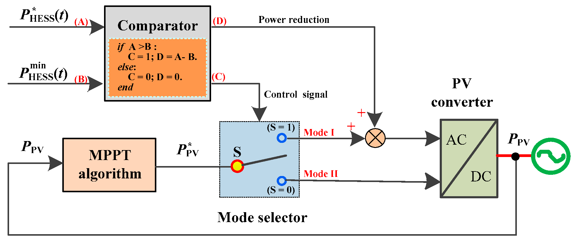
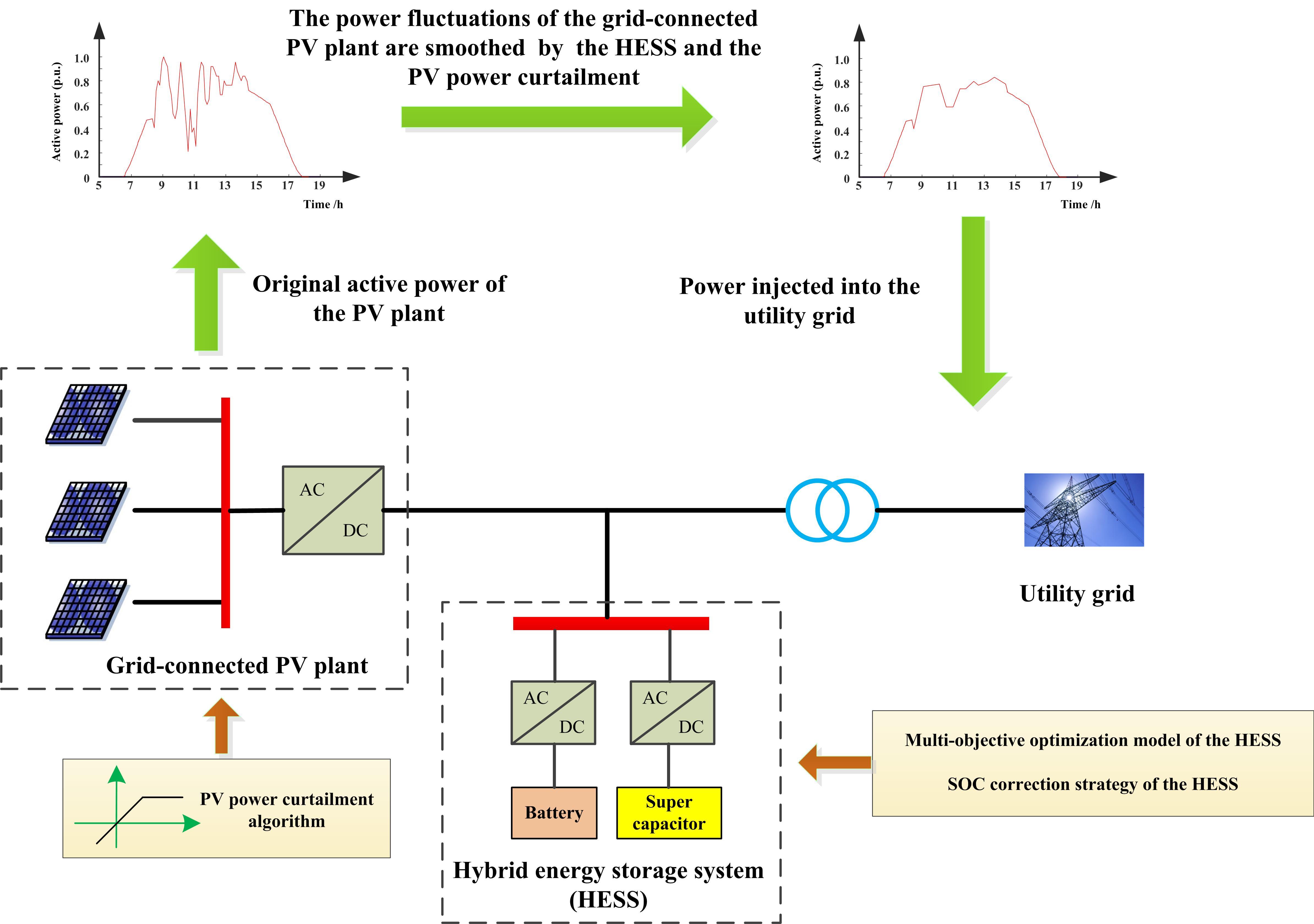
A control strategy for the HESS and PV is proposed to smooth power fluctuations of PV. When the power demand, which is used to smooth the upward power fluctuation, exceeds the maximum allowable power of the HESS, the excess power demand will be absorbed by reducing the PV power. Otherwise, only the HESS is used to smooth both the upward and downward power fluctuations.

(2)

A multi-objective optimization model is developed to dispatch the power demand of the HESS, which consists of two objectives: (1) To minimize the overall losses of the HESS; and (2) to keep the SOC of SCES fluctuating around 50%, considering the HESS needs to smooth the sudden changes in PV power. A simple prediction model is introduced to determine the weights of two sub-objective functions. Also, an SOC correction strategy is proposed to correct the SOCs of the HESS, when power fluctuations do not exceed the allowable limits.

(3)

According to 100 active power curves of a 750kW PV plant, numerous simulations are carried out to analyze the performances of the proposed smoothing strategies and the smoothing method of using the HESS [15]. Simulation results indicate that the performances of the proposed method are much better than the smoothing method of using the HESS.

This study contributes to the field of large-scale grid-connected PV applications. It is beyond the scope of this study to examine the allocation method of the HESS capacities.

This paper is structured as follows: Section 2 presents a general description of the power fluctuations of grid-connected PV plants. The details of the coordinated control strategy for the HESS and PV to smooth PV power fluctuations are discussed in Section 3, including the control strategies of the HESS and the PV power curtailment algorithm. Case studies and simulation results are presented in Section 4. The comprehensive performances of two different smoothing strategies are analyzed and discussed in Section 5. Finally, Section 6 presents the conclusions of this work.

2. Definition of the Power Fluctuations of a Grid-Connected PV Plant

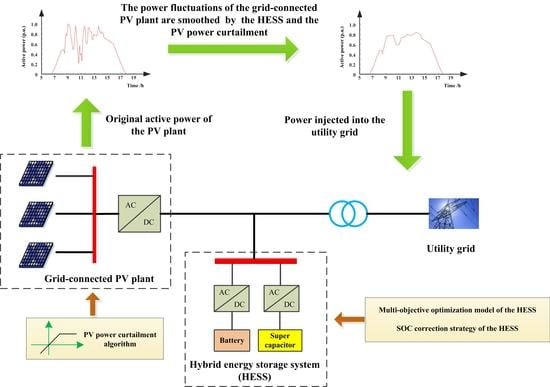
2.1. System Structures of a PV Plant

The system structures of a grid-connected PV plant with an HESS are shown in Figure 1. P_PV denotes the active power of PV, and C_pv denotes the installed capacity of a PV plant. The energy and power capacities of BES are denoted by E_BES and P_BES, respectively. The energy and power capacities of SCES are denoted by E_SCES and P_SCES, respectively. The SOCs of the battery and the supercapacitor are denoted by S₁ and S₂, respectively. The total power of the HESS is denoted by P_HESS, which is the sum of the BES power, P₁, and the SCES power, P₂. The power injected into the utility grid is denoted by P_Grid, and P_Grid = P_PV + P_HESS. In addition, the energy management system (EMS) monitors the real-time operating status of the system and controls the power of PV, BES, and SCES.

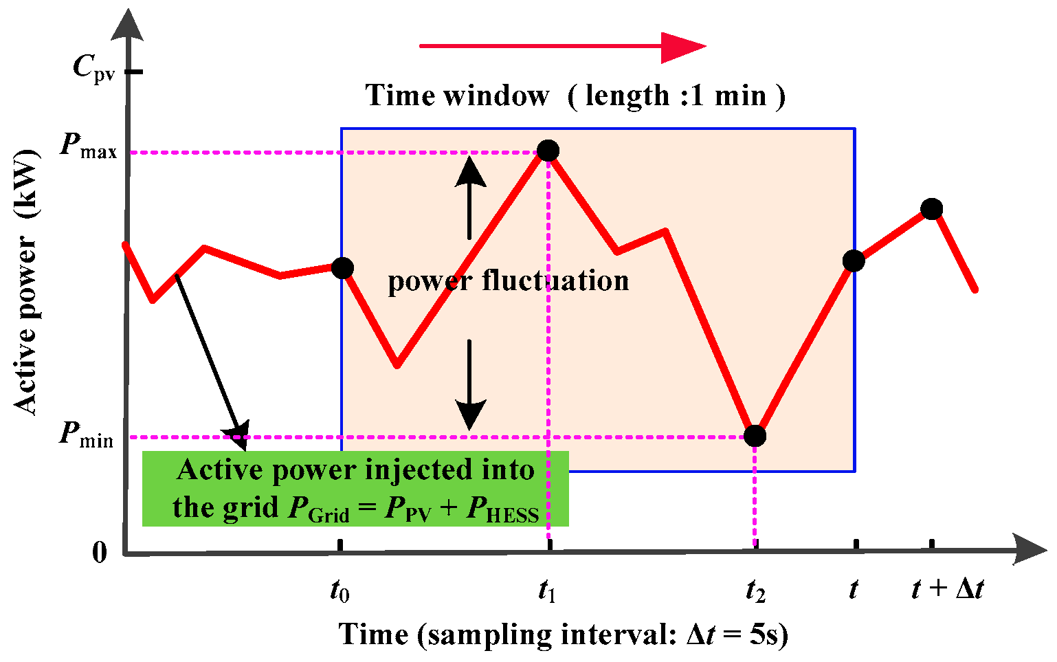
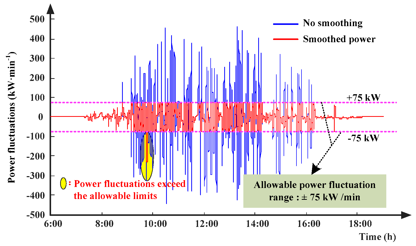
2.2. Definition of the PV Power Fluctuations

In this study, we mainly discuss the power fluctuation of PV in one minute. As shown in Figure 2, the power fluctuation can be defined as the difference between the maximum and minimum power values measured at the PCC in 1 min.

At time t, P_Grid,before(t) denotes the power value at the PCC if no correction action is provided, and P_Grid,after(t) denotes the power value at the PCC after providing the correction action. The power fluctuations of PV before and after the suppression are denoted by ΔP_Grid,before(t) and ΔP_Grid,after(t), respectively. According to the historical data of P_Grid, ΔP_Grid,before(t) can be calculated as follows:

$$\begin{array}{l}\Delta P_{\mathrm{Grid},\mathrm{before}}(t)=\{\begin{array}{l}\begin{array}{cc}{P}_{\max ,\mathrm{before}}(t)-P_{\min ,\mathrm{before}}(t),& i\ge j\end{array}\\ \begin{array}{cc}{P}_{\min ,\mathrm{before}}(t)-P_{\max ,\mathrm{before}}(t),& i<j\end{array}\end{array}\\ s.t. \{\begin{array}{l}\left[\begin{array}{cc}{P}_{\max ,\mathrm{before}}(t),& i\end{array}\right]=f_{\max }(A)\\ \left[\begin{array}{cc}{P}_{\min ,\mathrm{before}}(t),& j\end{array}\right]=f_{\min }(A)\\ A=\left\{P_{\mathrm{Grid}}(t_0),P_{\mathrm{Grid}}(t_0+\Delta t),\dots ,P_{\mathrm{Grid}}(t-\Delta t),P_{\mathrm{Grid},\mathrm{before}}(t)\right\}\\ t_0=t-1\min \end{array}\end{array}$$

(1)

where P_max,before(t) and P_min,before(t) represent the maximum and minimum values of the set A, respectively; i and j represent the indices of the maximum and minimum values of the set A, respectively; function [x, y] = f_max(·) returns the largest element of the input argument, where x and y denote the corresponding value and index of the largest element; function [x, y] = f_min(·) returns the value and index of the smallest element of the input argument; A is a set of power values measured at the PCC before the correction action is provided, and the time scale of the set A is 1 min; t₀ is the start time; Δt is the sampling interval and Δt = 5s.

In the same way, ΔP_Grid,after(t) can be calculated by (2) after the smoothing method is applied.

$$\begin{array}{l}\Delta P_{\mathrm{Grid},\mathrm{after}}(t)=\{\begin{array}{l}\begin{array}{cc}{P}_{\max ,\mathrm{after}}(t)-P_{\min ,\mathrm{after}}(t),& m\ge n\end{array}\\ \begin{array}{cc}{P}_{\min ,\mathrm{after}}(t)-P_{\max ,\mathrm{after}}(t),& m<n\end{array}\end{array}\\ s.t. \{\begin{array}{l}\left[\begin{array}{cc}{P}_{\max ,\mathrm{after}}(t),& m\end{array}\right]=f_{\max }(B)\\ \left[\begin{array}{cc}{P}_{\min ,\mathrm{after}}(t),& n\end{array}\right]=f_{\min }(B)\\ B=\left\{P_{\mathrm{Grid}}(t_0),P_{\mathrm{Grid}}(t_0+\Delta t),\dots ,P_{\mathrm{Grid}}(t-\Delta t),P_{\mathrm{Grid},\mathrm{after}}(t)\right\}\\ t_0=t-1\min \end{array}\end{array}$$

(2)

where B is a set of power values measured at the PCC after providing the correction action, and the time scale of the set B is 1 min; P_max,after(t) and P_min,after(t) represent the maximum and minimum values of the set B, respectively; m and n represent the indices of the maximum and minimum values of the set B, respectively.

2.3. Requirements of the Power Fluctuations of a Grid-Connected PV Plant

This paper assumes that the maximum fluctuation of power injected into the grid from PV should be less than 10 %C_pv/min, because this requirement is adopted by the PREPA to restrict the power fluctuations of PV [5]. Moreover, it is also adopted by the State Grid Corporation of China to restrict the fluctuations of wind power [16].

Therefore, ΔP_Grid,after needs to meet the following constraint:

$$\left|\Delta P_{\mathrm{Grid},\mathrm{after}}(t)\right|\le P_{\mathrm{limit}},\forall t\in T$$

(3)

where P_limit represents the maximum allowable power fluctuation of PV, hence P_limit = 10%C_pv; T is a set of sampling time, and T = {00:00, Δt, 2Δt, 3Δt,…, 24:00 - Δt, 24:00 h}.

3. Coordinated Control Strategy for the HESS and PV to Smooth PV Power Fluctuations

First, Section 3.1 describes the detailed flowchart of the proposed smoothing strategy. Then, the method used to control the PV power is discussed in Section 3.2. Finally, we explain the control strategies of the HESS in Section 3.3.

3.1. Flowchart of the Proposed Smoothing Strategy

This paper proposes a coordinated control strategy for the HESS and PV to smooth PV power fluctuations. The main ideas of this strategy consist of three aspects:

(1) Typically, when the PV power fluctuations do not exceed the maximum allowable power of the HESS, the proposed strategy only utilizes the HESS to smooth these power fluctuations while keeping the PV converter operating in the MPPT mode. Namely, the downward power fluctuations are smoothed by discharging (the HESS power is positive, P_HESS > 0), in contrast, the upward power fluctuations are smoothed by charging (the HESS power is negative, P_HESS < 0).

(2) However, if the upward power fluctuation exceeds the upper power limit of the HESS, the HESS will be charged using the maximum allowable power. At the same time, the excess power fluctuation will be absorbed by reducing the power generated by the PV converter.

(3) In addition, if the downward power fluctuation exceeds the lower power limit of the HESS, in this case, the HESS will be discharged using the maximum allowable power. Despite this, the power fluctuation of PV may not meet the requirements. However, this situation can be avoided by properly allocating the capacities of the HESS and controlling the SOCs of the HESS, which will be discussed later.

In summary, Figure 3 shows the flowchart of the proposed smoothing strategy, which consists of five key steps:

The first step, the EMS calculates the real-time power fluctuation of PV, ΔP_Grid,before(t), by (1), according to the real-time data, P_Grid,before(t), and the historical data of P_Grid.

The second step, according to the requirements of PV power fluctuations, the power demand of the HESS $P_{\mathrm{HESS}}^{*}(t)$, which is used to smooth the current power fluctuation, can be calculated by (4). Considering the constraints of the HESS, the maximum allowable charging and discharging power of HESS, which is denoted by $P_{\mathrm{HESS}}^{\min }$(t) and $P_{\mathrm{HESS}}^{\max }$(t), can be calculated by (5) and (6).

$$P_{\mathrm{HESS}}^{*}(t)=\{\begin{array}{ll}{P}_{\mathrm{limit}}-\Delta P_{\mathrm{Grid},\mathrm{before}}(t),\hfill & \Delta P_{\mathrm{Grid},\mathrm{before}}(t)>P_{\mathrm{limit}}\hfill \\ 0,\hfill & \left|\Delta P_{\mathrm{Grid},\mathrm{before}}(t)\right|\le P_{\mathrm{limit}}\hfill \\ -\left(P_{\mathrm{limit}}+\Delta P_{\mathrm{Grid},\mathrm{before}}(t)\right),\hfill & \Delta P_{\mathrm{Grid},\mathrm{before}}(t)<-P_{\mathrm{limit}}\hfill \end{array}$$

(4)

$$\{\begin{array}{l}{P}_{\mathrm{HESS}}^{\min }(t)=P_{\mathrm{BES}}^{\min }(t)+P_{\mathrm{SCES}}^{\min }(t)\\ P_{\mathrm{HESS}}^{\max }(t)=P_{\mathrm{BES}}^{\max }(t)+P_{\mathrm{SCES}}^{\max }(t)\end{array}$$

(5)

where $P_{\mathrm{BES}}^{\min }$(t) and $P_{\mathrm{BES}}^{\max }$(t) represent the maximum allowable charging and discharging power of BES, respectively; $P_{\mathrm{SCES}}^{\min }$(t) and $P_{\mathrm{SCES}}^{\max }$(t) represent the maximum allowable charging and discharging power of SCES, respectively. Moreover, $P_{\mathrm{BES}}^{\min }$(t), $P_{\mathrm{BES}}^{\max }$(t), $P_{\mathrm{SCES}}^{\min }$(t), and $P_{\mathrm{SCES}}^{\max }$(t) can be calculated as follows:

$$\{\begin{array}{l}{P}_{\mathrm{BES}}^{\min }(t)=\max \left\{\left(S_1(t)-S_{1,\max }\right)E_{\mathrm{BES}}/\Delta t, -P_{\mathrm{BES}}\right\}\\ P_{\mathrm{BES}}^{\max }(t)=\min \left\{\left(S_1(t)-S_{1,\min }\right)E_{\mathrm{BES}}/\Delta t, P_{\mathrm{BES}}\right\}\\ P_{\mathrm{SCES}}^{\min }(t)=\max \left\{\left(S_2(t)-S_{2,\max }\right)E_{\mathrm{SCES}}/\Delta t, -P_{\mathrm{SCES}}\right\}\\ P_{\mathrm{SCES}}^{\max }(t)=\min \left\{\left(S_2(t)-S_{2,\min }\right)E_{\mathrm{SCES}}/\Delta t, P_{\mathrm{SCES}}\right\}\end{array}$$

(6)

where the functions of max{x₁, x₂} and min{x₁, x₂} return the maximum and minimum values between x₁ and x₂, respectively; S_1,max, and S_1,min are the upper and lower limits of the SOC of the battery, respectively; S_2,max, and S_2,min are the upper and lower limits of the SOC of the supercapacitor, respectively; in this work, S_1,min = 20%, S_1,max = 90%, S_2,min = 5%, and S_2,max = 100%.

The third step, according to the power demand of the HESS $P_{\mathrm{HESS}}^{*}$(t) and the maximum power capacity of the HESS, the EMS needs to determine whether to limit the PV power and calculate the actual power command of the HESS. Therefore, a PV power curtailment algorithm is developed to control the PV power, and the details of this algorithm are discussed in the following section.

In addition, after implementing the PV power curtailment algorithm, the power demand of HESS, $P_{\mathrm{HESS}}^{*}$(t), needs to be modified, and the modified power demand is denoted by $P_{\mathrm{HESS},\mathrm{M}}^{*}$(t), which is calculated and explained in Section 3.2.

The fourth step, the HESS can respond immediately after receiving the real power command. There are two possible situations:

(1) If the modified power demand, $P_{\mathrm{HESS},\mathrm{M}}^{*}$(t), is not zero, the $P_{\mathrm{HESS},\mathrm{M}}^{*}$(t) will be allocated to BES and SCES using the multi-objective optimization model, which is discussed in Section 3.3.1.

(2) On the other hand, if $P_{\mathrm{HESS},\mathrm{M}}^{*}$(t) is zero, there is no need for the HESS to output power to smooth the current power fluctuation. Therefore, an SOC correction strategy of the HESS is developed to correct the SOCs of BES and SCES, because their SOCs may approach the lower limits due to the PV power curtailment and operating losses of the HESS. The details of this strategy are discussed in Section 3.3.5.

Finally, the EMS sends the power commands to the PV converter, the BES converter, and the SCES converter. Through the close cooperation between the PV converter and the HESS, the power fluctuation at time t will meet the requirements. After that, the EMS will start the next control loop and repeat the above-described steps.

3.2. PV Power Curtailment Algorithm

Reducing the reference power value generated by the MPPT algorithm (e.g., the hill climbing method [17]) can easily restrict the upward power fluctuation of PV. Therefore, the PV power curtailment algorithm proposed in this paper is shown in Figure 4.

The main control processes of this algorithm are as follows:

When the power demand of the HESS used to smooth the upward power fluctuation is greater than the maximum allowable charging power of the HESS, i.e., $P_{\mathrm{HESS}}^{*}$(t) < $P_{\mathrm{HESS}}^{\min }$(t), the excess power demand is absorbed by reducing the PV power. The comparator controls the output status of the mode selector, if $P_{\mathrm{HESS}}^{*}$(t) < $P_{\mathrm{HESS}}^{\min }$(t), then the comparator (port C) outputs signal “1”, thus the mode selector switches from mode II to mode I. Consequently, the actual power of the PV converter is reduced by |$P_{\mathrm{HESS}}^{*}$(t) - $P_{\mathrm{HESS}}^{\min }$| compared to the original power, $P_{\mathrm{PV}}^{*}$(t), which is calculated by the MPPT algorithm, such as the hill climbing method [17]. Otherwise, there is no need to reduce the PV power, and the actual power of PV is equal to $P_{\mathrm{PV}}^{*}$(t).

This section has discussed how to control the PV power, according to the real-time state of the HESS and the power demand of the HESS, $P_{\mathrm{HESS}}^{*}$(t). After the implementation of the PV power curtailment algorithm, the $P_{\mathrm{HESS}}^{*}$(t) needs to be modified due to the constraints of the HESS. Therefore, the modified power demand of HESS is denoted by $P_{\mathrm{HESS},\mathrm{M}}^{*}$(t), which can be calculated as follows:

(1) If $P_{\mathrm{HESS}}^{*}$(t) < $P_{\mathrm{HESS}}^{\min }$(t), the original power demand will be reduced to $P_{\mathrm{HESS}}^{\min }$(t) by limiting the power generated by PV.

(2) If $P_{\mathrm{HESS}}^{*}$(t) > $P_{\mathrm{HESS}}^{\max }$(t), the original power demand will be reduced to $P_{\mathrm{HESS}}^{\max }$(t).

(3) If $P_{\mathrm{HESS}}^{*}$(t) does not exceed the allowable limits of the HESS at time t, the power demand will not be changed.

$$P_{\mathrm{HESS},\mathrm{M}}^{*}(t)=\{\begin{array}{l}\begin{array}{cc}{P}_{\mathrm{HESS}}^{\min }(t),& P_{\mathrm{HESS}}^{*}(t)<P_{\mathrm{HESS}}^{\min }(t)\end{array}\\ \begin{array}{cc}{P}_{\mathrm{HESS}}^{*}(t),& P_{\mathrm{HESS}}^{\min }(t)\le P_{\mathrm{HESS}}^{*}(t)\le P_{\mathrm{HESS}}^{\max }(t)\end{array}\\ \begin{array}{cc}{P}_{\mathrm{HESS}}^{\max }(t),& P_{\mathrm{HESS}}^{*}(t)>P_{\mathrm{HESS}}^{\max }(t)\end{array}\end{array}$$

(7)

Having determined the total power that BES and SCES need to output, this paper will now move on to discuss the control strategy of the HESS.

3.3. Control Strategy of the HESS

The control strategy of the HESS consists of two keys aims: (1) To optimize the power between BES and SCES; and (2) to correct the SOCs of the battery and the supercapacitor. The specific explanations are as follows:

First, if $P_{\mathrm{HESS},\mathrm{M}}^{*}$(t) is not equal to zero, it indicates that the HESS is required to absorb the excess power fluctuation by charging or discharging. Therefore, this paper establishes a multi-objective optimization model to optimize the power of the HESS, considering the overall losses of the HESS and the SOC optimization of SCES.

On the other hand, the HESS does not need to smooth PV power fluctuations when $P_{\mathrm{HESS},\mathrm{M}}^{*}$(t) is equal to zero. Therefore, this paper proposes an SOC correction strategy of HESS to actively control the SOCs of BES and SCES. Because of the PV power curtailment, the total energy absorbed by the HESS may be less than the total energy released. As a result of this, the SOCs of the HESS will gradually decrease and even exceed their lower limits. That has bad effects on smoothing the following power fluctuations. Therefore, a method is needed to improve the SOCs of BES and SCES, once their SOCs are below certain limits.

In the section that follows, first, we carefully describe the objective functions, constraints, and solution algorithms of the multi-objective optimization model of the HESS, which is used to optimize the power between BES and SCES. Then, we explain the details of the SOC correction strategy of the HESS.

3.3.1. Multi-Objective Optimization Model of the HESS

In the problem of dispatching the power of the HESS, this paper mainly considers the losses of the HESS and the SOC optimization of SCES.

First, the operating losses of two energy storage systems are different, because the comprehensive efficiencies of BES and SCES are different. The efficiency of BES (Li-ion battery) is about 85%—90% [14], and the efficiency of SCES is about 90%—95% [14]. Therefore, to minimize the overall losses of systems, the efficiencies of the HESS should be considered.

On the other hand, the energy capacity of SCES is usually configured to be smaller, and the power capacity of SCES is usually configured to be larger because of the high costs and high power rates of the supercapacitor [14]. Moreover, the lifetime of the supercapacitor is much longer than that of the battery, for example, the number of cycles of the supercapacitor is about 10 to 100 times that of the Li-ion battery [14]. Therefore, to fully exploit the characteristics of the supercapacitor, the SCES is encouraged to absorb more components of the PV power fluctuations. However, the SOC of SCES can easily reach the upper or lower limits due to the smaller energy capacity of SCES. Therefore, it is expected that the SOC of SCES can fluctuate around 50%, ensuring that the SCES has sufficient remaining capacity to cope with sudden changes in PV power.

Consequently, the multi-objective optimization model of the HESS is described in (8). The optimization variable is x, which consists of the BES power, P₁, and the SCES power, P₂. f₁(x) and f₂(x) are sub-objective functions, where f₁(x) aims to minimize the overall losses of the HESS, and f₂(x) aims to optimize the SCES SOC. h(x) and g(x) are the equality and inequality constraints of the model, respectively.

$$\begin{array}{l}\underset{x\in {\mathrm{R}}^2}{\min } \left[f_1(x),f_2(x)\right]\\ s.t.\{\begin{array}{l}x={\left[P_1,P_2\right]}^{\mathrm{T}}\\ h(x)=0\\ g(x)\le 0\end{array}\end{array}$$

(8)

Before solving this model, the mathematical models of f₁(x), f₂(x), h(x), and g(x) should be presented.

3.3.2. Objective Functions and Constraints

(a) Sub-objective function, f₁(x).

The losses of the HESS consist of operating losses of BES and SCES. To simplify the analysis, this paper uses the charging and discharging power to evaluate the losses of the HESS. Therefore, the sub-objective function, f₁(x), can be described as follows:

$$\min f_1\left(P_1(t),P_2(t)\right)=\Delta t\left[\left|P_1(t)\right|(1-{\eta }_1)+\left|P_2(t)\right|(1-{\eta }_2)\right]$$

(9)

where η₁ and η₂ are the efficiencies of BES and SCES, respectively, in this work, η₁ = 90% and η₂ = 95% [18,19].

(b) Sub-objective function, f₂(x).

To minimize the deviation between the SOC of SCES and the reference value of SOC (50%), the sub-objective function, f₂(x), can be described as follows:

$$\min f_2\left(P_1(t),P_2(t)\right)=\frac{\left|S_2(t-\Delta t)-P_2(t)\Delta t/E_{\mathrm{SCES}}-50\%\right|}{\Delta S_{2,\max }}$$

(10)

where ΔS_2,max represents the maximum difference between the SCES SOC and its reference value (50%). ΔS_2,max can be determined according to the upper and lower limits of the SCES SOC, and ΔS_2,max = max{S_2,max – 50%, 50% – S_2,min}. In this work, S_2,max = 100%, and S_2,min = 5%, hence ΔS_2,max is 50%.

To solve the above-established optimization model, the multi-objective optimization model is transformed into a single-objective optimization model, as shown in (11). Since the value of the sub-objective function, f₂(x), is [0, 1], no standardization is required.

Objective function:

$$\min \lambda \frac{f_1\left(P_1(t),P_2(t)\right)-f_{1,\min }}{f_{1,\max }-f_{1,\min }}+\left(1-\lambda \right)f_2\left(P_1(t),P_2(t)\right)$$

(11)

where λ is the weight, and 0 ≤ λ ≤ 1; f_1,min and f_1,max are the minimum and maximum values of the sub-objective function, f₁, respectively. In addition, the value of weight, λ, is discussed in the following section.

Constraints:

$$P_1(t)+P_2(t)=P_{\mathrm{HESS},\mathrm{M}}^{*}(t)$$

(12)

$$\{\begin{array}{l}-P_{\mathrm{BES}}\le P_1(t)\le P_{\mathrm{BES}}\\ -P_{\mathrm{SCES}}\le P_2(t)\le P_{\mathrm{SCES}}\end{array}$$

(13)

$$\{\begin{array}{l}{S}_{1,\min }\le S_1(t)-\frac{P_1(t)\Delta t}{E_{\mathrm{BES}}}\le S_{1,\max }\\ S_{2,\min }\le S_2(t)-\frac{P_2(t)\Delta t}{E_{\mathrm{SCES}}}\le S_{2,\max }\end{array}$$

(14)

$$P_1(t)P_2(t)\ge 0$$

(15)

The constraints consist of four parts:

(1) Constraint (12) states that the sum of P₁(t) and P₂(t) should equal to $P_{HESS,\mathrm{M}}^{*}$(t) determined by (7).

(2) Constraint (13) requires that the power of BES and SCES cannot exceed their maximum power capacities.

(3) The SOC constraints of the HESS are described in (14).

(4) Constraint (15) indicates that the directions of the power flow of BES and SCES cannot be reversed. For example, BES cannot be charged while SCES is discharging.

3.3.3. Calculation Method of the Weight, λ

In this optimization problem, there is a trade-off between reducing the losses of the HESS and improving the ability of the HESS to cope with the sudden changes in PV power. It is more preferred to use SCES to respond to the power demand of the HESS when the weight, λ, tends to zero, achieving minimum system losses. However, the variation of the SCES SOC will increase, and the mean SOC of SCES will be farther from the reference SOC (50%). Hence, the sudden power fluctuations of PV may not be smoothed completely. On the other hand, the SOC deviation of SCES will decrease when the weight, λ, tends to 1. Hence, the HESS can respond quickly to the sudden power fluctuations of PV. However, the power and frequency of BES will increase, resulting in increased system losses and a reduced service life of BES.

Therefore, this paper dynamically adjusts the value of the weight, λ, using the short-term prediction model, which is used to predict the HESS’s energy demand for smoothing the downward power fluctuation, as shown in Figure 5. Note that the energy demand of smoothing the upward power fluctuation is not considered, because the upward power fluctuation can be smoothed by limiting the PV power. An explanation of this control is as follows:

If the PV power is suddenly declined, the HESS needs to be continuously discharged for a while (see Figure 5). However, if the weight, λ, is always fixed, the energy stored in SCES will be quickly emptied, thereby losing the ability to compensate. Actually, in this case, the BES should participate in smoothing that downward power fluctuation as early as possible, rather than starting to discharge when the remaining energy in SCES approaches zero.

Overall, the weight, λ, is usually set to 0.7, which is obtained by the analytic hierarchy process (AHP) method [20]. Of course, λ can be flexibly adjusted within the range of 0 to 1 according to the actual applications. However, once the HESS’s energy demand of smoothing the downward power fluctuation, which is denoted by E_need(t) and calculated by (16), is greater than 50% of the remaining energy in SCES, then the weight, λ, will be set to 0, otherwise the weight, λ, will always be equal to 0.7.

A short-term prediction mode of E_need(t) is shown as Figure 5. When PV power suddenly drops at time t, E_need(t) (i.e., green shaded areas in Figure 5) can be predicted as follows:

$$\{\begin{array}{l}{T}_{\mathrm{delay}}=\mathrm{ceil}\left(\frac{P_{\mathrm{Last}}^{\max }(t)-P_{\mathrm{PV}}(t)}{P_{\mathrm{limit}}}\right)-1, P_{\mathrm{Last}}^{\max }(t)>P_{\mathrm{PV}}(t)\\ E_{\mathrm{need}}(t)={\displaystyle \underset{t}{\overset{t+n\Delta t}{\int }}\left(P_{\mathrm{Grid}}(t)-P_{\mathrm{PV}}(t)\right)d}t\end{array}$$

(16)

where T_delay is the total time that the HESS will be discharged continuously; $P_{\mathrm{Last}}^{\max }$(t) represents the maximum power of PV in the past minute; function ceil(x) rounds x to the nearest integer greater than or equal to x; n = T_delay/Δt.

In addition, the prediction model described in (16) is a rather simple prediction strategy. One reason why we did not choose the more advanced tools, such as model predictive control (MPC), is as follows: The advanced tools require a lot of historical data and computation time, which may reduce the real-time performance of the system because this study sets the sampling time to 5 s. Although the prediction method proposed in this paper is simple, the calculation speed is very fast, and the simulation results also proved the effectiveness of the method. Of course, if there is a higher requirement for prediction accuracy, the proposed method may not work. Thus, more advanced prediction tools, such as MPC, can be used.

3.3.4. Solution Method

This paper uses the IBM ILOG CPLEX solver developed by the International Business Machines Corporation (IBM) to solve the multi-objective optimization model [21]. The optimization model established in this paper is standard nonlinear programming. Thus, many algorithms can easily solve this problem, such as the artificial intelligence algorithms: Particle Swarm Optimization (PSO) and Genetic Algorithm (GA)-[22]. Considering the speed of calculation and the convenience of programming, this paper uses the CPLEX solver to optimize the established model, because it can be called in MATLAB and has good convergence.

3.3.5. SOC Correction Strategy of the HESS

The main idea of the SOC correction strategy of the HESS is that SCES and BES will be charged when the power demands of the HESS used to smooth PV power fluctuations are equal to zero (i.e., $P_{\mathrm{HESS},\mathrm{M}}^{*}$(t) = 0). The specific rules for correcting the SOCs of SCES and BES are as follows:

First, the general principle is that SCES will be charged first until its SOC is greater than 30%. Obviously, the charging process is discontinuous, because the HESS SOCs are corrected only when PV power fluctuations do not exceed the limits and the HESS does not need to provide a correction action. Second, if the SOC of SCES is greater than 30%, indicating that SCES does not need to be corrected, then BES will be charged if its SOC is less than 30%. Otherwise, there is no need to correct the BES SOC. Finally, the charging power needs to meet the constraint described in (17), because the current power fluctuation of PV may exceed the limits due to the additional charging power. Also, the charging power needs to meet the constraints described in (13).

$$\{\begin{array}{l}{P}_{\mathrm{charge}}(t)=-\left[P_{\mathrm{PV}}(t)-\left(P_{\max ,\mathrm{before}}(t)-P_{\mathrm{limit}}\right)\right]\\ s.t. P_{\mathrm{HESS},\mathrm{M}}^{*}(t)=0\end{array}$$

(17)

where P_charge(t) is the maximum charging power that can be used to charge SCES or BES.

4. Case Studies

In this section, first, three typical scenarios that represent the general cases of PV power fluctuations are established. Then, taking these typical scenarios as an example, the proposed smoothing strategy is verified by numerous simulations. Finally, we analyze the impacts of the PV power curtailment algorithm and the SOC correction strategy on smoothing PV power fluctuations.

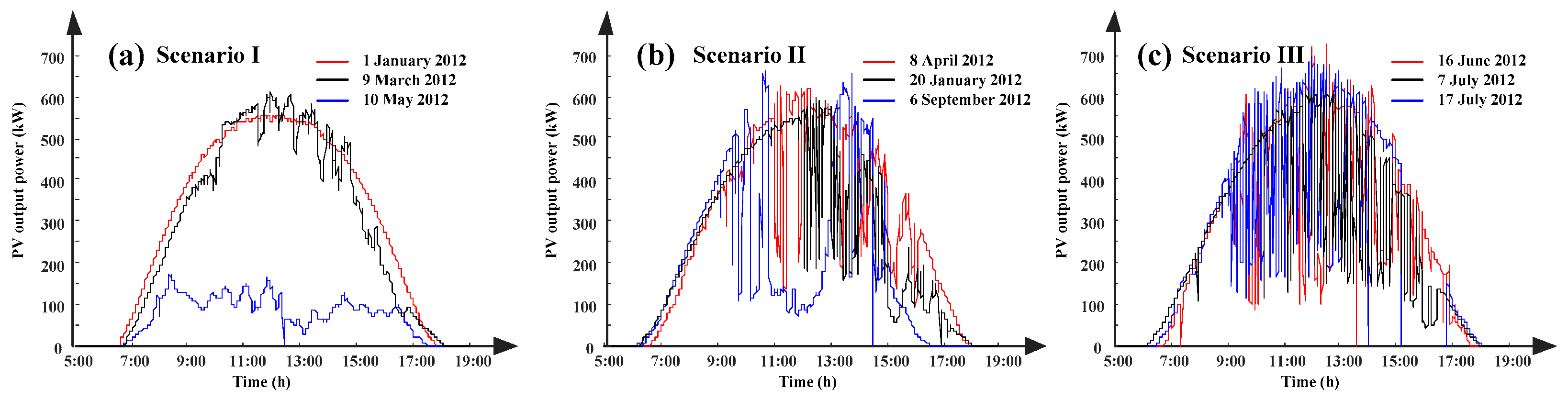
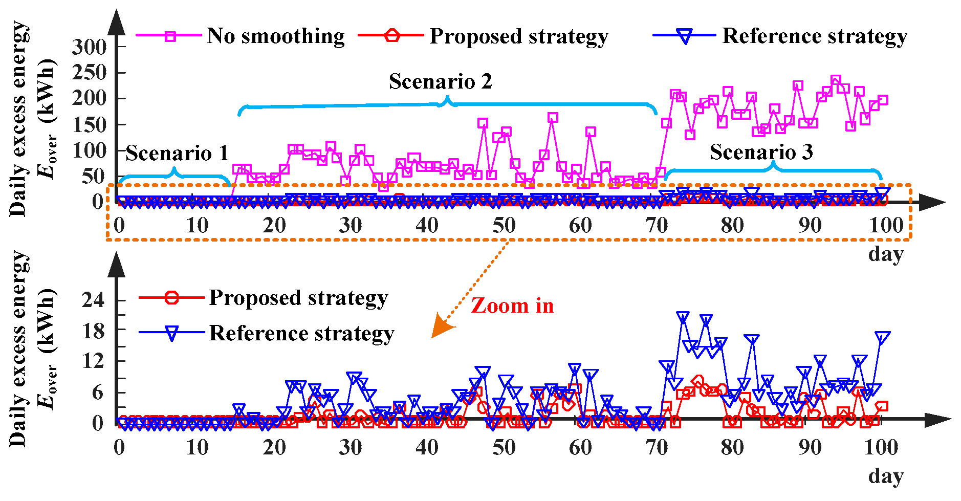
4.1. Typical Scenarios of PV Power Fluctuations

Based on the database that recorded the active power data of a 750 kW PV plant for one year, these daily active power curves of PV can be divided into three main categories using the k-means clustering algorithm [23]: (1) Scenario I; (2) scenario II; and (3) scenario III, as shown in Figure 6. Due to the limited size of the figure, only three daily power curves were plotted in each scenario.

Among these scenarios, the power fluctuations in scenario I are minimal because it represents the power generated by PV on sunny or rainy days. Scenario III has the worst power fluctuations because the power is generated by PV on cloudy days. Also, the statistical results indicate that scenario II is the most common cases of PV power fluctuations. Therefore, the probability of scenario II is also the highest, accounting for 56% (204 days) of the year. Moreover, the probabilities of scenario I and scenario III are 15% (55 days) and 29% (106 days), respectively.

4.2. Simulation and Analysis

Before starting simulations, it is necessary to set simulation parameters, such as the energy and power capacities of BES and SCES, and the initial SOCs of BES and SCES. However, this paper mainly focuses on how to dispatch the power of the HESS after the capacities of the HESS have been determined, and the optimal allocation of the HESS will be discussed carefully in the following research. Therefore, according to previous studies [15,16,24], the simulation parameters were configured as shown in

Table 1. Simulation parameters.

Parameters	Symbols	Values
Energy capacity of BES	EBES	100 (kWh)
Power capacity of BES	PBES	50 (kW)
Energy capacity of SCES	ESCES	17 (kWh)
Power capacity of SCES	PSCES	400 (kW)
Initial SOC of BES	--	90%
Initial SOC of SCES	--	50%
Capacity of the PV plant	CPV	750 (kWp)
Requirements of power fluctuations	Plimit	75 (kW/min)

.

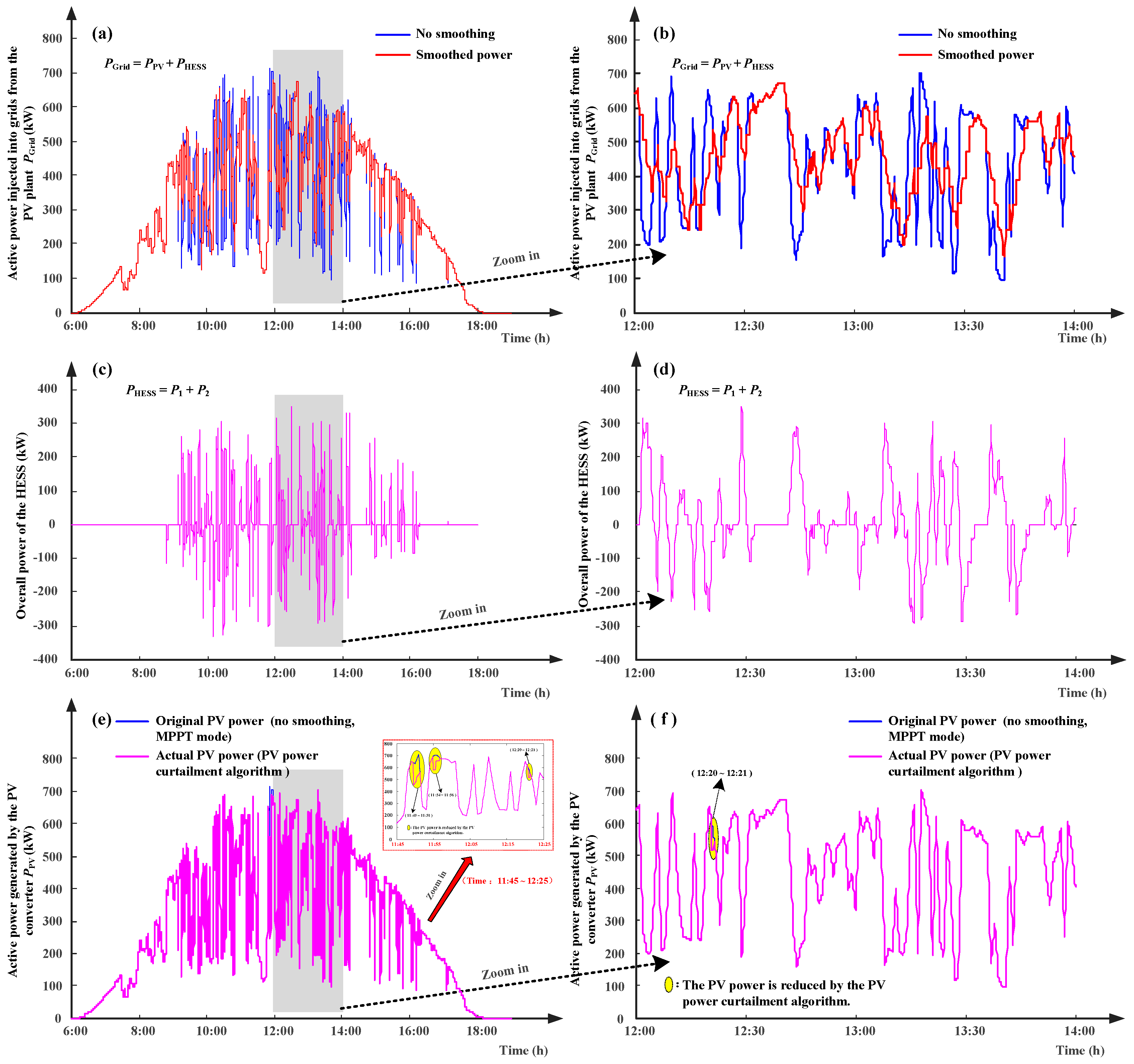
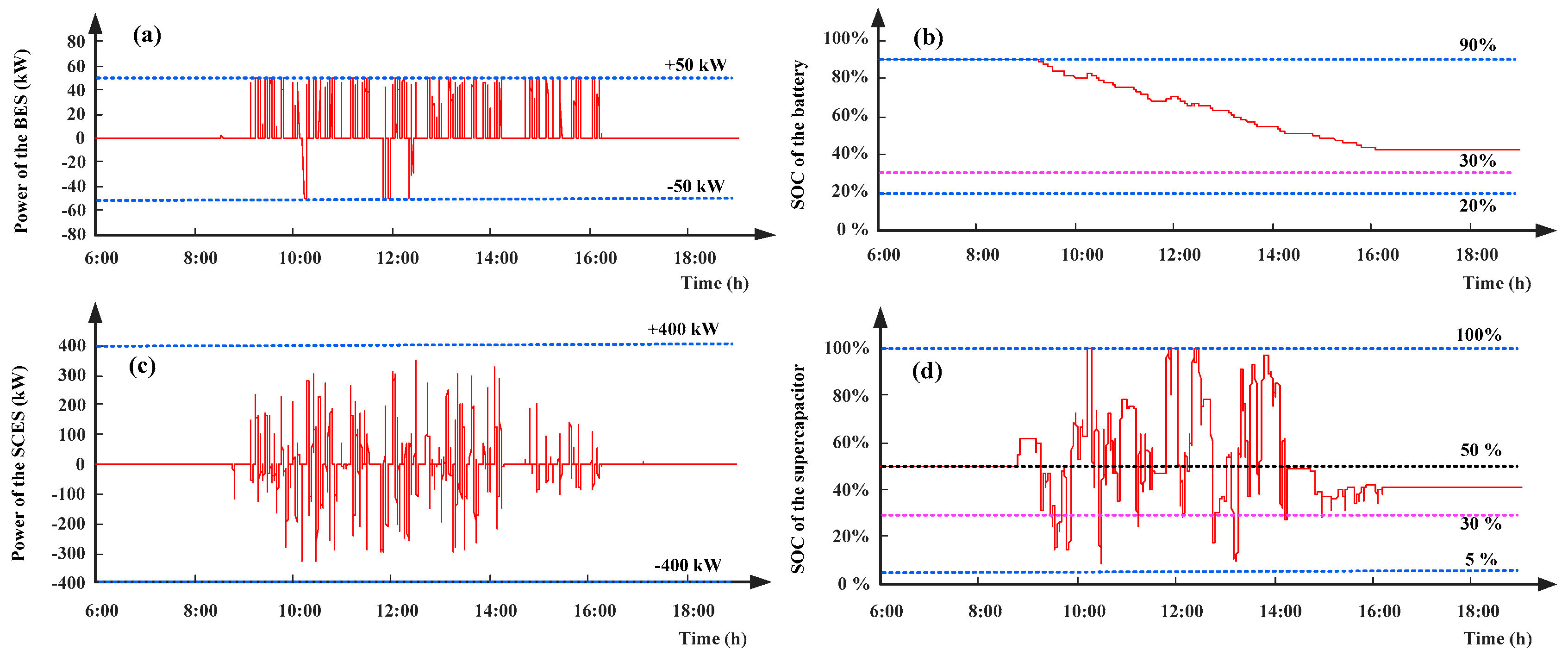
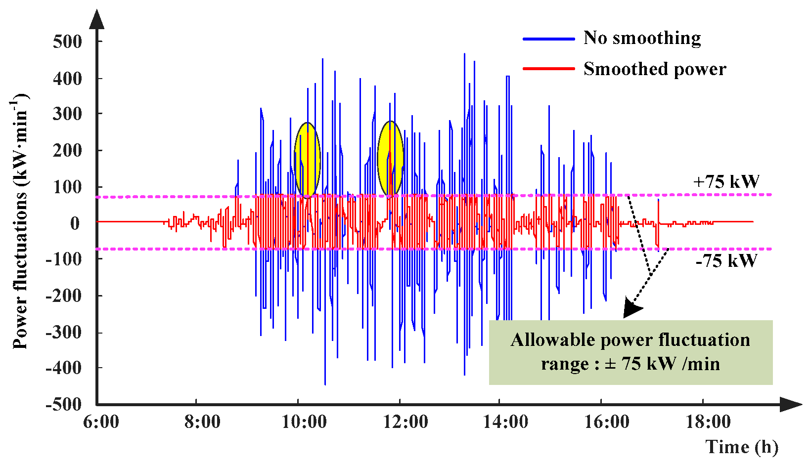
4.2.1. Performances of the Proposed Smoothing Strategy

The worst scenario of PV power fluctuations (i.e., scenario III) was chosen to verify the correctness and effectiveness of the proposed smoothing strategy. Figure 7 shows the active power injected into the utility grid from the PV plant (i.e., P_Grid), the overall power of the HESS (i.e., P_HESS), and the power generated by the PV converter (i.e., P_PV). Moreover, the fluctuations of the power injected into the grid before and after the suppression can be calculated by (1) and (2), respectively, as shown in Figure 8.

As can be seen from Figure 7a,b, and Figure 8, after the suppression, the power fluctuations of the grid-connected PV plant are significantly reduced. The results, as shown in Figure 8, indicate that the PV power fluctuations (solid red line) fully meet the requirements described in (3), although the original power fluctuations (solid blue line) are quite serious. The simulation results demonstrate that the proposed smoothing strategy can effectively smooth the power fluctuations of grid-connected PV plants.

It can be seen from Figure 7c,d that the HESS can accurately track the changes in PV power and provide the correct compensation power. Moreover, the PV power curtailment algorithm can effectively reduce the power generated by the PV converter, as shown in Figure 7e,f, when the HESS is unable to fully absorb the upward power fluctuation of PV. Simulation results demonstrate that the proposed method can correctly control the power of the HESS and the PV converter and ensure that the power injected into the utility grid from PV plants can meet the requirements.

Figure 9 shows the power and SOC profiles of the HESS. As can be seen from Figure 9a,c, the power provided by SCES is significantly larger than that of BES because the objective of reducing the losses of the HESS is considered, while allocating the total power demand, $P_{\mathrm{HESS},\mathrm{M}}^{*}$. It can be seen from Figure 9d that the SOC of SCES fluctuates around the reference value of 50%. Although the amplitude of the fluctuation is large, it is still within the allowable range because we also consider the SCES SOC optimization, while optimizing the power demand of the HESS. In summary, these results indicate that the established multi-objective optimization model can correctly dispatch the power of the HESS.

In addition, the SOCs of BES and SCES need to be adjusted to the initial states, i.e., S₁ = 90% and S₂ = 50%, during the night (00:00—5:00), because the HESS needs to smooth the power fluctuations of the next day. Although all the simulations are conducted on data obtained from a 750 kW PV plant, the idea of the proposed smoothing method can also be used in various PV plants. However, it is necessary to properly allocate the energy and power capacities of the HESS, according to the capacity of PV plants and the requirements of power fluctuations, and these studies are ongoing.

4.2.2. Impacts of the PV Power Curtailment Algorithm on Smoothing Power Fluctuations

To verify the effectiveness of the PV power curtailment algorithm, another simulation was done based on the same case studied in Section 4.2.1. This simulation did not use the PV power curtailment algorithm. However, only the HESS was used to smooth power fluctuations. As a result, the power fluctuation profiles are shown in Figure 10.

As can be seen from Figure 10, some fluctuations highlighted by yellow circles exceed the upper limit. In contrast, the power fluctuations shown in Figure 8 are completely within the allowable limits. Therefore, the PV power curtailment algorithm helps the HESS to achieve better smoothing results. Of course, we can also achieve the same results by increasing the capacities of the HESS, but it will significantly increase the initial investment costs of the HESS.

4.2.3. Impacts of the SOC Correction Strategy of the HESS on Smoothing Power Fluctuations

This section also used the case discussed in Section 4.2.1, but this simulation did not implement the SOC correction strategy of the HESS. As a result, the power fluctuation profiles are shown in Figure 11, and the SOC profiles are shown in Figure 12.

As can be seen from Figure 11, some power fluctuations, which are highlighted by yellow circles, exceed the lower limit. Because, at those moments, the SOCs of SCES reach the lower limit, the HESS can no longer be discharged to smooth those power fluctuations. However, if the SOC correction strategy is applied, SCES and BES will be charged if their SOC is below 30%. As shown in Figure 12b, the SOC of SCES (solid red line) is corrected several times, such as around 9:40. Overall, it can be seen from Figure 12 that the corrected SOC profiles of BES and SCES (solid red lines) are higher sometimes compared to the uncorrected SOC profiles (solid blue lines).

In summary, these results indicate that the proposed SOC correction strategy can effectively correct the SOCs of the HESS, and it is advantageous for the HESS to smooth PV power fluctuations.

5. Comparison of Two Smoothing Strategies

To evaluate the advantages and disadvantages of the proposed strategy, this paper compares it with a strategy developed in [15]. The reference strategy also uses the HESS to smooth PV power fluctuations, but it does not control the power of PV, but keeps the PV converter operating in the MPPT mode.

In the simulations discussed in Section 4.2, the energy and power capacities of the HESS were set to 17 kWh/400 kW (see Table 1). Therefore, the simulation parameters of the reference strategy are also set to be the same as the proposed strategy, as shown in

Table 2. Energy and power capacities of the HESS of the two smoothing strategies.

Strategies	EBES (kWh)	PBES (kW)	ESCES (kWh)	PSCES (kW)
Reference strategy [15]	100	50	17	400
Proposed strategy	100	50	17	400

.

5.1. Performances of Smoothing Power Fluctuations

To evaluate the performances of the above two strategies in various scenarios, 100 PV power curves were selected from Figure 6, including 15 curves selected from scenario I, 56 curves selected from scenario II, and 29 curves selected from scenario III.

After the suppression, the excess power fluctuation is denoted by P_over, as shown in (18). Therefore, the daily excess energy, which is denoted by E_over, can be calculated by (19). After the suppression, the smaller the value of E_over, the better the performance of the smoothing power fluctuations.

$$P_{\mathrm{over}}(t)=\{\begin{array}{ll}0,& \left|\Delta P_{\mathrm{Grid},\mathrm{after}}(t)\right|\le P_{\mathrm{limit}}\\ \left|\Delta P_{\mathrm{Grid},\mathrm{after}}\right|-P_{\mathrm{limit}},& \left|\Delta P_{\mathrm{Grid},\mathrm{after}}(t)\right|>P_{\mathrm{limit}}\end{array})$$

(18)

$$E_{\mathrm{over}}=\Delta t{\displaystyle \sum _{t=00:00}^{24:00}{P}_{\mathrm{over}}(t)}$$

(19)

Therefore, when two smoothing strategies are applied to these 100 cases, the profiles of E_over are shown in Figure 13.

The results demonstrate that the performance of the proposed smoothing strategy is better because the daily excess energy (E_over) is significantly less than that of the reference strategy. In fact, when E_over is equal to zero, it means that the power fluctuations after the suppression are completely satisfactory. However, in some cases, E_over is not equal to zero. One explanation of these results is that the HESS capacities were determined based on the case discussed in Section 4.2, and for other cases, the capacities may be a little smaller. Note that the capacity allocation of the HESS is beyond the scope of this paper.

In conclusion, under the same conditions (such as capacities of the HESS, requirements of power fluctuations, and the installed capacity of the PV plant), combining the HESS and the PV power curtailment has better performances of smoothing PV power fluctuations than the method of using the HESS.

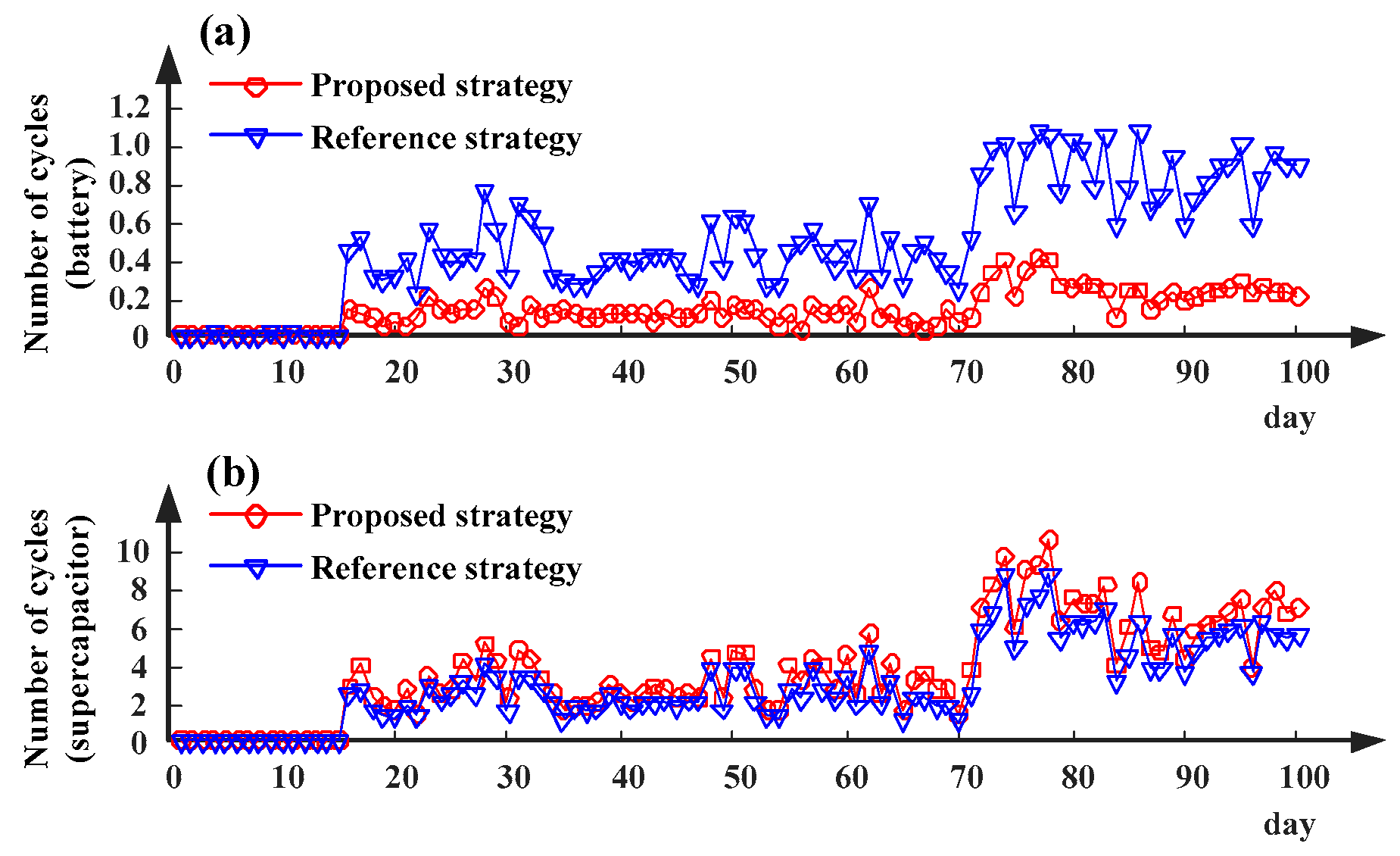
5.2. Lifetime Aging of Batteries and Supercapacitors.

To analyze the lifetime aging of batteries and supercapacitors, the 100% depth of the discharge (DOD) equivalent model developed in [25] was used to evaluate the lifetime aging of batteries, as shown in (20). Moreover, the energy throughput model defined by (21) was used to evaluate the lifetime aging of the supercapacitor.

$$n_{\mathrm{bat},\mathrm{eq}}={{\displaystyle \sum _{i=2}^{m}0.5\left(\left|S_{1,i}-S_{1,i-1}\right|\right)}}^{k_p}$$

(20)

where n_bat,eq is the 100% DOD equivalent cycles of a battery; m represents the number of extreme points of the battery’s SOC curve, i.e., S₁(t), t∈T; S_1,i is the SOC value at the extreme point i; k_p is a constant, 0.8 ≤ k_p ≤ 2.1, in this work, k_p = 0.976 [25,26].

$$n_{\mathrm{cap},\mathrm{eq}}=\left(\Delta t{\displaystyle \sum _{t=00:00}^{24:00}\left|P_2(t)\right|}\right)/\left(2E_{\mathrm{SCES}}\right)$$

(21)

where n_cap,eq is the equivalent cycles of the supercapacitor.

Therefore, when two smoothing strategies are applied to these 100 cases, the profiles of n_bat,eq, and n_cap,eq are shown in Figure 14.

As can be seen from Figure 14, it is apparent that the battery cycles of the proposed smoothing strategy are smaller than that of the reference strategy. Therefore, these results indicate that the PV power curtailment can reduce the number of cycles of the battery while using the HESS to smooth PV power fluctuations.

In conclusion, compared with using the HESS to smooth PV power fluctuations (reference strategy), the proposed smoothing strategy can significantly reduce the number of cycles of the battery, so that the actual service life of BES can be prolonged.

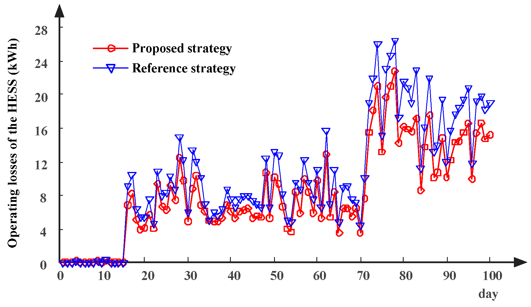
5.3. Operating Losses of the HESS

Figure 15 shows the profiles of the operating losses of the HESS when two smoothing strategies are applied to these 100 cases. The simulation results indicate that the proposed smoothing strategy has lower losses because the number of cycles of the battery is reduced.

In conclusion, the operating losses of the HESS can be reduced when using the HESS and the PV power curtailment to smooth PV power fluctuations.

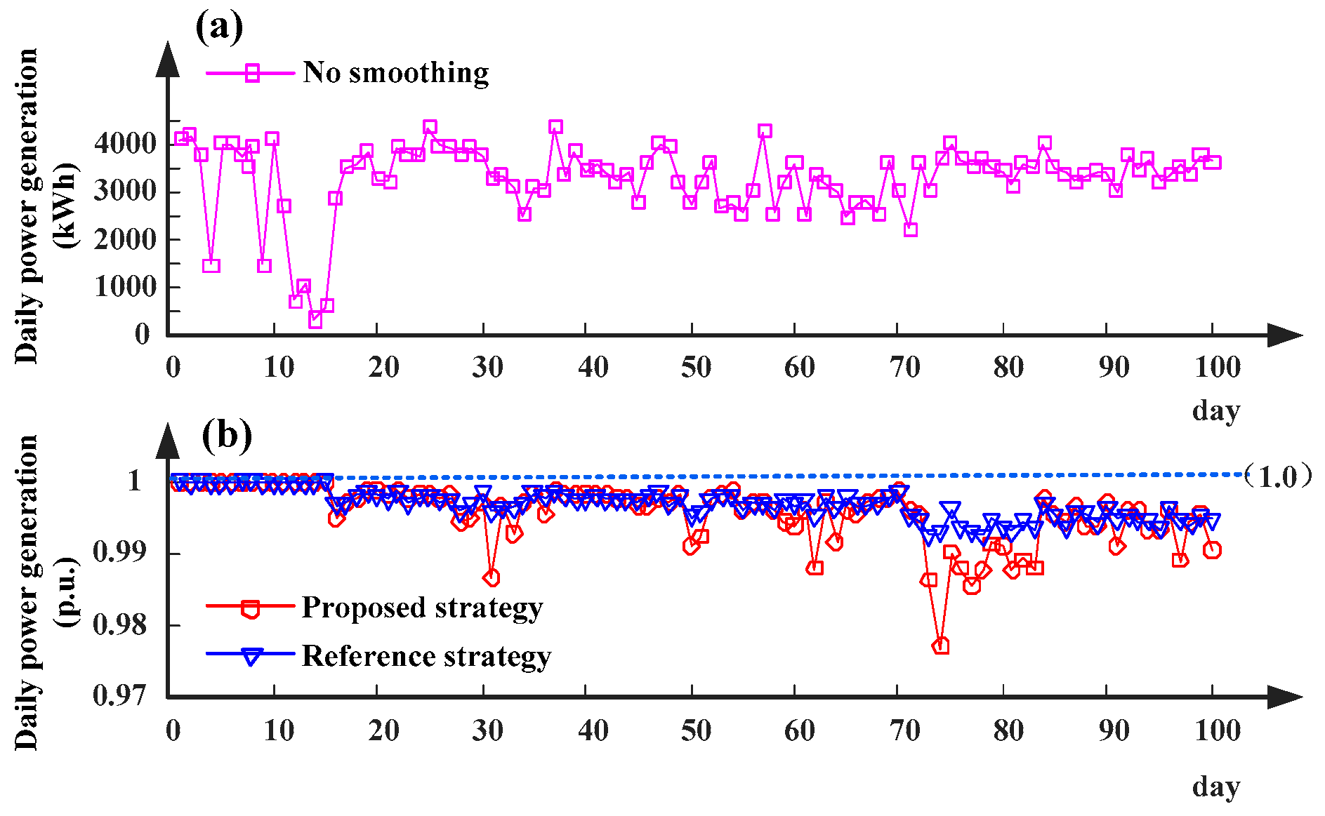
5.4. Power Generation of the PV Plant

To analyze the energy losses caused by limiting PV power, the daily power generation of these 100 cases was calculated, as shown in Figure 16. Before the suppression, the daily power generation of the PV plant is described in Figure 16a; after smoothing by the two strategies, the values of the daily power generation of the PV plant were converted into the per unit (p.u.) values for comparison, as shown in Figure 16b.

In addition, based on the power generation data obtained from these 100 cases, the annual power generation of this PV plant was estimated. If no correction action is provided, the annual power generation of this PV plant is about 325,863 kWh. The annual power generation of the reference strategy is reduced by 0.32% (324,840.81 kWh) because of the operating losses of the HESS, and the proposed strategy is reduced by 0.44% (324,424.20 kWh) because of the HESS losses and the PV power curtailment.

In conclusion, for a 750 kW PV plant, when using the HESS and the PV power curtailment to smooth PV power fluctuations, the annual power generation of the PV plant will be reduced by about 0.44%, which is slightly greater than the method of using the HESS.

5.5. Lifetime Net Profits of the PV Plant

The lifetime net profit of the PV plant is an important indicator to evaluate the economics of the different smoothing strategies. Therefore, this paper established a lifetime net profit model, which is shown as follows:

$$R_{\mathrm{NP}}(y)={\displaystyle \sum _{i=1}^y\frac{R_{\mathrm{pv}}(i)-C_{\mathrm{om}}(i)-C_{\mathrm{re}}(i)-C_{\mathrm{fine}}(i)}{{(1+r)}^{i-1}}}-C_{\mathrm{inv}}$$

(22)

where R_NP(y) represents the cumulative net profits of the PV plant in the y^th year (y ≤ 25); i is the index of the year (i ≤ y); R_pv, C_om, C_re, and C_fine represent the revenue of selling PV electricity, the operation and maintenance costs of the energy storage system, the replacement costs of the energy storage system, and the fine caused by the power fluctuations that exceed the allowable limits, respectively; C_inv is the initial investment costs of the PV plant and energy storage systems; r is the discount rate, r = 2% [27]. R_pv, C_om, C_re, C_fine, and C_inv are calculated as follows:

$$R_{\mathrm{pv}}=m_1{E}_{\mathrm{PG}}$$

(23)

where E_PG denotes the annual power generation of the PV plant. Referring to the report released by the US Energy Information Administration, the feed-in price of solar power, m₁, is set to US$0.13/kWh [28].

$$C_{\mathrm{inv}}=m_2{E}_{\mathrm{BES}}+m_3{E}_{\mathrm{SCES}}+m_4(P_{\mathrm{BES}}+P_{\mathrm{SCES}})+m_5{C}_{\mathrm{PV}}$$

(24)

where m₂, m₃, m₄, and m₅ are the unit price of batteries, supercapacitors, energy storage converters, and PV systems, respectively.

$$C_{\mathrm{om}}=\alpha C_{\mathrm{inv}}$$

(25)

where a is a conversion factor for calculating the operation and maintenance costs of the system, in this paper, a = 0.5% [27].

$$C_{\mathrm{re}}={\lambda }_1{m}_2{E}_{\mathrm{BES}}+{\lambda }_2{m}_3{E}_{\mathrm{SCES}}$$

(26)

where λ₁ and λ₂ are 0-1 variables, when the battery’s (supercapacitor’s) cumulative cycles in the i^th year reach the upper limit, then λ₁ = 1 (λ₂ = 1), otherwise, λ₁ = 0 (λ₂ = 0).

$$C_{\mathrm{fine}}=m_6{\displaystyle \sum _{d=1}^{365}{E}_{\mathrm{over},d}}$$

(27)

where E_over,d denotes the excess energy calculated by (19) on the d^th day; m₆ is the unit price of the excess energy, this paper sets m₆ = 10m₁ (i.e., US$1.3/kWh). Moreover, the other parameters of the lifetime net profit model are shown in

Table 3. Parameters of the lifetime net profit model.

Parameters	Symbols	Values	Main References
Unit price of the battery	m2	570 ($/kWh)	[29]
Unit price of the supercapacitor	m3	5800 ($/kWh)	[24]
Unit price of the energy storage converter	m4	105 ($/kWh)	[30]
Unit price of PV systems	m5	1150 ($/kW)	[31]
Lifetime of the PV plant	y	25 (years)	[24,27]
Lifetime of the battery	--	10 (years) and 3000 (cycles)	[19,24]
Lifetime of the supercapacitor	--	10 (years) and 50000 (cycles)	[19,24]

.

Overall, Figure 17 shows the profiles of the lifetime net profits of the PV plant when the two smoothing strategies are applied. As can be seen from Figure 17, the simulation results demonstrate that the proposed smoothing strategy is more economical than the reference strategy.

In conclusion, combining the HESS and the PV power curtailment is a more economical method of smoothing PV power fluctuations compared to the method of using the HESS, although it will result in more energy losses due to the PV power curtailment.

6. Conclusions

In this study, a coordinated control strategy for the HESS and PV to smooth the power fluctuations of PV was developed. The main conclusions are as follows:

(1) A PV power curtailment algorithm was developed to automatically limit the power generated by the PV converter when the HESS could not fully absorb upward power fluctuations. A multi-objective optimization model of the HESS was established to minimize the total losses of the HESS and to optimize the SOC of the supercapacitor while dispatching the power demand of the HESS. To prevent the SOC of the supercapacitor from reaching the lower limit of its constraint during the period of smoothing downward power fluctuations, a simple short-term prediction model was presented to dynamically adjust the weights of the sub-objective functions. Also, the HESS SOCs may approach their lower limits due to the curtailment of PV power and energy losses. Therefore, an SOC correction strategy of the HESS was proposed to correct the SOCs of the battery and the supercapacitor, when PV power fluctuations did not exceed the allowable range. Simulation results proved the effectiveness and correctness of the proposed strategies.

(2) Compared to the method of using the HESS to smooth PV power fluctuations, the advantages of the proposed smoothing method are as follows:

• The proposed method is more economical and can increase the net profits of the PV and HESS plant.
• The proposed method can reduce not only the cycles of batteries, but also the energy losses of the HESS.
• Under the same conditions (such as the capacities of the HESS, requirements of the power fluctuations, and the installed capacity of the PV plant), the proposed method has better performances of smoothing PV power fluctuations than the method of using the HESS.

However, the disadvantage of the proposed smoothing strategy is that limiting the PV power will reduce the power generation of PV plants. For example, the annual power generation of a 750 kWp PV plant will be reduced by 0.44% (about 1439 kWh).

It is recommended that further research be undertaken in the following aspects: (1) An optimal allocation method of the HESS is needed to determine the energy and power capacities of BES and SCES; and (2) it would be interesting to examine the use of flywheel energy storage systems (FESS) [32] as an alternative to the supercapacitor in the HESS, because the advantages of the FESS are a rapid response, low hazardous waste, high power, and long-life compared to batteries.

References

1. Wang, H.; Sun, J.B.; Wang, W.J. Photovoltaic Power Forecasting Based on EEMD and a Variable-Weight Combination Forecasting Model. Sustainability 2018, 10, 2627. [Google Scholar] [CrossRef]
2. Lave, M.; Kleissl, J.; Arias-Castro, E. High-frequency irradiance fluctuations and geographic smoothing. Sol. Energy 2012, 86, 2190–2199. [Google Scholar] [CrossRef]
3. Omran, W.A.; Kazerani, M.; Salama, M.M.A. Investigation of Methods for Reduction of Power Fluctuations Generated From Large Grid-Connected Photovoltaic Systems. IEEE Trans. Energy Convers. 2011, 26, 318–327. [Google Scholar] [CrossRef]
4. Miller, W.; Liu, A.; Amin, Z.; Wagner, A. Power Quality and Rooftop-Photovoltaic Households: An Examination of Measured Data at Point of Customer Connection. Sustainability 2018, 10, 1224. [Google Scholar] [CrossRef]
5. Marcos, J.; de la Parra, I.; García, M.; Marroyo, L. Control Strategies to Smooth Short-Term Power Fluctuations in Large Photovoltaic Plants Using Battery Storage Systems. Energies 2014, 7, 6593–6619. [Google Scholar] [CrossRef] [Green Version]
6. Marcos, J.; Marroyo, L.; Lorenzo, E.; Garca, M. Smoothing of PV power fluctuations by geographical dispersion. Prog. Photovolt. 2012, 20, 226–237. [Google Scholar] [CrossRef]
7. Shivashankar, S.; Mekhilef, S.; Mokhlis, H.; Karimi, M. Mitigating methods of power fluctuation of photovoltaic (PV) sources—A review. Renew. Sustain. Energy Rev. 2016, 59, 1170–1184. [Google Scholar] [CrossRef]
8. Lappalainen, K.; Valkealahti, S. Output power variation of different PV array configurations during irradiance transitions caused by moving clouds. Appl. Energy 2017, 190, 902–910. [Google Scholar] [CrossRef]
9. Sukumar, S.; Mokhlis, H.; Mekhilef, S.; Karimi, M.; Raza, S. Ramp-rate control approach based on dynamic smoothing parameter to mitigate solar PV output fluctuations. Int. J. Electr. Power Energy Syst. 2018, 96, 296–305. [Google Scholar] [CrossRef]
10. Zhao, J.; Xu, Z. Ramp-Limited Optimal Dispatch Strategy for PV-Embedded Microgrid. IEEE Trans. Power Syst. 2017, 32, 4155–4157. [Google Scholar] [CrossRef]
11. Anvari, M.; Werther, B.; Lohmann, G.; Wächter, M.; Peinke, J.; Beck, H.P. Suppressing power output fluctuations of photovoltaic power plants. Sol. Energy 2017, 157, 735–743. [Google Scholar] [CrossRef]
12. Li, X.; Hui, D.; Lai, X. Battery Energy Storage Station (BESS)-Based Smoothing Control of Photovoltaic (PV) and Wind Power Generation Fluctuations. IEEE Trans. Sustain. Energy 2013, 4, 464–473. [Google Scholar] [CrossRef]
13. de la Parra, I.; Marcos, J.; García, M.; Marroyo, L. Improvement of a control strategy for PV power ramp-rate limitation using the inverters: Reduction of the associated energy losses. Sol. Energy 2016, 127, 262–268. [Google Scholar] [CrossRef]
14. Das, C.K.; Bass, O.; Kothapalli, G.; Mahmoud, T.S.; Habibi, D. Overview of energy storage systems in distribution networks: Placement, sizing, operation, and power quality. Renew. Sustain. Energy Rev. 2018, 91, 1205–1230. [Google Scholar] [CrossRef]
15. Jiang, W.; Zhang, L.; Zhao, H.; Hu, R.; Huang, H. Research on power sharing strategy of hybrid energy storage system in photovoltaic power station based on multi-objective optimisation. IET Renew. Power Gener. 2016, 10, 575–583. [Google Scholar] [CrossRef]
16. Jie, W.; Ming, D. Wind power fluctuation smoothing strategy of hybrid energy storage system using self-adaptive wavelet packet decomposition. Autom. Electr. Power Syst. 2017, 41, 7–12. [Google Scholar] [CrossRef]
17. Liu, F.; Duan, S.; Liu, F.; Liu, B.; Kang, Y. A variable step size INC MPPT method for PV systems. IEEE Trans. Ind. Electron. 2008, 55, 2622–2628. [Google Scholar] [CrossRef]
18. Parra, D.; Swierczynski, M.; Stroe, D.I.; Norman, S.A.; Abdon, A.; Worlitschek, J.; O’Doherty, T.; Rodrigues, L.; Gillott, M.; Zhang, X.; et al. An interdisciplinary review of energy storage for communities: Challenges and perspectives. Renew. Sustain. Energy Rev. 2017, 79, 730–749. [Google Scholar] [CrossRef] [Green Version]
19. Evans, A.; Strezov, V.; Evans, T.J. Assessment of utility energy storage options for increased renewable energy penetration. Renew. Sustain. Energy Rev. 2012, 16, 4141–4147. [Google Scholar] [CrossRef]
20. Wang, L.; Sharkh, S.; Chipperfield, A.; Cruden, A. Dispatch of Vehicle-to-Grid Battery Storage Using an Analytic Hierarchy Process. IEEE Trans. Veh. Technol. 2017, 66, 2952–2965. [Google Scholar] [CrossRef]
21. IBM. CPLEX Optimizer. Available online: https://www.ibm.com/analytics/cplex-optimizer (accessed on 6 December 2018).
22. Hou, P.; Hu, W.H.; Zhang, B.H.; Soltani, M.; Chen, C.; Chen, Z. Optimised power dispatch strategy for offshore wind farms. IET Renew. Power Gener. 2016, 10, 399–409. [Google Scholar] [CrossRef]
23. Lai, C.S.; Jia, Y.; McCulloch, M.D.; Xu, Z. Daily Clearness Index Profiles Cluster Analysis for Photovoltaic System. IEEE Trans. Ind. Inform. 2017, 13, 2322–2332. [Google Scholar] [CrossRef]
24. Jacob, A.S.; Banerjee, R.; Ghosh, P.C. Sizing of hybrid energy storage system for a PV based microgrid through design space approach. Appl. Energy 2018, 212, 640–653. [Google Scholar] [CrossRef]
25. He, G.; Chen, Q.; Kang, C.; Xia, Q.; Poolla, K. Cooperation of Wind Power and Battery Storage to Provide Frequency Regulation in Power Markets. IEEE Trans. Power Syst. 2017, 32, 3559–3568. [Google Scholar] [CrossRef]
26. Correa-Florez, C.A.; Gerossier, A.; Michiorri, A.; Kariniotakis, G. Stochastic operation of home energy management systems including battery cycling. Appl. Energy 2018, 225, 1205–1218. [Google Scholar] [CrossRef] [Green Version]
27. Zhang, Y.; Campana, P.E.; Lundblad, A.; Yan, J. Comparative study of hydrogen storage and battery storage in grid connected photovoltaic system: Storage sizing and rule-based operation. Appl. Energy 2017, 201, 397–411. [Google Scholar] [CrossRef]
28. U.S. Energy Information Administration. Electric Power Monthly. Available online: https://www.eia.gov/electricity/monthly/index.php (accessed on 6 December 2018).
29. IRENA. Electricity Storage and Renewables: Costs and Markets to 2030. Available online: http://www.irena.org/publications/2017/%20Oct/Electricity-storage-and-renewables-costs-and-markets (accessed on 6 December 2018).
30. IRENA. The Power to Change: Solar and Wind Cost Reduction Potential to 2025. Available online: http://www.irena.org/publications%20/2016/Jun/The-Power-to-Change-Solar-and-Wind-Cost-Reduction-Potential-to-2025 (accessed on 6 December 2018).
31. IRENA. Renewable Power Generation Costs in 2017. Available online: http://www.irena.org/publications/2018/Jan/Renewable-power-generation-costs-in-2017 (accessed on 6 December 2018).
32. Mukoyama, S.; Nakao, K.; Sakamoto, H.; Matsuoka, T.; Nagashima, K.; Ogata, M.; Yamashita, T.; Miyazaki, Y.; Miyazaki, K.; Maeda, T.; et al. Development of Superconducting Magnetic Bearing for 300 kW Flywheel Energy Storage System. IEEE Trans. Appl. Supercond. 2017, 27. [Google Scholar] [CrossRef]
Figure 1. System structures of a grid-connected PV `plant with an HESS.
Sustainability 11 01324 g001
Figure 2. PV power fluctuations in one minute.
Sustainability 11 01324 g002
Figure 3. Coordinated control strategy for the HESS and PV to smooth PV power fluctuations.
Sustainability 11 01324 g003
Figure 4. Schematic diagram of the PV power curtailment algorithm.
Sustainability 11 01324 g004
Figure 5. A short-term prediction model is used to predict the energy demand of the HESS.
Sustainability 11 01324 g005
Figure 6. Typical scenarios of PV power fluctuations: (a) Scenario I; (b) scenario II; and (c) scenario III.
Sustainability 11 01324 g006
Figure 7. Active power profiles of the PV plant and the HESS: (a) the power injected into the grid before and after the suppression; (b) the curves from 12:00 to 14:00 in (a) are enlarged; (c) the profile of the overall power of the HESS; (d) the curve from 12:00 to 14:00 in (c) is enlarged; (e) the profiles of the power generated by the PV converter; and (f) the curves from 12:00 to 14:00 in (e) are enlarged.
Sustainability 11 01324 g007
Figure 8. Power fluctuation profiles before and after the suppression.
Sustainability 11 01324 g008
Figure 9. Power and SOC profiles of the HESS: (a) power of BES; (b) SOC of BES; (c) power of SCES; and (d) SOC of SCES.
Sustainability 11 01324 g009
Figure 10. Power fluctuation profiles before and after the suppression when the PV power curtailment algorithm was not applied.
Sustainability 11 01324 g010
Figure 11. Power fluctuation profiles before and after the suppression when the SOC correction strategy of the HESS was not applied.
Sustainability 11 01324 g011
Figure 12. SOC profiles of BES and SCES when the SOC correction strategy of the HESS was not applied: (a) SOC curves of BES; and (b) SOC curves of SCES.
Sustainability 11 01324 g012
Figure 13. Daily excess energy (Eover) profiles of the two smoothing strategies in 100 cases.
Sustainability 11 01324 g013
Figure 14. The profiles of nbat,eq and ncap,eq when two smoothing strategies are applied to these 100 cases: (a) the number of cycles of the battery, nbat,eq; and (b) the number of cycles of the supercapacitor, ncap,eq.
Sustainability 11 01324 g014
Figure 15. Profiles of the operating losses of the HESS when two smoothing strategies are applied to these 100 cases.
Sustainability 11 01324 g015
Figure 16. Profiles of the power generation of the PV plant when two smoothing strategies are applied to these 100 cases: (a) the daily power generation of the PV plant before the suppression; and (b) the daily power generation of the PV plant (p.u.) under different smoothing strategies.
Sustainability 11 01324 g016
Figure 17. Profiles of the lifetime net profits of the PV plant when different smoothing strategies are applied.
Sustainability 11 01324 g017