Building Asset Value Mapping in Support of Flood Risk Assessments: A Case Study of Shanghai, China


1
State Key Laboratory of Earth Surface Processes and Resource Ecology, Faculty of Geographical Science, Beijing Normal University, Beijing 100875, China
2
Key Laboratory of Environmental Change and Natural Disaster, MOE, Faculty of Geographical Science, Beijing Normal University, Beijing 100875, China
3
Department of Water & Climate Risk, Institute for Environmental Studies, Vrije Universiteit Amsterdam, De Boelelaan 1085, 1081 HV Amsterdam, The Netherlands
*
Author to whom correspondence should be addressed.
Sustainability 2019, 11(4), 971; https://doi.org/10.3390/su11040971
Submission received: 9 January 2019
/
Revised: 7 February 2019
/
Accepted: 11 February 2019
/
Published: 14 February 2019
(This article belongs to the Section Sustainability in Geographic Science)
Abstract
:Exposure is an integral part of any natural disaster risk assessment, and damage to buildings is one of the most important consequence of flood disasters. As such, estimates of the building stock and the values at risk can assist in flood risk management, including determining the damage extent and severity. Unfortunately, little information about building asset value, and especially its spatial distributions, is readily available in most countries. This is certainly true in China, given that the statistical data on building floor area (BFA) is collected by administrative entities (i.e. census level). To bridge the gap between census-level BFA data and geo-coded building asset value data, this article introduces a method for building asset value mapping, using Shanghai as an example. This method consists of a census-level BFA disaggregation (downscaling) by means of a building footprint map extracted from high-resolution remote sensing data, combined with LandScan population density grid data and a financial appraisal of building asset values. Validation with statistical data and field survey data confirms that the method can produce good results, but largely constrained by the resolution of the population density grid used. However, compared with other models with no disaggregation in flood exposure assessment that involves Shanghai, the building asset value mapping method used in this study has a comparative advantage, and it will provide a quick way to produce a building asset value map for regional flood risk assessments. We argue that a sound flood risk assessment should be based on a high-resolution—individual building-based—building asset value map because of the high spatial heterogeneity of flood hazards.
1. Introduction
Flood risk is a combination of hazard (i.e., the probability of occurrence), exposure (i.e., the elements at risk) and vulnerability (i.e., the susceptibility of those elements to damage) [1,2,3]. Exposure can be defined as the depreciated or replacement value of the tangible physical assets in hazard-prone areas [3,4]. Flood risk under climate change and socioeconomic change is a great challenge for flood risk management [5,6,7,8,9,10].
Many recent studies have focused on various types of floods in risk analysis. Paprotny and Terefenko [11], for instance, used a topographic objects database to estimate the potential impacts of sea-level rise and coastal floods in Poland. Considering flood frequency, inundation depth, and depth-damage functions, Oubennaceur and colleagues [12] assessed the expected annual damage to each individual building due to river flooding in a reach of the Richelieu River, Quebec, Canada. Röthlisberger and colleagues [13] compared five building value models for flood risk analysis, and proposed that estimating exposed-building values should be based on individual buildings rather than on areas of land-use types. Higher quality exposure data is needed to perform validations of flood risk models [14].
However, for flood risk analysis, quite often a spatial mismatch exists between hazard intensity data (e.g., inundation depth), which are frequently modelled on a high-resolution raster level, and exposure data, which are usually only available at coarse census units (e.g., counties) or aggregated land-use/land cover classes [14,15,16,17]. Flood risk assessments often invest much more in hazard modelling of water depths or inundation areas at a spatially explicit raster level [18,19], while only a limited number of studies have explicitly focused on the estimations of assets and their disaggregation to overcome the spatial mismatch between the quality of hazard and exposure data [20,21,22,23]. Meanwhile, the quality of the exposure data is one of the most important uncertainties in flood risk assessments [24,25,26,27]. Because of the high spatial resolution of water inundation depth estimation, which is mainly a function of topography [28,29], flood risk assessments are much more sensitive to the exposure data resolution than are other natural disasters, such as earthquake risk assessments [15,16].
The most consistently reliable exposure data are usually available at the administrative unit level. Previous studies have used various disaggregation methods using ancillary data to generate exposure data sets for natural disaster risk assessment, rather than simply assuming an equal spatial distribution of assets over the whole administrative area, particularly focussing on mapping of population density [21]. Several ancillary data sets have been used for building asset disaggregation. Dutta et al. [21] used gridded land cover data to disaggregate building exposure data that was estimated at a ward-level. The building floor area (BFA) per grid cell was determined using land cover types, the percentage of area covered by buildings in a given area, and the ratio of the gross BFA divided by the ground area of the buildings. The latter two parameters were usually unavailable in census data. Seifert et al. [30] used land-use data and building density fraction information to disaggregate assets into different economic sectors. By comparing three different disaggregation methods and two land-use datasets in the framework of flood damage estimation, Wünsch et al. [31] concluded that investing in land-use data quality could be better than in more sophisticated mapping techniques. Population distribution is also a widely-used proxy variable for disaggregating the building asset values from the census area to a finer resolution [32]. Thieken et al. [16] assumed that the population distribution directly reflected the distribution of residential asset values, as they found a direct correlation between the two, and therefore, they used population distribution data and land cover data as ancillary variables. Silva et al. [33] used the LandScan population distribution to disaggregate the building stock at the parish level for a disaster risk assessment in mainland Portugal. Figueiredo and Martina [17] directly used open building data, including building footprint and height, to disaggregate census data to a gridded residential BFA data set. However, a limitation of many of these previous studies is that exposure model validation is rarely performed, largely due to data scarcity for most existing study areas.
Quantification of exposed asset value is directly related the flood damage estimation. Building asset value (for fixed assets) depends on various factors, including building structure, age, and use type, but also varies in time and space [18,19].
Present methods use several approaches to estimate monetary asset values. First, land use/land cover data are used as exposure indicators, and their associated maximum damage values are given for flood damage modelling [34]. Second, asset value is estimated on an administrative unit level [30,31,32,33,34,35,36] or census block [37], then disaggregated into grid cells with the help of ancillary data, such as road networks, nightlight data, or land cover data [20,30,32]. Third, construction costs or replacement costs per square meter for different building types are used for building asset value estimation. For example, with combined standardized building construction costs with census building stock data, and by using dasymetric mapping techniques, a building asset value map was generated in Germany for natural disaster risk assessment [16,35]. However, data availability is an important factor that affects whether these methods or parameters can be used in China.
For China, statistical gross BFA data is available at the county level in the population census tabulation. BFA refers to the total floor area (measured in square meters) inside the building envelope, including the external walls and excluding the roof, and it represents the most consistent and reliable source of information about buildings. Moreover, the availability of actual building information is increasing. As each province in China contributes to building the Map World platform under the instruction of the National Administration of Surveying, Mapping and Geoinformation, they are providing electronic maps with building footprints that are generated from high-resolution remote sensing data. Both the census statistical BFA data and the building footprint data have enabled the production of a geo-coded building asset value map for reducing the uncertainty of the risk model.
In this study, we developed a method to map the building asset value using Shanghai as a case study. To test the reliability of the disaggregated BFA map, validation is performed with both statistical data and actual sampled BFA data obtained by field surveys. The remainder of the paper is structured as follows. Section 2 presents the materials and methods that are used to obtain the building asset value map. Section 3 presents the results and tests the performance of the produced BFA map, and Section 4 provides a discussion of the application of building asset value maps in flood damage modelling and the limitations in this study. Finally, Section 5 presents the conclusions.
2. Materials and Methods
2.1. Study Area
Shanghai is a low-lying coastal city situated on the eastern fringe of the Yangtze River Delta in eastern China (Figure 1). This city has the most developed economy and the highest population density in China. In 2015, Shanghai’s gross domestic product exceeded 2.5 trillion Chinese Yuan (CNY, 402.6 billion USD), and its total population surpassed 24 million inhabitants, with a population density of 3809 persons per km2. Shanghai has been impacted by sea level rise, cyclones, and storm surges [38]; this city is currently experiencing significant land-subsidence at a maximum rate of 24.12 mm/a because of massive construction [38], which in turn trends to amplify flood risk. Overall, due to its unique geographic location and a higher exposure to risk, Shanghai is considered to be one of the most vulnerable cities to coastal flooding worldwide [39,40], Shanghai’s flood risk is receiving increased media coverage and policy attention [38,39,40,41,42,43,44].
2.2. Data
This study uses three types of data (Table 1). First, the census data of Shanghai, including district-level and township-level total population data, the district-level total BFA data subdivided by both height class and building use type (Table 2), and the completed construction floor area and its cost of construction by building use type in 2014 (Table 3), are obtained from the Shanghai Municipal Statistics Bureau [45,46]. As shown in Table 2, the total population of Shanghai surpassed 24 million inhabitants in 2014. The gross BFA of Shanghai reached 1153 km2, and 53% of this BFA corresponded to residential buildings. Among the building height classes (Table 4), buildings with 1–7 storeys (low-rise buildings) represent 68% of the total BFA, buildings with 8–19 storeys (medium-rise buildings) represent 21%, and only 11% of the BFA corresponds to buildings with more than 20 storeys (high-rise buildings). Second, vector data, including a building footprint map of Shanghai, which provides information on building location and area, are obtained from the Map World of Shanghai (www.shanghai-map.net). This data is generated from high-resolution remote sensing data by the Shanghai Municipal Institute of Surveying and Mapping for 2013 and 2014. In contrast, actual building height data in the downtown area, which provide information on building height, area, and location, are acquired by field surveying with the help of aerial images. Third, raster data, including LandScan population density grids (30 arc seconds) in 2010 are developed by the Oak Ridge National Laboratory [47,48] (as shown in Figure 2).
2.3. Method
Disaggregation of the gross BFA from administrative districts to regular grid cells is the key to producing a building asset value map for Shanghai, and it can be accomplished in two main steps (Figure 3): (1) township-level BFA estimation and (2) disaggregation (or downscaling) of the gross BFA from township to regular grid cell by ancillary data (i.e., building footprint map and LandScan population density grid). The BFA disaggregation performance is evaluated in the second step through the comparison of the modelled BFA and the statistical BFA: (1) in each district for three building height classes and (2) at the grid cell level in the downtown area. Finally, building asset value can be calculated using current construction cost parameters by building use type. All these steps combined allows us to produce the building asset value map.
2.3.1. Township-Level BFA Estimation
SMSB [45] provide data on the gross BFA for each district (Table 2), but this data is not publicly available on the township level for Shanghai. Fortunately, township-level population census data are available from the Tabulation on the 2010 population census of Shanghai Municipality [46]. The township-level population was adjusted to 2014 levels according to the population growth rate of Shanghai from 2010 to 2014 (i.e., 5.34%), assuming that that the per-capita BFA is the same within a district (As the average land area for the 17 districts of Shanghai is only 373 square kilometers [45], the spatial heterogeneity of the per-capita BFA is not obvious, although it shows differences in larger districts, such as Pudong and Chongming). Then, the township-level gross BFA (BFAtownship) can be estimated by:
where is the total population of a township, and and are the census gross BFA and statistical total population of the district that the township belongs to, respectively.
2.3.2. Disaggregation of BFA from the Township to the Regular Grid Cell
As can be seen in Figure 1, the building footprint map underestimates the actual building distribution. High-rise building footprints are missing on the Map World of Shanghai (www.shanghai-map.net), mostly due to data updating frequency. This underestimation is, undoubtedly, one of the sources of uncertainty for the BFA downscaling, but these are, to our knowledge, the best available building distribution data for Shanghai.
Although the building footprint map contains the building locations, other information, such as building height class (or number of storeys), use type, and material type are not known. Hence, deriving a building-by-building asset value map in a deterministic way is not practicable. Another alternative is to develop a grid-based building asset value map, as done in this study. However, due to the fact that the gross BFA by both height class and by building use type are only known at the resolution of the administrative unit (Table 2), the disaggregation results may be no longer meaningful, which will be further discussed in Section 4.
The first step in the disaggregation of the BFA is to find a proxy for the relative BFA density distribution within a township. While population density is usually closely related with the BFA [49,50,51], the Pearson correlation value for this relationship reached 0.99 for the 17 districts of Shanghai in 2014. As such, we use LandScan population density (i.e., LandScan 2010) as a proxy for the relative BFA density distribution within a township to disaggregate BFA from the township to the regular grid cell. This implies that we assume that the BFA density distribution is proportional to the population density distribution within a township, which is a typical approach in disaggregation [52].
It is noted that the resolution of the LandScan 2010 is only approximately 800 m × 800 m in Shanghai, which is a lower resolution than the vector building footprint map. For the purpose of both facilitating the disaggregation and maintaining the high resolution of building geographic information, we transform the building footprint map from vector to raster format using 2.5 m × 2.5 m pixels and we uniformly put the LandScan population of each grid (800 m × 800 m) to the building occupied grid (2.5 m × 2.5 m) that is located under the LandScan population grid. Obviously, the newly generated population density map (2.5 m × 2.5 m) by this homogeneous distribution may be inconsistent with the actual population density distribution; for example, population density may be underestimated in high-rise buildings and overestimated in low-rise buildings. Finally, grid cell-level BFA (BFAgrid) and the derived building height (Hgrid) within a township can be calculated by:
where and are the newly generated population density value in the grid cell and the aggregated population of the township from the newly generated population density grid, respectively (Here, we use a relatively population density within a township—as ancillary indicator—to estimate the grid-cell level BFA. Because the 2014 LandScan population density grid was not available, we assume that the relative population density is the same between 2010 and 2014, which will underestimate the BFA in the new constructed area from 2010 to 2014), respectively, and is the area of the grid cell (e.g., 2.5 m × 2.5 m).
2.3.3. Evaluation of the Performance of the BFA Disaggregation Model
To evaluate the performance of the developed exposure model, we adopt two methods to validate the disaggregated BFA density map of Shanghai. First, as shown in Equation (3), for each grid cell, the building height can be derived by dividing the disaggregated BFA by the area of the occupied grid cell, then, the disaggregated gross BFA by building height class (i.e., low-rise building, medium-rise building and high-rise building) for each district can be aggregated according to the correspondence between height classes and height intervals (Table 4) gathered through a field survey of approximately 100 buildings in Shanghai. Finally, the differences between the disaggregated BFA and the real statistical BFA (Table 2) in different height classes can be identified. For the second method, information about the building height and building footprint is gathered or updated in the downtown area to validate the BFA disaggregation performance at the grid cell level. Based on the modelled BFA (BFAgrid) and the actual BFA (BFAactual) in the downtown area, the relative error of the modelled BFA (Rerror) in a grid can be calculated by:
Furthermore, we test the performances of our approach compared to other spatial interpolation methods in exposure assessment of a hypothetical flood event.
2.3.4. Valuation of Building Assets
In the research field of disaster loss estimation, there is an important distinction between methods for the valuation of assets at risk. Researchers either use replacement costs or depreciated values within their loss calculation methods [53,54,55]. The replacement cost can be interpreted as the cost of rebuilding a property exactly as it was prior to the disaster, regardless of any depreciation due to its age. This approach provides valuable information on potential pay-outs and is therefore interesting from an insurance perspective [24]. The depreciated value can be interpreted as the remaining property value, corrected for its depreciation by age [36], and it is often assumed to be the true cost that is with the loss of the asset [55]. It is important to note that the depreciation value is lower than the replacement value. Given that flood insurance is still not well developed in China, especially in rural areas, governmental financial support usually guarantees the post-disaster reconstruction of an inhabitant’s house, moreover, the latest building code is usually adopted in post-disaster reconstruction, and the newly constructed buildings are usually safer than the old ones. As such, this paper uses the current construction cost (excluding the cost of land per square meter) to produce a building asset value map for Shanghai. Overall, the construction cost value should be equal to or greater than the replacement cost value because the former adopts the higher standards of the newer building code. This evaluation may have practical implications for the government in terms of disaster risk management (i.e., financing demand in post-disaster reconstruction).
Because the individual costs per building are impossible to obtain in Shanghai, a weighted average of the construction cost by district is used for the building asset value evaluation. First, the average construction cost per square meter by building (use) type for Shanghai as a whole is calculated by dividing the cost of construction of buildings completed by the BFA completed (Table 3). Then, based on the percentage of gross BFA by building use type (residential, office, commercial, and other) in each district (Table 2), the average construction cost per square meter by district can be calculated via a weighted average method (as shown in the last column in Table 2). Finally, the building asset value in each grid cell can be estimated by multiplying the BFA (BFAgrid) by the average construction cost per square meter of the district that the grid belongs to.
3. Results
3.1. Building Asset Value Map
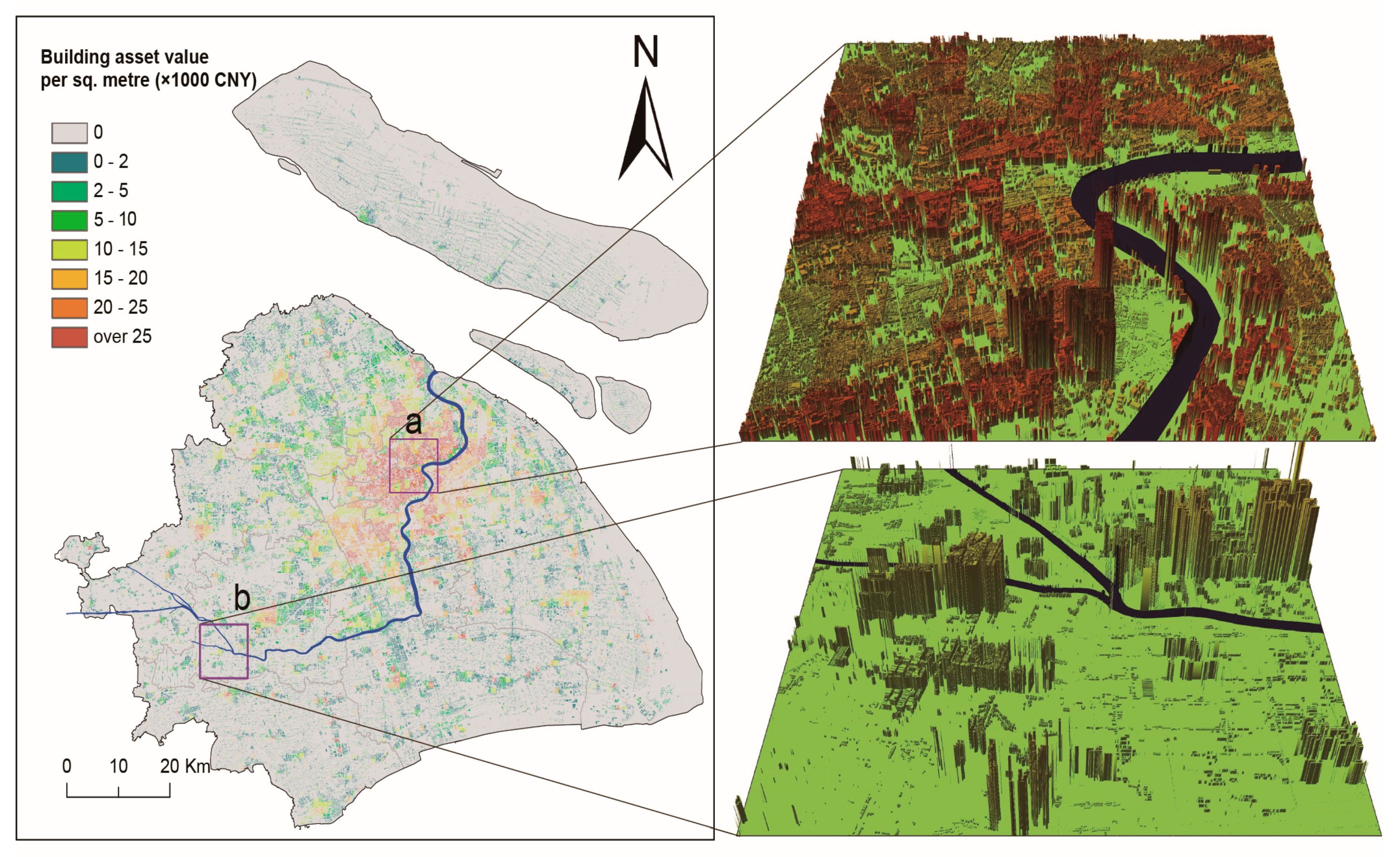
Based on the statistical data for both the district-level BFA (Table 2) and township-level population, the township-level BFA can be estimated under the assumption that the per-capita BFA is the same within a district (Equation (1)). The township-level BFA ratio can be calculated (as shown in Figure 4) by dividing the BFA by the total area of each township. As expected, the BFA ratio in the downtown area is greater than that in the surrounding area (Figure 4). More specifically, the average relative building heights are greater in Huangpu, Xuhui, Jingan, Putuo, Zhabei, and Hongkou than those in the sub-urban areas of Shanghai. By combining the township-level BFA estimation with the newly generated population density grid, the grid cell-level BFA and building height can be derived (by disaggregation) via Equations (2) and (3), respectively, and a BFA density map can be obtained. Then, by combining the average construction cost per square meter (in Table 2) and the BFA density map, the building asset value map can be produced (Figure 5); the map obtained here demonstrated that the total building asset value reached 5113.9 billion CNY (approximately USD 832.5 billion) for Shanghai in 2014.
3.2. Performance Evaluation of the Disaggregated BFA Map
On the macro level, as Figure 6 shows, there is a significant relationship between the derived BFA and the census statistical BFA disaggregated by three building height classes at the district level, the Pearson correlation coefficient reached 0.93. This figure also shows that most of the district’s medium-rise BFA is slightly overestimated, whereas both the low-rise and high-rise BFA values are slightly underestimated for most districts.
Two reasons can explain the performance of the disaggregated BFA grid on a macro level. First, the coarse resolution of the LandScan population density data used is one the main reasons. This coarse resolution smooths out the high- and low- population density areas in the new generated population density grid used as ancillary indicator for the BFA disaggregation, which is likely the main reason that underlies the overestimation of the medium-rise BFA in most districts in Shanghai. Moreover, as the population density is not fully correlated with the BFA, such as in the villa residential and ‘village in the city’ layouts of some Chinese cities.
To further validate the accuracy of the modelled (or disaggregated) BFA at the sub-district level, we compare the modelled BFA with the actual BFA (acquired by field surveys) grid-by-grid in the downtown area of Shanghai. As Figure 7 shows, the actual building height information of the downtown area of Shanghai (Figure 7a) is transformed into the number of building storeys by the relationship between the building height and the number of storeys (Figure 7b and Table 4) and, subsequently, into a BFA density map. Comparing the disaggregated BFA map (Figure 7d) with the actual BFA map (Figure 7c) reveals that, based on visual judgement, both underestimations and overestimations of the BFA occur in the downtown area; for example, the BFA is underestimated in the eastern side of the downtown area (as shown by the black circle in Figure 7d). Overall, the modelled BFA underestimated 6.1% of the actual BFA for the downtown area as a whole.
Furthermore, compared with the actual BFA distribution grid-by-grid in the downtown area, the variance of relative error of the modelled BFA decreases as the grid resolution decreases (Figure 7e). For example, when the regular grid resolution is 800 m × 800 m, the relative error of the modelled BFA (compared with the actual BFA density distribution) is mainly distributed in the range [−1, 1]. This variance is lower than that for the grid resolution of 100 m × 100 m (i.e., [−1, 3]). The modelled BFA is significantly correlated with the actual BFA at the 1600 m grid cell size level (Figure 7f), and the spatial distribution of the relative error is presented in Figure 7g.
In summary, the BFA disaggregation precision is affected by the spatial mismatch between the coarse resolution ancillary data (e.g., population density grid) and the high-resolution building location data. The actual spatial resolution of the modelled BFA map should be lower than the resolution of the LandScan population density grid (i.e., 800 m × 800 m), as a population density within an 800 m × 800 m grid cell is meaningless.
3.3. Comparison of Different Exposure Models on Flood Exposure Assessment
Because the reliability of the BFA distribution is the key for building asset value mapping, we estimate the affected BFA for a hypothetical flood event in the downtown area of Shanghai, using different exposure models.
We use a flood scenario event generated by Ke [56], who modelled a flood with a 1/10,000 per year probability of water levels along Huangpu River in Shanghai, assuming no flood protection (Figure 8). Because the flood protection project in the Huangpu River in Shanghai has a return period of one in two hundred years [57], it may be assumed that weak riverine segments will always fail under a probability of the 1/10,000 per year flood. Moreover, flood hazards can be characterized by high river flows, with resulting inundations and also inundation duration [58]. If using a multivariate joint probability distribution for the return period analysis of floods, an extreme flood event based only on water level (univariate variable) for the return period analysis by Ke [56] may be downgraded when considering both the water level and the water volume in a joint probability analysis [59,60,61]. For similar examples, a 1 in 200 per year extreme high water event will change into a 1 in 75 per year joint probability level when considering both an extreme high-water event and significant wave height [61], while an 81-year return period dust storm based on dust storm duration (univariate variable) will change into a 4-year joint return period dust storm, based on both the dust storm duration and the maximum wind speed, with the help of Copula-based approach [62]. Overall, as flood hazard modelling is outside of the scope of this study, we simply use an extreme flooding scenario to demonstrate how the disaggregated exposure map could be overlaid with the hazard intensity in flood exposure assessment.
Although the maximum inundation depths in Shanghai are lower than 2.5 m for a flooding event characterized by a 10,000-year return period (Figure 8), and only the ground-floors (first floor) of buildings are directly affected by flooding, indirect flood effects may be induced, even though the building levels above the ground floor are not directly damaged [63]. For example, reduced housing service value may be incurred by flood-induced business limitations or disruptions, there may be disadvantages connected with reduced market and public services, and there might even be long-term building damage due to soaking or subsistence [63,64]. As such, flood exposure is defined in a broader sense in this study—that being the building stock that is located within the inundation extent, and not restricted to building assets that are directly affected (i.e., the ground floor of buildings) [58].
As shown in Table 5, for a flood scenario in the downtown area of Shanghai, disaggregation of BFA is significantly affected by flood exposure estimation. First, no disaggregation leads to a greater underestimation of flood exposure than that of the proposed model by this study, because the BFA density is greater in the downtown area than that in the rural area. It can be predicted that the flood exposure estimation will be overestimated in the rural area under the assumption of the uniform spatial distribution of BFA within a district. Second, using the township-level population to adjust the BFA distribution within a district is an important step to improve the accuracy of the exposure model. By this adjustment, the relative error decreases from 36%, with no disaggregation (BFA uniformly distributed within district), to 8% for the flood exposure estimation. Meanwhile, the adjustment of the BFA from non-building occupied areas to building-occupied areas by using building footprint data with no disaggregation (BFA uniformly distributed in building-occupied areas within a district) only reduces the relative error of the estimated flood exposure by 5%. This is mainly due to the fact that the non-building-occupied areas are very limited in the crowded downtown area of Shanghai.
4. Discussion
4.1. Application of the Building Asset Value Map in Scenario-Based Flood Damage Modelling
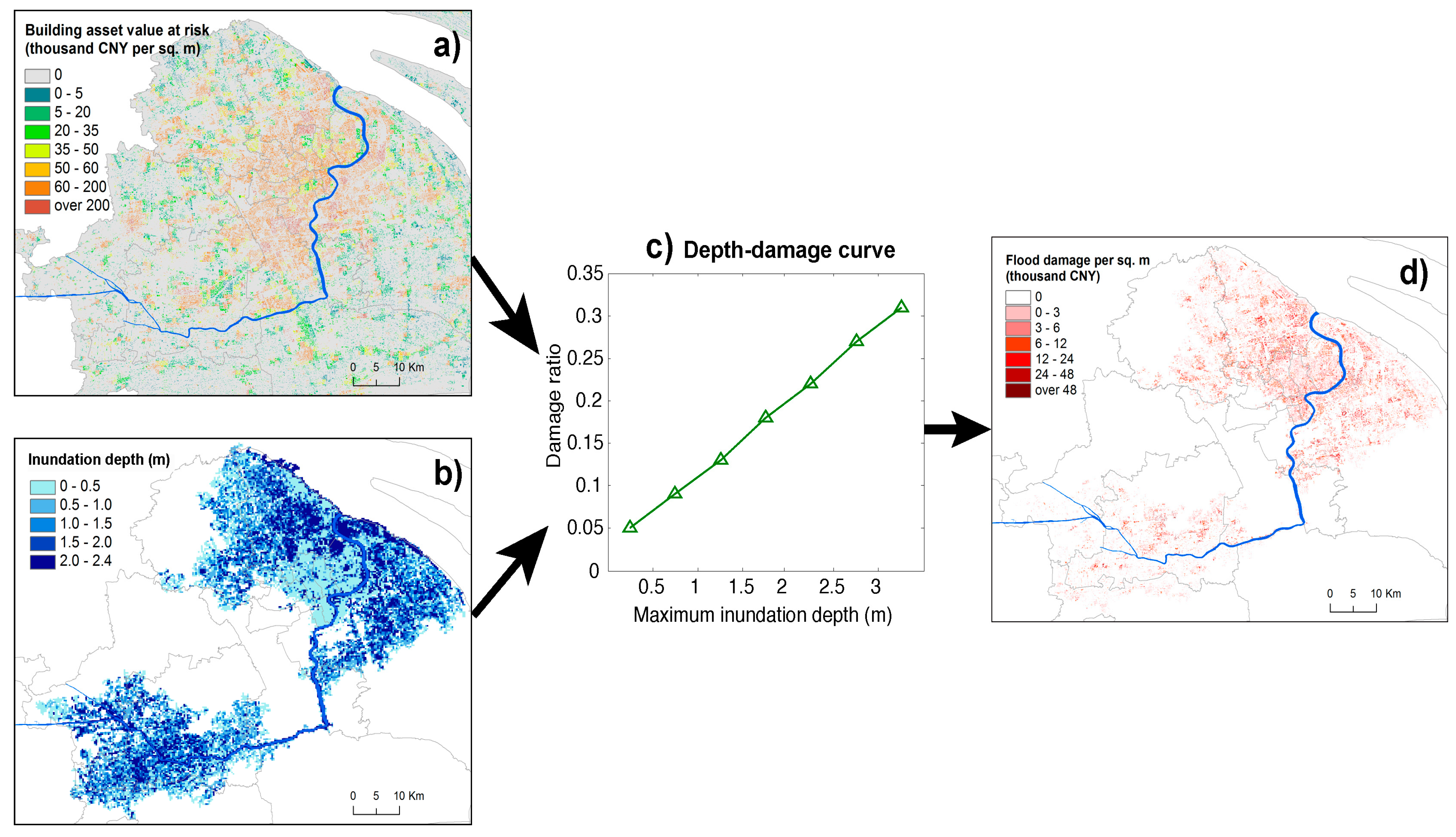
The most commonly used method for assessing flood losses is a combination of depth-damage curves, an exposure map, and an inundation map. By using these depth-damage curves, information on inundation and the spatial distribution of people and assets can be combined to assess the damage for any given cell on the exposure map, based on the depth in the inundation map [65]. Figure 9 shows the application diagram of the building asset value map that is used in flood loss modelling.
Both the flood inundation map (Figure 9b) for a flood with a 1/10,000 per year probability for the Huangpu River as described above, and the depth-damage curves (Figure 9c) were from Ke [56]. The depth-damage curve is recognized as the primary source of uncertainty in flood damage estimation [26]; thus, here, we only use the depth-damage curve for commercial buildings (Figure 9c) as a simple example for modelling flood damage.
In reality, however, for the building asset values at risk of flooding, only a small proportion of the building will be exposed to the flood. This is especially the case for high-rise buildings. Green [66] identified a relationship between population density and the ratio of net assets exposed to flooding, and recommended that one-sixth of the assets should be considered as the exposed value when the population density is above 15,000/km2, one-quarter when the population density is between 8000/km2 and 15,000/km2, half when the population density is between 1000/km2 and 8000/km2, and 1 when the population density is less than 1000/km2 [66]. Based on this assumption, we use the LandScan population density and the building asset value map generated by this study to determine the exposed building asset value.
Finally, we can determine that the exposed building asset value reached 1868.3 billion CNY (approximately USD 304.1 billion) by an overlay analysis of Figure 9a,b; this value corresponds to 36.5% of the total building asset value of Shanghai. Combined with the depth-damage curve (Figure 9c), the total direct economic damage for buildings can be calculated as the sum of the damages in all inundated grid cells (Figure 9d), which results in approximately 197.6 billion CNY (USD 32.2 billion) of damage for this flood scenario.
It should be noted, however, that the flooding scenario we use in this application to produce estimates of economic losses is far from realistic. For example, this hypothetical scenario did not consider flood protection in Shanghai, while in reality, the flood protection project in the Huangpu River in Shanghai has a return period of one to two hundred years; hence, the simulated flood damage should be overestimated. As flood risk modelling is outside of the scope of this study, we simply use an extreme flooding scenario to demonstrate how the disaggregated building asset value map can be overlaid with the hazard intensity in flood risk assessments.
4.2. Limitations
The application of the method presented in Section 2.3 makes it possible to create a grid-based building asset exposure map for flood risk assessment with a certain level of resolution, since this method consists of using actual geo-referenced building footprints maps and statistical BFA census data. However, because the input data are limited, the maximum resolution of the gridded building asset value map is also limited.
First, the building footprint map provides the locations and footprints of all of the buildings in Shanghai, but other information, including building height, building use type, material type, year of construction, and construction cost, is only available at the resolution of the administrative unit. Therefore, the distribution of this information is retained, regardless of the grid cell size, when performing the spatial downscaling of census data.
Second, to produce a more realistic building asset value map, this paper resorted to using LandScan population density data to derive the BFA density distribution information under the assumption that the per-capita BFA is the same within a township; as such, the disaggregated BFA is only valid up to a certain level of grid spatial resolution, which largely corresponds to the limit of the representativeness of the LandScan population density grid (800 m × 800 m) that is used to represent the BFA density distributions. Moreover, although we display the BFA map at a resolution of 2.5 m × 2.5 m (to retain the actual building location information), at higher resolutions, (i.e., when the grid cell size is smaller than 800 m × 800 m), the BFA distributions for each regular cell are meaningless. Meanwhile, using the average density distribution of the BFA within a grid cell size of 800 m × 800 m corresponding to the population density will cause smoothing of the building height, resulting in the underestimation of both the high-rise and low-rise BFA values in most districts (as shown in Figure 6). Using high-resolution remote sensing data (LiDAR data) to extract building height and urban structure [67,68] should avoid the use of the 2010 LandScan population density grid, this data is just a yearly average of population density, and gaps exist for the actual BFA distribution.
Finally, a weighted (by building use type) average construction cost per square meter at district-level resolution was used in the building asset value evaluation, and thus, the spatial differences in the construction cost (by building use type) were neglected. More detailed information about both the distribution of building use types and the spatial variability of the construction costs would be useful for further improving the building asset value estimation, as shown above. However, the optimal building asset value estimation model depends on this requirement within the context of flood risk management, and estimating building asset values based on individual buildings should be better than on areas of land use types [13].
5. Conclusions
Uncertainties in the value of exposed assets is known to be one of the major drivers of uncertainties in quantitative flood risk analyses. Given the existence of a mismatch between high spatial resolution hazard modelling and coarse exposure data in flood risk assessment, this paper proposes a method to disaggregate census building floor area to the regular grid cell level by using ancillary data, and then transforms this into a building asset value map via the construction cost per square meter of BFA. The building asset map obtained using this method was shown to identify the spatial distribution and density of building asset with reasonable resolution, but it is constrained by the resolution of the input data, including: (1) the ancillary data used, including the coarse resolution of population density grid, (2) the incomplete nature of publicly available building information, and in particular, their number of storeys as well as the building use types. The flood exposure estimation under a flood scenario, obtained by applying different exposure models demonstrated that the disaggregation method proposed by this study is a powerful tool for improving the accuracy of the estimation of flood exposure in terms of affected BFA when compared to models based on the assumption of a uniform distribution of the BFA within an administrative unit. The advantage of the disaggregation method developed in this paper is that building asset value maps can be quickly produced if three main datasets are available: a building footprint map, a population density map, and census statistical BFA data. The building asset value maps produced represent a good alternative for exposure analysis in flood risk assessment.
It should be emphasized that the provincial Map World platform, under the instruction of the National Administration of Surveying, Mapping and Geoinformation of China, has been working on obtaining spatial data for buildings, including information on the number of storeys; for example, in the downtown areas for some developed cities. Such up-to-date information, including building footprints, and building structure types and ages, will allow for the accurate estimation of not only the building floor area at the grid cell level, but also the replacement cost. When these data become available, it will be possible to generate an exposure dataset on a building on the basis of the building, rather than by land-use types, which will improve the data quality for building asset exposure for natural disaster risk estimation.
There remains a question of how high the asset exposure resolution should be, in order to conduct satisfactory flood risk modelling. Compared to the resolution and detail of flood hazard modelling, even the most detailed asset assessments are regarded as coarse [18], since physical asset values are very heterogeneous in space and time, including building assets. Ideally, acquiring actual building-by-building information (e.g., location, footprint, height, and structure type) could satisfy the demand for exposure data input for flood risk analysis. This approach is feasible for small or medium sized areas, but not for huge areas, where the process would be too time-consuming and costly. To summarize, we believe that the details required for building asset value mapping depend strongly on the size of the study area, the available input data, and the required accuracy of the flood risk assessment. We argue that because of the high spatial heterogeneity of flood hazards, a sound flood risk assessment should be based on a high-resolution asset value map—individual building-based asset value map—as focused upon by this study.
Author Contributions
J.W. and E.K. conceived and designed the study; X.W., J.W. and M.Y. analyzed the data; J.W. and M.Y. wrote the paper; J.W., M.Y. and E.K. revised the manuscript.
Funding
This study was financially supported by the National Key Research and Development Program, grant number 2016YFA0602403, and the National Natural Science Foundation of China, grant umber 41571492.
Acknowledgments
The authors are grateful to Qian Ke for providing the flood hazard scenario data for Shanghai. The authors are also grateful to the two anonymous reviewers for their very valuable comments on an earlier version of this manuscript.
Conflicts of Interest
The authors declare no conflict of interest.
References
- Ward, P.J.; Jongman, B.; Aerts, J.C.J.H.; Bates, P.D.; Botzen, W.J.W.; Diaz Loaiza, A.; Hallegatte, S.; Kind, J.M.; Kwadijk, J.; Scussolini, P.; et al. A global framework for future costs and benefits of river–flood protection in urban areas. Nat. Clim. Chang. 2017, 7, 642–646. [Google Scholar] [CrossRef]
- Jevrejeva, S.; Jackson, L.P.; Grinsted, A.; Lincke, D.; Marzeion, B. Flood damage costs under the sea level rise with warming of 1.5 °C and 2 °C. Environ. Res. Lett. 2018, 13. [Google Scholar] [CrossRef]
- Amadio, M.; Mysiak, J.; Carrera, L.; Koks, E.E. Improving flood damage assessment models in Italy. Nat. Hazards 2016, 82, 2075–2088. [Google Scholar] [CrossRef] [Green Version]
- Ye, M.; Wu, J.; Wang, C.; He, X. Historical and Future Changes in Asset Value and GDP in Areas Exposed to Tropical Cyclones in China. Wea. Clim. Soc. 2019, 11, 307–319. [Google Scholar] [CrossRef]
- Koks, E. Moving flood risk modelling forwards. Nat. Clim. Chang. 2018, 8, 561–562. [Google Scholar] [CrossRef]
- Molinari, D.; Scorzini, A.R. On the Influence of Input Data Quality to Flood Damage Estimation: The Performance of the INSYDE Model. Water 2017, 9, 688. [Google Scholar] [CrossRef]
- Li, W.; Wen, J.; Xu, B.; Li, X.; Du, S. Integrated Assessment of Economic Losses in Manufacturing Industry in Shanghai Metropolitan Area Under an Extreme Storm Flood Scenario. Sustainability 2019, 11, 126. [Google Scholar] [CrossRef]
- Fang, Y.; Du, S.; Scussolini, P.; Wen, J.; He, C.; Huang, Q.; Gao, J. Rapid Population Growth in Chinese Floodplains from 1990 to 2015. Int. J. Environ. Res. Public Health 2018, 15, 1602. [Google Scholar] [CrossRef]
- Rana, I.A.; Routray, J.K. Multidimensional Model for Vulnerability Assessment of Urban Flooding: An Empirical Study in Pakistan. Int. J. Disaster Risk Sci. 2018, 9, 359–375. [Google Scholar] [CrossRef]
- Du, S.; He, C.; Huang, Q.; Shi, P. How did the urban land in floodplains distribute and expand in China from 1992–2015? Environ. Res. Lett. 2018, 13, 034018. [Google Scholar] [CrossRef] [Green Version]
- Paprotny, D.; Terefenko, P. New estimates of potential impacts of sea level rise and coastal floods in Poland. Nat. Hazards 2017, 85, 1249–1277. [Google Scholar] [CrossRef]
- Oubennaceur, K.; Chokmani, K.; Nastev, M.; Lhissou, R.; El Alem, A. Flood risk mapping for direct damage to residential buildings in Quebec, Canada. Int. J. Disaster Risk Reduct. 2019, 33, 44–54. [Google Scholar] [CrossRef]
- Röthlisberger, V.; Zischg, A.P.; Keiler, M. A comparison of building value models for flood risk analysis. Nat. Hazards Earth Syst. Sci. 2018, 18, 2431–2453. [Google Scholar] [CrossRef]
- Molinari, D.; De Bruijn, K.M.; Castillo–Rodríguez, J.T.; Aronica, G.T.; Bouwer, L.M. Validation of flood risk models: Current practice and possible improvements. Int. J. Dis. Risk Reduct. 2019, 33, 441–448. [Google Scholar] [CrossRef]
- Chen, K.; McAneney, J.; Blong, R.; Leigh, R.; Hunter, L.; Magill, C. Defining area at risk and its effect in catastrophe loss estimation: A dasymetric mapping approach. Appl. Geogr. 2004, 24, 97–117. [Google Scholar] [CrossRef]
- Thieken, A.; Müller, M.; Kleist, L.; Seifert, I.; Borst, D.; Werner, U. Regionalisation of asset values for risk analyses. Nat. Hazards Earth Syst. Sci. 2006, 6, 167–178. [Google Scholar] [CrossRef] [Green Version]
- Figueiredo, R.; Martina, M. Using open building data in the development of exposure data sets for catastrophe risk modelling. Nat. Hazards Earth Syst. Sci. 2016, 16, 417–429. [Google Scholar] [CrossRef] [Green Version]
- Merz, B.; Kreibich, H.; Schwarze, R.; Thieken, A. Review article ‘Assessment of economic flood damage’. Nat. Hazards Earth Syst. Sci. 2010, 10, 1697–1724. [Google Scholar] [CrossRef]
- Chinh, D.T.; Dung, N.V.; Gain, A.K.; Kreibich, H. Flood Loss Models and Risk Analysis for Private Households in Can Tho City, Vietnam. Water 2017, 9, 313. [Google Scholar] [CrossRef]
- Gunasekera, R.; Ishizawa, O.; Aubrecht, C.; Blankespoor, B.; Murray, S.; Pomonis, A.; Daniell, J.E. Developing an adaptive global exposure model to support the generation of country disaster risk profiles. Earth–Sci. Rev. 2015, 150, 594–608. [Google Scholar] [CrossRef]
- Dutta, D.; Herath, S.; Musiake, K. A mathematical model for flood loss estimation. J. Hydrol. 2003, 277, 24–49. [Google Scholar] [CrossRef]
- Merz, B.; Kreibich, H.; Thieken, A.; Schmidtke, R. Estimation uncertainty of direct monetary flood damage to buildings. Nat. Hazards Earth Syst. Sci. 2004, 4, 153–163. [Google Scholar] [CrossRef] [Green Version]
- Amadio, M.; Mysiak, J.; Marzi, S. Mapping Socioeconomic Exposure for Flood Risk Assessment in Italy. Risk Anal. 2018. [Google Scholar] [CrossRef] [PubMed]
- Jongman, B.; Kreibich, H.; Apel, H.; Barredo, J.I.; Bates, P.D.; Feyen, L.; Gericke, A.; Neal, J.; Aerts, J.C.J.H.; Ward, P.J. Comparative flood damage model assessment: towards a European approach. Nat. Hazards Earth Syst. Sci. 2012, 12, 3733–3752. [Google Scholar] [CrossRef] [Green Version]
- De Moel, H.; Aerts, J.C.J.H. Effect of uncertainty in land use, damage models and inundation depth on flood damage estimates. Nat. Hazards 2011, 58, 407–425. [Google Scholar] [CrossRef]
- De Moel, H.; Bouwer, L.M.; Aerts, J.C.J.H. Uncertainty and sensitivity of flood risk calculations for a dike ring in the south of the Netherlands. Sci. Total Environ 2014, 473–474, 224–234. [Google Scholar] [CrossRef] [PubMed]
- Meyer, V.; Becker, N.; Markantonis, V.; Schwarze, R.; van den Bergh, J.C.J.M.; Bouwer, L.M.; Bubeck, P.; Ciavola, P.; Genovese, E.; Green, C.; et al. Review article: Assessing the costs of natural hazards–State of the art and knowledge gaps. Nat. Hazards Earth Syst. Sci. 2013, 13, 1351–1373. [Google Scholar] [CrossRef]
- Apel, H.; Martìnez Trepat, O.; Hung, N.N.; Chinh, D.T.; Merz, B.; Dung, N.V. Combined fluvial and pluvial urban flood hazard analysis: concept development and application to Can Tho city, Mekong Delta, Vietnam. Nat. Hazards Earth Syst. Sci. 2016, 16, 941–961. [Google Scholar] [CrossRef]
- Viero, D.P.; Peruzzo, P.; Carniello, L.; Defina, A. Integrated mathematical modeling of hydrological and hydrodynamic response to rainfall events in rural lowland catchments. Water Resour. Res. 2016, 50, 5941–5957. [Google Scholar] [CrossRef]
- Seifert, I.; Thieken, A.H.; Merz, M.; Borst, D.; Werner, U. Estimation of industrial and commercial asset values for hazard risk assessment. Nat. Hazards 2010, 52, 453–479. [Google Scholar] [CrossRef]
- Wünsch, A.; Herrmann, U.; Kreibich, H.; Thieken, A.H. The Role of Disaggregation of Asset Values in Flood Loss Estimation: A Comparison of Different Modeling Approaches at the Mulde River, Germany. Environ. Manag. 2009, 44, 524–541. [Google Scholar] [CrossRef] [PubMed] [Green Version]
- Wu, J.; Li, Y.; Li, N.; Shi, P. Development of an Asset Value Map for Disaster Risk Assessment in China by Spatial Disaggregation Using Ancillary Remote Sensing Data. Risk Anal. 2018, 38, 17–30. [Google Scholar] [CrossRef] [PubMed]
- Silva, V.; Crowley, H.; Varum, H.; Pinho, R. Seismic risk assessment for mainland Portugal. Bull. Earthq. Eng. 2014, 13, 429–457. [Google Scholar] [CrossRef]
- De Moel, H.; van Vliet, M.; Aerts, J.C.J.H. Evaluating the effect of flood damage–reducing measures: A case study of the unembanked area of Rotterdam, the Netherlands. Reg. Environ. Chang. 2014, 14, 895–908. [Google Scholar] [CrossRef]
- Kleist, L.; Thieken, A.H.; Köhler, P.; Müller, M.; Seifert, I.; Borst, D.; Werner, U. Estimation of the regional stock of residential buildings as a basis for a comparative risk assessment in Germany. Nat. Hazards Earth Syst. Sci. 2006, 6, 541–552. [Google Scholar] [CrossRef]
- Wu, J.; Li, N.; Shi, P. Benchmark wealth capital stock estimations across China’s 344 prefectures: 1978 to 2012. China Econ. Rev. 2014, 31, 288–302. [Google Scholar] [CrossRef]
- FEMA (Federal Emergency Management Agency). HAZUS: Multi–Hazard Loss Estimation Model Methodology—Flood Model; FEMA: Washington, DC, USA, 2003.
- Wang, J.; Gao, W.; Xu, S.Y.; Yu, L.Z. Evaluation of the combined risk of sea level rise, land subsidence, and storm surges on the coastal areas of Shanghai, China. Clim. Chang. 2012, 115, 537–558. [Google Scholar] [CrossRef]
- Hallegatte, S.; Green, C.; Nicholls, R.J.; Corfee–Morlot, J. Future flood losses in major coastal cities. Nat. Clim. Chang. 2013, 3, 802–806. [Google Scholar] [CrossRef]
- Balica, S.F.; Wright, N.G.; van der Meulen, F. A flood vulnerability index for coastal cities and its use in assessing climate change impacts. Nat. Hazards 2012, 64, 73–105. [Google Scholar] [CrossRef] [Green Version]
- Du, S.; Gu, H.; Wen, J.; Chen, K.; Van Rompaey, A. Detecting Flood Variations in Shanghai over 1949–2009 with Mann–Kendall Tests and a Newspaper–Based Database. Water 2015, 7, 1808–1824. [Google Scholar] [CrossRef]
- Wang, C.; Du, S.; Wen, J.; Zhang, M.; Gu, H.; Shi, Y.; Xu, H. Analyzing explanatory factors of urban pluvial floods in Shanghai using geographically weighted regression. Stoch. Environ. Res. Risk Assess. 2017, 31, 1777–1790. [Google Scholar] [CrossRef]
- Yin, J.; Yu, D.; Yin, Z.; Wang, J.; Xu, S. Modelling the anthropogenic impacts on fluvial flood risks in a coastal mega–city: a scenario–based case study in Shanghai, China. Landsc. Urban Plan. 2015, 136, 144–155. [Google Scholar] [CrossRef]
- Scholten, N. Flood Risk in Shanghai: Economic Impact and Adaptation Options; VU Amsterdam: Amsterdam, The Netherlands, 2016. [Google Scholar]
- SMSB (Shanghai Municipal Statistics Bureau). Shanghai Statistical Yearbook 2015; China Statistics Press: Beijing, China, 2015.
- SMSB. Tabulation on the 2010 Population Census of Shanghai Municipality; China Statistics Press: Beijing, China, 2012.
- Bhaduri, B.; Bright, E.; Coleman, P.; Dobson, J. LandScan: Locating people is what matters. Geoinformatics 2002, 5, 34–37. [Google Scholar]
- Dobson, J.E.; Bright, E.A.; Coleman, P.R.; Durfee, R.C.; Worley, B.A. LandScan: A global population database for estimating populations at risk. Photogramm. Eng. Remote Sens. 2000, 66, 849–858. [Google Scholar]
- Gallup, J.L.; Mellinger, A.D.; Sachs, J.D. Geography and economic development. Int. Reg. Sci. Rev. 1999, 22, 179–232. [Google Scholar] [CrossRef]
- Felkner, J.; Townsend, R. The Geographic Concentration of Enterprise in Developing Countries. Q. J. Econ. 2011, 126, 2005–2061. [Google Scholar] [CrossRef] [PubMed] [Green Version]
- Naroll, R. Floor Area and Settlement Population. Am. Antiq. 1962, 27, 587–589. [Google Scholar] [CrossRef]
- Aubrecht, C.; Steinnocher, K.; Köstl, M.; Züger, J.; Loibl, W. Long–term spatio–temporal social vulnerability variation considering health–related climate change parameters particularly affecting elderly. Nat. Hazards 2013, 68, 1371–1384. [Google Scholar] [CrossRef]
- Blong, R. A new damage index. Nat. Hazards 2003, 30, 1–23. [Google Scholar] [CrossRef]
- Kreibich, H.; Seifert, I.; Merz, B.; Thieken, A.H. Development of FLEMOcs—A new model for the estimation of flood losses in companies. Hydrol. Sci. J. 2010, 55, 1302–1314. [Google Scholar] [CrossRef]
- Penning–Rowsell, E.; Viavattene, C.; Pardoe, J.; Chatterton, J.; Parker, D.; Morris, J. The Benefits of Flood and Coastal Risk Management: A Handbook of Assessment Techniques; Flood Hazard Research Centre: Middlesex, UK, 2010. [Google Scholar]
- Ke, Q. Flood Risk Analysis for Metropolitan Areas—A Case Study for Shanghai; Delft Academic Press: Delft, The Netherlands, 2014. [Google Scholar]
- Research group of Control and Countermeasure of flood. Control and Countermeasure of Flood in China. China Flood Drought Manag. 2014, 24, 46–48. [Google Scholar] [CrossRef]
- Merz, B.; Hall, J.; Disse, M.; Schumann, A. Fluvial flood risk management in a changing world. Nat. Hazards Earth Syst. Sci. 2010, 10, 509–527. [Google Scholar] [CrossRef] [Green Version]
- Prime, T.; Brown, J.M.; Plater, A.J. Flood inundation uncertainty: the case of a 0.5% annual probability flood event. Environ. Sci. Policy 2016, 59, 1–9. [Google Scholar] [CrossRef]
- Brunner, M.I.; Seibert, J.; Favre, A.C. Bivariate return periods and their importance for flood peak and volume estimation. Wire’s Water 2016, 3, 819–833. [Google Scholar] [CrossRef] [Green Version]
- Wadey, M.P.; Brown, J.M.; Haigh, I.D.; Dolphin, T.; Wisse, P. Assessment and comparison of extreme sea levels and waves during the 2013/14 storm season in two UK coastal regions. Nat. Hazards Earth Syst. Sci. 2015, 15, 2209–2225. [Google Scholar] [CrossRef] [Green Version]
- Li, N.; Liu, X.; Xie, W.; Wu, J.; Zhang, P. The Return Period Analysis of Natural Disasters with Statistical Modeling of Bivariate Joint Probability Distribution. Risk Anal. 2013, 33, 134–145. [Google Scholar] [CrossRef]
- Sultana, Z.; Sieg, T.; Kellermann, P.; Müller, M.; Kreibich, H. Assessment of Business Interruption of Flood–Affected Companies Using Random Forests. Water 2018, 10, 1049. [Google Scholar] [CrossRef]
- Koks, E.E.; Bočkarjova, M.; de Moel, H.; Aerts, J.C.J.H. Integrated direct and indirect flood risk modeling: development and sensitivity analysis. Risk Anal. 2015, 35, 882–900. [Google Scholar] [CrossRef]
- Messner, F.; Meyer, V. Flood damage, vulnerability and risk perception—Challenges for flood damage research. In Flood Risk Management: Hazards, Vulnerability and Mitigation Measures; Springer: Berlin, Germany, 2006. [Google Scholar]
- Green, C. The Global Estimation of Losses from Coastal Flooding; Middlesex University: Middlesex, UK, 2010. [Google Scholar]
- Gerl, T.; Bochow, M.; Kreibich, H. Flood Damage Modeling on the Basis of Urban Structure Mapping Using High–Resolution Remote Sensing Data. Water 2014, 6, 2367–2393. [Google Scholar] [CrossRef]
- Schröter, K.; Lüdtke, S.; Redweik, R.; Meier, J.; Bochow, M.; Ross, L.; Nagel, C.; Kreibich, H. Flood loss estimation using 3D city models and remote sensing data. Environ. Modell. Softw. 2018, 105, 118–131. [Google Scholar] [CrossRef]
Figure 1.
Location of Shanghai and comparison of the building footprint (red polygon in a, b and c) and aerial image (from Google Earth) in three selected areas (a, b and c). The building footprints in both a and c are relatively consistent with the actual building distribution as reflected by the aerial image, both of them being located in a less-developed region with mainly low-rise buildings. For area b, the building coverage from the building footprint maps underestimated the actual building-occupied areas due to their missing the building footprints for some high-rise buildings.

Figure 2.
LandScan population density of Shanghai in 2010 (Data source: Oak Ridge National Laboratory [47,48]).

Figure 3.
Flowchart of the method.

Figure 4.
Distribution of the township-level BFA ratio in Shanghai. The township-level BFA ratio is equal to the BFA divided by the total land area for each township, and it reflects the virtual average building height in the township (i.e., the building density distribution). A BFA ratio of greater than one indicates that the BFA exceeds the total land area of the township (i.e., multiple storey buildings are dominant in this township).

Figure 5.
Distribution of the disaggregated building asset value (at current 2014 prices, grid cell: 2.5 m × 2.5 m) in Shanghai. Two regions are magnified to show the building asset value density in three dimensions.
Figure 5.
Distribution of the disaggregated building asset value (at current 2014 prices, grid cell: 2.5 m × 2.5 m) in Shanghai. Two regions are magnified to show the building asset value density in three dimensions.

Figure 6.
Relationship between the modelled BFA and the census statistical BFA in 17 districts with three buildings height classes: low-rise buildings: 1~7 storeys, medium-rise buildings: 8~19 storeys, and high-rise buildings: over 20 storeys.
Figure 6.
Relationship between the modelled BFA and the census statistical BFA in 17 districts with three buildings height classes: low-rise buildings: 1~7 storeys, medium-rise buildings: 8~19 storeys, and high-rise buildings: over 20 storeys.

Figure 7.
BFA validation grid-by-grid in the downtown area of Shanghai. (a) Actual building height in the downtown area of Shanghai (i.e., the sampling area used for validation). (b) Relationship between the building height and number of storeys in Shanghai, acquired by random building surveys. (c) Actual BFA density map, calculated according to the number of storeys via (a,b) multiplied by the area occupied by the building footprint. (d) Modelled BFA density map obtained as described above. (e) Distribution of the relative error between the modelled BFA and the actual BFA for five different grid cell sizes (e.g., the 2.5 m × 2.5 m gridded BFA map was resampled to a 100 m × 100 m grid cell map, and also for other grid cell sizes). (f) Relationship between the modelled BFA and the actual BFA for a regular grid cell size of 1600 m. (g) Spatial relative error distribution between the modelled BFA density and the actual BFA density for 120 regular grids with a cell size of 1600 m for the downtown area.

Figure 8.
A flood scenario along the Huangpu River with a 1/10,000 chance of occurrence for the indicated water levels in Shanghai (Data source: Ke [56]).
Figure 8.
A flood scenario along the Huangpu River with a 1/10,000 chance of occurrence for the indicated water levels in Shanghai (Data source: Ke [56]).

Figure 9.
Flow diagram of the flood damage modelling methodology, based on the maps of building asset value at risk (a) and inundation depth (b) and the depth-damage curve (c). Both the flood inundation map (grid cell size resampled from 300 m × 300 m to 2.5 m × 2.5 m under the scenarios of no embankment along the Huangpu River with a 1/10,000 per year chance of occurrence) and the depth-damage curve of Shanghai are from Ke [56]. (d) Spatial distribution of the simulated flood damage.


Table 1.
Data used for building asset value mapping in Shanghai.
| Data Name | Data Type | Spatial Resolution | Data Source | Data Year |
|---|---|---|---|---|
| Total population (persons) per township | Statistical data | Township level | SMSB [46] | 2010 |
| Total population (persons) per district | Statistical data | District level | SMSB [45] | 2014 |
| Total BFA (km2) with six height classes | Statistical data | District level | SMSB [45] | 2014 |
| Yearly completed construction floor area (km2) and its cost [Chinese Yuan (CNY) per m2] of construction by building use type | Statistical data | Shanghai | SMSB [45] | 2014 |
| Building footprint maps | Vector | Per building | Map World of Shanghai (www.shanghai-map.net) | 2013~2014 |
| Actual building height (m) information in downtown area | Vector | Per building | Field survey and aerial images | 2014~2015 |
| LandScan population density (persons per km2) grid | Raster | 30’’ (~800 m in Shanghai) | Oak Ridge National Laboratory [47,48] | 2010 |
Table 2.
District-level building floor area (BFA) by both height class and use type in Shanghai in 2014. The specified population is the total population for each district in 2014 (Data source: SMSB [45]).
Table 2.
District-level building floor area (BFA) by both height class and use type in Shanghai in 2014. The specified population is the total population for each district in 2014 (Data source: SMSB [45]).
| District | Population (Thousands) | Gross BFA (km2) | Gross BFA by Height Class (%) | Gross BFA by Building Use Type (%) | Average Construction Cost per sq. m (in 2014 Prices) | ||||||
|---|---|---|---|---|---|---|---|---|---|---|---|
| Residential Building | Non-Residential Building | 1~7 Storeys | 8~19 Storeys | ≥20 Storeys | Residential Building | Office Building | Commercial Building | Other | |||
| Pudong | 5451.2 | 142.9 | 121.8 | 67.6 | 22.4 | 10.0 | 54.0 | 5.6 | 6.3 | 34.2 | 4417.3 CNY (USD 719.1) |
| Huangpu | 682.0 | 17.6 | 19.6 | 39.1 | 17.3 | 43.5 | 47.3 | 19.4 | 13.9 | 19.5 | 5133.1 CNY (USD 835.6) |
| Xuhui | 1109.7 | 33.9 | 25.3 | 53.7 | 22.0 | 24.3 | 57.3 | 11.9 | 6.1 | 24.7 | 4687.3 CNY (USD 763.1) |
| Changning | 698.6 | 24.1 | 15.6 | 49.9 | 21.3 | 28.8 | 60.7 | 12.4 | 8.0 | 18.9 | 4758.4 CNY (USD 774.6) |
| Jing’an | 248.6 | 8.2 | 9.4 | 31.3 | 15.1 | 53.5 | 46.5 | 20.4 | 11.5 | 21.6 | 5124.0 CNY (USD 834.1) |
| Putuo | 1296.1 | 36.0 | 22.2 | 53.8 | 22.2 | 23.9 | 61.9 | 7.9 | 7.6 | 22.6 | 4566.5 CNY (USD 743.4) |
| Zhabei | 848.5 | 22.6 | 14.9 | 59.3 | 21.6 | 19.1 | 60.2 | 7.8 | 7.8 | 24.2 | 4557.5 CNY (USD 741.9) |
| Hongkou | 838.2 | 22.3 | 13.2 | 54.9 | 20.8 | 24.4 | 62.9 | 11.5 | 7.4 | 18.2 | 4718.5 CNY (USD 768.1) |
| Yangpu | 1323.7 | 33.8 | 23.3 | 64.8 | 24.1 | 11.1 | 59.1 | 7.2 | 4.9 | 28.8 | 4467.1 CNY (USD 727.2) |
| Minhang | 2539.5 | 75.2 | 54.2 | 68.6 | 29.5 | 2.0 | 58.1 | 2.2 | 5.0 | 34.7 | 4255.0 CNY (USD 692.7) |
| Baoshan | 2024.0 | 54.0 | 37.8 | 75.0 | 22.2 | 2.8 | 58.9 | 2.7 | 5.4 | 33.0 | 4288.3 CNY (USD 698.1) |
| Jiading | 1566.2 | 33.6 | 40.4 | 73.5 | 22.1 | 4.5 | 45.4 | 5.0 | 7.9 | 41.6 | 4394.0 CNY (USD 715.3) |
| Jinshan | 797.1 | 14.7 | 25.4 | 88.2 | 11.0 | 0.8 | 36.6 | 3.4 | 8.7 | 51.3 | 4313.8 CNY (USD 702.3) |
| Songjiang | 1755.9 | 39.5 | 49.8 | 79.5 | 18.7 | 1.9 | 44.2 | 1.9 | 5.9 | 47.9 | 4217.0 CNY (USD 686.5) |
| Qingpu | 1208.3 | 21.2 | 31.1 | 84.8 | 14.1 | 1.1 | 40.6 | 2.2 | 6.8 | 50.5 | 4232.8 CNY (USD 689.1) |
| Fengxian | 1167.6 | 21.6 | 29.2 | 84.5 | 13.1 | 2.3 | 42.5 | 2.9 | 6.9 | 47.7 | 4274.0 CNY (USD 695.8) |
| Chongming | 701.6 | 9.7 | 9.3 | 94.4 | 5.6 | 0.1 | 51.0 | 3.4 | 6.0 | 39.7 | 4302.3 CNY (USD 700.4) |
| Shanghai | 24256.8 | 610.9 | 542.5 | 68.0 | 21.1 | 10.9 | 53.0 | 5.9 | 6.7 | 34.4 | 4433.6 CNY (USD 721.8) |
Table 3.
The construction cost per square meter by building use type in 2014 in Shanghai (Data source: SMSB [45]). The construction cost per square meter is calculated by dividing the cost of construction of buildings completed by the BFA completed.
Table 3.
The construction cost per square meter by building use type in 2014 in Shanghai (Data source: SMSB [45]). The construction cost per square meter is calculated by dividing the cost of construction of buildings completed by the BFA completed.
| Building Use Type | BFA Completed (Million sq. m) | Cost of Construction of Buildings Completed (Billion CNY) | Construction Cost per m2 (in 2014 Prices) |
|---|---|---|---|
| Residential building | 15.4 | 64.4 | 4197.0 CNY (USD 683.2) |
| Office building | 1.7 | 13.4 | 8117.3 CNY (USD 1321.4) |
| Commercial building | 2.1 | 12.4 | 5933.0 CNY (USD 965.8) |
| Others | 4.0 | 15.6 | 3867.2 CNY (USD 629.6) |
Table 4.
Correspondence between height classes and height intervals from field surveys in Shanghai. (Data source: the authors).
Table 4.
Correspondence between height classes and height intervals from field surveys in Shanghai. (Data source: the authors).
| Number of Storeys | Height (h, m) |
|---|---|
| 1 | h ≤ 5.0 |
| 2 | 5.0 < h ≤ 11.0 |
| 3 | 11.0 < h ≤ 14.0 |
| 4 | 14.0 < h ≤ 16.0 |
| 5 | 16.0 < h ≤ 18.0 |
| 6 | 18.0 < h ≤ 21.0 |
| 7+ | 3.6 m per storey |
Table 5.
Estimated flood exposure in the downtown area for a flood scenario, using different exposure models.
Table 5.
Estimated flood exposure in the downtown area for a flood scenario, using different exposure models.
| Model | Affected BFA (km2) | Ratio |
|---|---|---|
| Best estimate by field survey | 253.43 | - |
| Proposed method by this study | 237.82 | 0.94 |
| No disaggregation (BFA uniformly distributed within district) | 162.02 | 0.64 |
| No disaggregation (BFA uniformly distributed in building occupied area within district) | 174.79 | 0.69 |
| Disaggregation using township population-adjusted BFA (BFA uniformly distributed within township) | 233.01 | 0.92 |
© 2019 by the authors. Licensee MDPI, Basel, Switzerland. This article is an open access article distributed under the terms and conditions of the Creative Commons Attribution (CC BY) license (http://creativecommons.org/licenses/by/4.0/).
Share and Cite
MDPI and ACS Style
Wu, J.; Ye, M.; Wang, X.; Koks, E. Building Asset Value Mapping in Support of Flood Risk Assessments: A Case Study of Shanghai, China. Sustainability 2019, 11, 971. https://doi.org/10.3390/su11040971
AMA Style
Wu J, Ye M, Wang X, Koks E. Building Asset Value Mapping in Support of Flood Risk Assessments: A Case Study of Shanghai, China. Sustainability. 2019; 11(4):971. https://doi.org/10.3390/su11040971
Chicago/Turabian StyleWu, Jidong, Mengqi Ye, Xu Wang, and Elco Koks. 2019. "Building Asset Value Mapping in Support of Flood Risk Assessments: A Case Study of Shanghai, China" Sustainability 11, no. 4: 971. https://doi.org/10.3390/su11040971
Note that from the first issue of 2016, this journal uses article numbers instead of page numbers. See further details here.