1. Introduction
Atmospheric pollution is currently one of the most important environmental problems on a global scale, with a direct and principal impact on human health [
1,
2]. For this reason, the European Environmental Agency conducted a study which concluded that large proportion of European populations and ecosystems are still exposed to air pollution that exceeds European standards, and therefore a considerable impact on human health and on the environment persists [
3].
Regulatory levels of ambient air quality referring to this particulate issue (
and
) are highlighted in Directive
of the European Parliament and of the council [
4]. The implementation of those measures is contained in the Royal Decree
on the improvement for ambient air quality of the Spanish Government [
5]. This issue defines a common strategy to define and establish objectives for ambient air quality in the community and assess the ambient air quality on the basis of common methods and criteria.
Air quality in cities is not limited to a single factor. In fact, it depends on multiple causes such as meteorological variables, topographical characteristics, the degree of industrialization, and traffic and population densities [
6,
7,
8,
9]. The problem of atmospheric pollutants and their effects on health and the environment, as well as the intrinsic complexity of these phenomena, justifies the need for developing management and control strategies that safeguard the environment. These problems have attracted the interest of environmental authorities and researchers, which have developed different air quality models as forecasting strategies.
Modeling atmospheric pollutants is a powerful analysis tool with multiple applications, e.g., the evaluation of emission control strategies, support in environmental decision making, generation of scientific information for a better understanding of the atmosphere dynamics and pollution in an area, etc. The importance of the models relies on the development and implementation of environmental policies, predictions of pollutant levels, information systems, forewarning and prevention of environmental pollution, or standardization of databases. Regarding the industrial sector, they can also report on the effects of new installations and the optimization of processes.
Mathematical models are generally used to simulate the physical and chemical processes that affect pollutants, and their dispersion and transformation in the atmosphere. As indicated before, the diffusion mechanism of the pollutants in the atmosphere is a complex process that depends on numerous parameters, making the development of traditional mathematical models more difficult.
The purpose of the study was twofold: to draw up a detailed analysis of the environmental, meteorological, and seasonal variables that may influence the levels of suspended particles in order to build a solid and reliable database, and to develop and assess regression models applied to forecast particulate matter in the Bay of Algeciras with a prediction horizon of 24 h. This area has the most complex environmental issues in Andalusia because it is located in the Straits of Gibraltar. Furthermore, the zone brings together large volumes of the population and a significant industrial and port development. For this reason, the Bay of Algeciras has an extensive network of air quality stations; this availability of data enabled us to improve, explore, and develop predictive models.
The regression models developed in this work are based on different techniques of artificial neural networks (
), multiple linear regression (
), and persistence. These models are based on statistical and empirical equations, in connection with the data relative to pollution and other variables that may influence it. Regarding the last two of them, we can highlight: persistence [
10,
11,
12,
13,
14] and
MLP [
9,
15,
16,
17,
18].
It is common knowledge that
ANN’s are applied in tasks of prediction and have been extensively used in myriad works. The approaches in References [
18,
19,
20,
21,
22,
23,
24] apply
ANN-based models, which are indexes that support the present research.
The paper is organized as follows.
Section 2 presents the region and the raw data from the on-site equipment.
Section 3 summarizes the theoretical framework. The experimental procedure is outlined in
Section 4, and the results are presented in
Section 5. Finally, our conclusions are explained in
Section 6.
2. Target Area and Experimental Data
The Bay of Algeciras is located in the south of Andalusia, Spain. It is around 10 km long by 8 km wide, covering an area of some 75 km
. The global and regional variations in the climate, along with the topographical conditions of the area studied, affect the transport and dispersion of pollutants [
25,
26,
27].
The data utilized in the simulation models came from the European Environment Agency database where the information is collected by air quality stations of the Environmental Quality Surveillance Network in Andalusia, as well as by using other methods [
28,
29]. These data are the combination of meteorological and air pollutants parameter measurements that were used as exogenous variables in the configuration of the proposed models. Time-series from the measurement stations belonging to the Bay of Algeciras for the period from 2005 to 2010 were used.
The stations are strategically located with the goal of improving the spatial distribution data of pollution in the Bay of Algeciras (Andalusia) (
Figure 1), providing a high density grid of measurement points over the region. These stations are designed to monitor the levels of air pollution in urban areas, traffic, maximum values or background contamination.
Table 1 and
Table 2 contain detailed descriptions of all of the parameters that can be monitored or displayed through these stations.
| Stations: | | |
| : -Rinconcillo | : Los Barrios | : Economato |
| : Algeciras EPS | : T.M. Palmones | : Guadarranque |
| : : El Zabal | : Cortijillos | : Puente Mayorga |
| : La Línea | : : Colegio Carteya | : Madrevieja |
| : : Los Barrios | : Estación San Roque | : T.M. Cepsa (10 m) |
| : : Alcornocales | : Campamento | : T.M. Cepsa (60 m) |
| : : Palmones | : Hostelería | : Tarifa |
| : T.M. CTLB (15 m) | | |
| Parameters: | | |
| : Sulphur dioxide | : Nitrogen oxide | : Particulate matter less than 1 m |
| : Carbon monoxide | : Ozone | : Methane |
| : Nitrogen monoxide | : Particulate matter less than 10 m | : Non-methane hydrocarbon |
| : Nitrogen dioxide | : Particulate matter less than 2.5 m | : Hydrogen sulphide |
| Parameters: | | |
| : Reduced Sulphur compounds | : Ethylbenzene | : Relative humidity |
| : Toluene | : Wind speed | : Barometric pressure |
| : Benzene | : Wind direction | : Solar radiation |
| : p-xylene | : Temperature | : Rainfall |
The pollutants and meteorological variables were selected taking into account the following criteria:
Limited data availability according to: (1) location of measurement stations, (2) measured parameters in each one, and (3) period of update of the European Environment Agency database.
Reliability of data, considering the obtained data with a higher percentage of validity.
The geographical location, selecting the stations in the principal urban areas of El Campo de Gibraltar.
Invalid data may have been caused by possible faults in the sensors of the measuring stations, poor calibration of the equipment, configuration errors, power outages, etc.
Table 3 shows the valid percentages of particulate matter
corresponding to the period between 2005 and 2010. Because a greater number of measuring stations measure
, these stations were used in the study.
The database is built with variables that are selected by regression analysis, and is complemented with success/error tests. This database contains information regarding the parameter to be predicted, concentrations of other atmospheric pollutants, meteorological variables, day of the week (DW), season (SS), and autoregressive data. Furthermore, all selected data had to satisfy a minimum of 85% of all measured annual data during three consecutive years as acceptance criterion. This minimum threshold of measures was chosen in order to obtain a database where the evolution and seasonality of the variables were registered.
From the analysis carried out and considering the main urban centers of El Campo de Gibraltar, three databases were obtained for the development of models in the municipalities of San Roque, Algeciras, and La Línea de la Concepción.
3. Prediction Models
In this work, five forecasting methodologies were used. They were classified into parametric and nonparametric. The parametric techniques consist of persistence and multiple linear regression models, while the nonparametric techniques are based on ANNs. More precisely, three ANN types were used: adaptive linear neuron, multilayer, and radial basis function.
3.1. Persistence Model
It is the most common reference method for forecasting horizons up to 3–6 h and needs no complex computation. It states that the predicted value at one time instance
t (
) is similar to the last measurement (
) [
14].
3.2. Multiple Linear Regression
The model has at least two predictors. Regression analysis conveys the idea of finding descriptive or predictive models from the observed relationships in a set of data. It is a widely used method in the prediction of atmospheric pollutants. Linear multiple regression defines the level and the dependence relationship of the involved parameters [
15].
3.3. Adaptive Linear Neuron
These networks are simpler than feedforward networks as they do not have hidden layers. The training of this model is based on the Widrow–Holf rule [
30], which obtains the weights and biases minimizing the mean square error (
MSE—Equation (
1)).
where
N is the number of data,
is the observed data, and
is the predicted data.
3.4. Multilayer Perceptron
Multilayer structure, which is based on the error backpropagation via the Levenberg–Marquardt paradigm, is the most extended method. This technique consists of updating the weights of the connections between neurons in a way that the weights are directly proportional to the estimated error between the desired output and the outputs that occur at each step of an iterative process [
31].
3.5. Radial Basis Function (RBF)
RBF networks have similar structures to that of a multilayer one [
32]. The main difference arises in the hidden neurons, and operates on the Euclidean distance between an input with respect to the synaptic vector (the so-called centroid). The localized neurons respond uniquely with an appreciable intensity when the presented input vector and the centroid of the neuron fall into a nearby area in the input space. The training of
RBF networks comprises two stages. The first is one unsupervised and accomplished by obtaining cluster centers of the training set inputs. The second consists of solving linear equations.
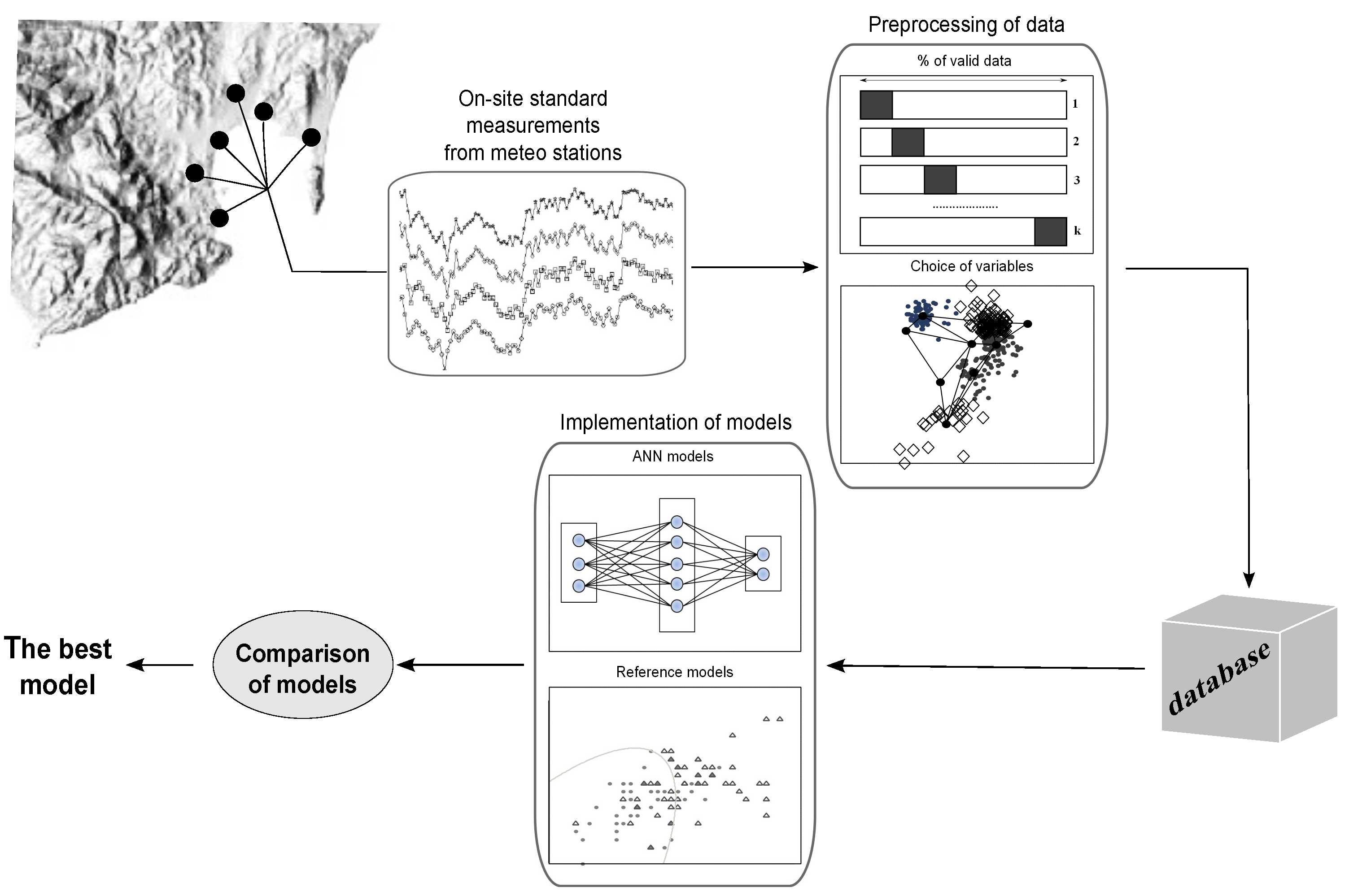
4. Experimental Procedure
The experimental procedure, depicted in the conceptual map of
Figure 2, consists of the following stages:
Data preprocessing.
Model implementation.
Model evaluation.
4.1. Preprocessing of Data
In this step, the stations that exceed 85% of valid data were selected. In addition, the statistical analysis was performed in order to eliminate the outliers. Finally, the variables of the database were ordered according to the correlation coefficient between the exogenous variables and the variable under study to be predicted ( concentration).
4.2. Implementation of the Models
The implementations of the reference models (persistence and MLR) did not present any problem.
Regarding the ANN models evaluated in this paper, they are made up of: a linear network (LIN), backpropagation network with one and two hidden layers (BP1 and BP2), and radial basis function network. The following premises are declared for all of them:
Data were normalized so that they fall into the interval [
, 1], to achieve a faster computation. Equation (
1) shows the used algorithm where
x is an element of the vector (input or output) to normalize,
is the value of the greatest element of the vector to normalize,
is the value of the smallest element of the vector to normalize,
y is the normalized value of
x,
is the maximum value (1), and
is the maximum value (
).
The dataset was randomly divided into three subsets: training, evaluation, and test sets. The first two sets were used for ANN model building with 70% and 15% of the data, respectively; and the third set, with the last 15%, was used to test the predictive power of a model using the out-of-sample set.
A total of 100 experiments were repeated for each model to avoid randomness limiting the results. Training of the tested networks was carried out until the validation error started increasing. At this point, the training was stopped, and the performance of the network was assessed.
The simulation started without exogenous variables and then we progressively added variables (from the highest to lowest correlation).
Hereinafter, the particularities of the models are detailed.
Table 4 collects parameters, corresponding to the network architecture and the activation functions for the neural networks.
The rule to select the range of the neurons in the hidden layers for
BP1 and
BP2 models is described as follows. The number of neurons in the first hidden layer is the mean of the neurons between the input and output layers, while for the second hidden layer it is one half of the neurons in the first hidden layer [
31], as shown in
Table 4.
For the RBF model, it is compulsory to specify the appropriate value of the Gaussian Kernel spread. If this value is too small or too high the network might not generalize well and a lot of neurons would be required to fit a fast-changing approximation function.
4.3. Evaluation of the Models
The models performance was assessed via the following four quality indicators: Pearson’s correlation coefficient (
), the index of agreement (IOA), the mean absolute error (
MAE), and the root mean square error (
RMSE).
where
is the covariance between
(observed data) and
(predicted data), and
and
are their respective standard deviations,
N is the number of data.
5. Results
As mentioned in
Section 2, three databases were obtained for the development of the models in the cities of San Roque, Algeciras, and La Línea de la Concepción. These databases were designed according to the correlation coefficient between the exogenous variables and the variable to be predicted, obtaining the relations shown in
Table 5. Although the inclusion of exogenous variables with correlation coefficients lower to 0,6 would appear to be a mistake, these were applied because of the large volume of data. Thanks to computing power of the models used, we were able to study the appropriateness of using such data.
After data is preprocessed, the four quality indexes of all implemented models are obtained, selecting the best configurations as a function of the number of exogenous variables. For example, the database used in San Roque has ten exogenous variables and it is designed according to the coefficient of correlation between the exogenous variables (rows 4 to 13) and the variable to be predicted (row 3), obtaining the relation shown in
Table 5.
Once the models which best minimized the errors of the evaluation set were selected, they were used to test the predictive power of a model using the out-of-sample set. The results are shown in
Table 6.
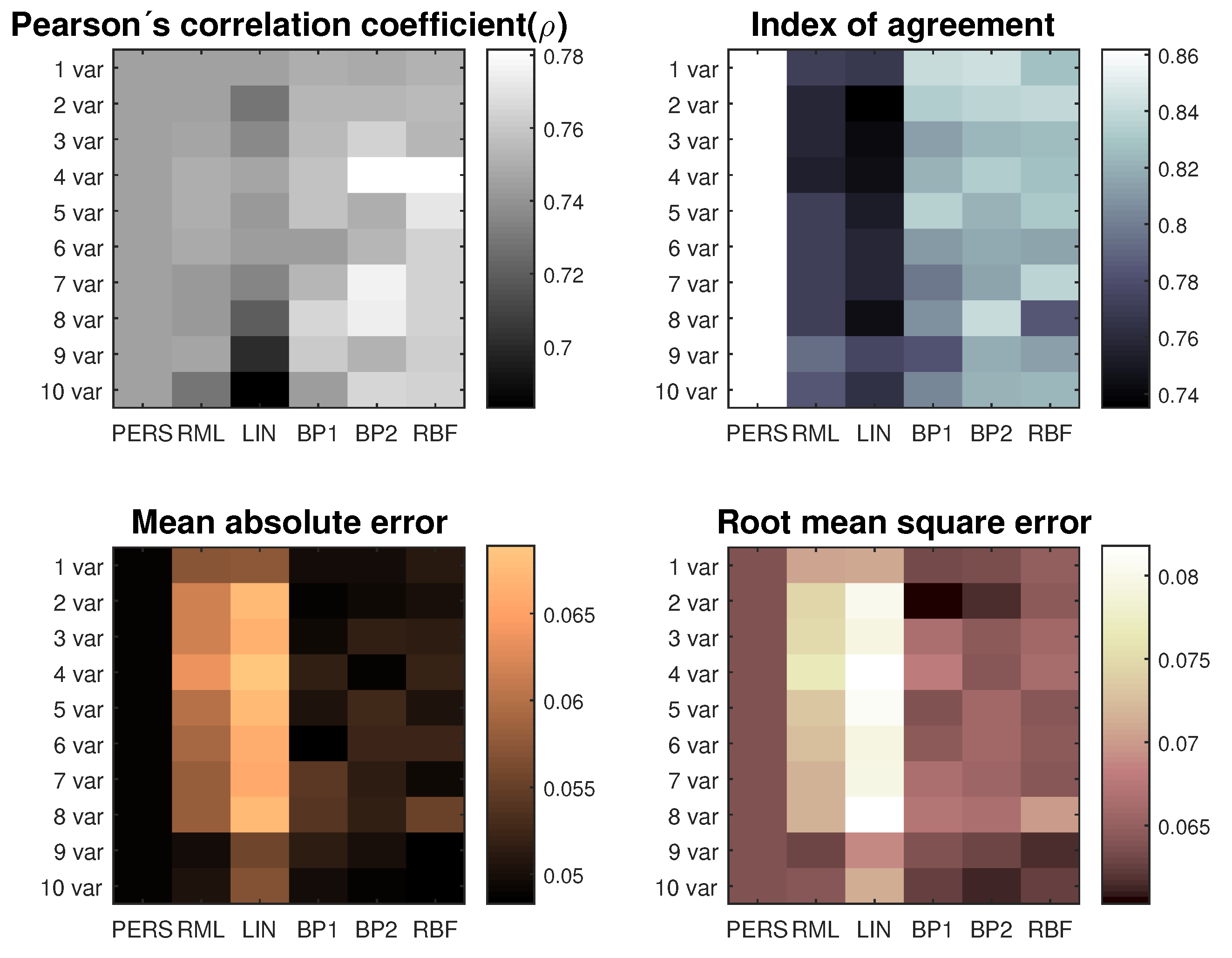
In order to select the best models, colored maps like the one depicted in
Figure 3 were used in each city area. As can be seen from the graphs, the best model within each evaluated type maximizes the values of
R and
IOA and minimizes those of
MAE and
RMSE. In the cases where it was not possible to optimize all of the indicators, only those that minimized the indicators of the errors were chosen (because the performance function that was used to build the assessed models is based on the error performance). The results obtained in each city, according to these criteria are shown in
Table 7.
After an in-depth assessment of the colored maps of each municipality and the results obtained in
Table 7, the following outcomes were concluded:
In San Roque, the BP2 model with 10 exogenous variables is the best with respect to the reference models. The optimal configuration of the BP2 model is as follows: number of neurons in the hidden layer , number of neurons in the hidden layer , training condition: and performance function: .
In Algeciras, the RBF model with 3 exogenous variables is the best with respect to the reference models. The optimal configuration of the RBF model is as follows: number of neurons in the hidden layer , spread , and performance function: .
In La Línea de la Concepción, the RBF model with 6 exogenous variables is the best with respect to the reference models. The optimal configuration of the RBF model is as follows: number of neurons in the hidden layer , spread , and performance function: .
Figure 4 shows the best obtained result for each city for daily concentration of particulate matter. These levels of concentration are standardized based on the limit value of the 150
that is the current 24 h
set by the National Ambient Air Quality Standards since 1987 [
33].
6. Conclusions
In this paper, five forecasting methodologies have been classified according to parametric and nonparametric techniques with the goal of predicting the averaged concentration of over the course of 24 h. These models were definitively used in three urban centers: San Roque, Algeciras, and La Línea de la Concepción.
Different results were obtained according to the locations under study. With respect to the reference models, the best one and their percentages of improvement as regards MAE and RMSE in each of them are as follows: San Roque (BP2 model with 10 exogenous variables; %, — and %, —), Algeciras (RBF model with 3 exogenous variables; %, — and %, —), and La Línea de la Concepción (RBF model with 6 exogenous variables; %, — and %, —).
In summary, it can be concluded that the prediction results with the proposed models exceed those obtained with the reference models. This proves that it is possible to improve performance by using additional information from the existing nonlinear relationships between the concentration of the pollutants and the meteorological variables. In this sense, the inclusion of new stations from other nets of meteorological stations and/or amateur observers available on websites should be used to increase the data sources [
34], thus improving the performance of the models . By contrast, the main drawback of the models based on
is that a huge amount of data is necessary for their configuration.
Finally, it is worth highlighting that this methodology could be used as a predictive emission monitoring system (
) and can be implemented in a virtual sensor as an alternative to conventional automatic measurement systems, issuing possible warning or detecting emergency situations, as they do today in the
EEUU [
35].
Author Contributions
Funding acquisition, J.C.P.-S. and J.J.G.-d.-l.-R.; methodology, J.C.P.-S. and A.A.-P.; project administration, J.C.P.-S.; supervision, J.C.P.-S., J.J.G.-d.-l.-R., J.M.S.-F. and O.F.-O.; visualization, A.A.-P., J.M.S.-F. and O.F.-O.; writing original draft, J.C.P.-S.; writing review and editing, J.C.P.-S. and J.J.G.-d.-l.-R.
Funding
This research received no external funding.
Acknowledgments
This work was supported by the Spanish Ministry of Economy, Industry and Competitiveness [Grant No. TEC2016-77632-C3-3-R].The authors would like to thank the Andalusian Government for funding the Research Unit PAIDI-TIC-168 in Computational Instrumentation and Industrial Electronics (ICEI) and the Agriculture and Environmental Departments which manage Climatological Information System (CLIMA).
Conflicts of Interest
The authors declare no conflict of interest.
References
- Deng, Q.; Lu, C.; Norback, D.; Bornehag, C.-G.; Zhang, Y.; Liu, W.; Yuan, H.; Sundell, J. Exposure to outdoor air pollution during trimesters of pregnancy and childhood asthma, allergic rhinitis, and eczema. Environ. Res. 2016, 150, 119–127. [Google Scholar] [CrossRef] [PubMed]
- Deng, Q.; Lu, C.; Li, Y.; Sundell, J.; Norback, D. Early life exposure to ambient air pollution and childhood asthma in China. Environ. Res. 2015, 143, 83–92. [Google Scholar] [CrossRef] [PubMed]
- Air Quality in Europe—2016 Report. European Environment Agency. Available online: http://www.eea.europa.eu//publications/air-quality-in-europe-2016 (accessed on 1 February 2019).
- Directive 2008/50/EC. European Commission. Available online: https://eur-lex.europa.eu/ (accessed on 1 February 2019).
- Royal Decree 102/2011. Official State Bulletin. Ministry of the Presidency. Available online: https://www.boe.es/diario$_$boe/txt.php?id=BOE-A-2011-1645 (accessed on 1 February 2019).
- Celik, M.B.; Kadi, I. The relation between meteorological factors and pollutants concentration in Karabuk city. Gazi Univ. J. Sci. 2007, 20, 87–95. [Google Scholar]
- D’Amato, G.; Cecchi, L.; D’Amato, M.; Liccardi, G. Urban air pollution and climate change as environmental risk factors of respiratory allergy: An update. J. Investig. Allergol. Clin. Immunol. 2010, 20, 95–102. [Google Scholar] [PubMed]
- Jun, Y.-S.; Jeong, C.-H.; Sabaliauskas, K.; Leaitch, W.R.; Evans, G.J. A year-long comparison of particle formation events at paired urban and rural locations. Atmos. Pollut. Res. 2014, 5, 447–454. [Google Scholar] [CrossRef] [Green Version]
- Sousa, S.I.V.; Martins, F.G.; Pereira, M.C.; Alvim-Ferraz, M.C.M.; Ribeiro, H.; Oliveira, M.; Abreu, I. Influence of atmospheric ozone, PM10 and meteorological factors on the concentration of airborne pollen and fungal spores. Atmos. Environ. 2008, 42, 7452–7464. [Google Scholar] [CrossRef]
- Foley, A.M.; Leahy, P.G.; Marvuglia, A.; McKeogh, E.J. Current methods and advances in forecasting of wind power generation. Renew. Energy 2012, 37, 1–8. [Google Scholar] [CrossRef] [Green Version]
- Masseran, N.; Razali, A.M.; Ibrahim, K.; Zin, W.Z.W. Evaluating the wind speed persistence for several wind stations in Peninsular Malaysia. Energy 2012, 37, 649–656. [Google Scholar] [CrossRef]
- Madsen, H.; Pinson, P.; Kariniotakis, G.; Nielsen, H.A.; Nielsen, T.S. Standardizing the performance evaluation of short-term wind prediction models. Wind Eng. 2005, 29, 475–489. [Google Scholar] [CrossRef]
- Zafra, C.; Ángel, Y.; Torres, E. ARIMA analysis of the effect of land surface coverage on PM10 concentrations in a high-altitude megacity. Atmos. Pollut. Res. 2017, 8, 660–668. [Google Scholar] [CrossRef]
- Meraz, M.; Rodriguez, E.; Femat, R.; Echevarria, J.C.; Alvarez-Ramirez, J. Statistical persistence of air pollutants (O3, SO2, NO2 and PM10) in Mexico City. Physica A 2015, 427, 202–217. [Google Scholar] [CrossRef]
- Paschalidou, A.K.; Karakitsios, S.; Kleanthous, S.; Kassomenos, P.A. Forecasting hourly PM10 concentration in Cyprus through artificial neural networks and multiple regression models: Implications to local environmental management. Environ. Sci. Pollut. Res. 2011, 18, 316–327. [Google Scholar] [CrossRef] [PubMed]
- Grivas, G.; Chaloulakou, A. Artificial neural network models for prediction of PM10 hourly concentrations, in the Greater Area of Athens, Greece. Atmos. Environ. 2006, 40, 1216–1229. [Google Scholar] [CrossRef]
- Ordieres, J.B.; Vergara, E.P.; Capuz, R.S.; Salazar, R.E. Neural network prediction model for fine particulate matter (PM2.5) on the US-Mexico border in El Paso (Texas) and Ciudad Juárez (Chihuahua). Environ. Model. Softw. 2005, 20, 547–559. [Google Scholar] [CrossRef]
- Cortina-Januchs, M.G.; Quintanilla-Dominguez, J.; Vega-Corona, A.; Andina, D. Development of a model for forecasting of PM10 concentrations in Salamanca, Mexico. Atmos. Pollut. Res. 2015, 6, 626–634. [Google Scholar] [CrossRef]
- Kurt, A.; Gulbagci, B.; Karaca, F.; Alagha, O. An online air pollution forecasting system using neural networks. Environ. Int. 2008, 34, 592–598. [Google Scholar] [CrossRef] [PubMed]
- Martin, M.L.; Turias, I.J.; Gonzalez, F.J.; Galindo, P.L.; Trujillo, F.J.; Puntonet, C.G.; Gorriz, J.M. Prediction of CO maximum ground level concentrations in the Bay of Algeciras, Spain using artificial neural networks. Chemosphere 2008, 70, 1190–1195. [Google Scholar] [CrossRef] [PubMed]
- Fernando, H.J.S.; Mammarella, M.C.; Grandoni, G.; Fedele, P.; di Marco, R.; Dimitrova, R.; Hyde, P. Forecasting PM10 in metropolitan areas: Efficacy of neural networks. Environ. Pollut. 2012, 163, 62–67. [Google Scholar] [CrossRef]
- UI-Saufie, A.Z.; Shukri, A.; Ramli, N.A.; Hamid, H.A. Comparison between multiple linear regression and feedforward backpropagation neural network models for predicting PM10 concentration level based on gaseous and meteorological parameters. Int. J. Appl. Sci. Technol. 2011, 4, 42–49. [Google Scholar]
- Russo, A.; Lind, P.G.; Raischel, F.; Trigo, R.; Mendes, M. Neural network forecast of daily pollution concentration using optimal meteorological data at synoptic and local scales. Atmos. Pollut. Res. 2015, 6, 540–549. [Google Scholar] [CrossRef] [Green Version]
- Biancofiore, F.; Busilacchio, M.; Verdecchica, M.; Tomassetti, B.; Aruffo, E.; Bianco, S.; di Tommaso, S.; Colangeli, C.; Rosatelli, G.; di Carlo, P. Recursive neural network model for analysis and forecast of PM10 and PM2.5. Atmos. Pollut. Res. 2017, 8, 652–659. [Google Scholar] [CrossRef]
- Elminir, H.K. Dependence of urban air pollutants on meteorology. Sci. Total Environ. 2005, 350, 225–237. [Google Scholar] [CrossRef] [PubMed]
- Nicolás, J.F.; Yubero, E.; Pastor, C.; Crespo, J.; Carratalá, A. Influence of meteorological variability upon aerosol mass size distribution. Atmos. Res. 2009, 94, 330–337. [Google Scholar] [CrossRef]
- Pearce, J.L.; Beringer, J.; Nicholls, N.; Hyndman, R.J.; Tapper, N.J. Quantifying the influence of local meteorology on air quality using generalized additive models. Atmos. Environ. 2011, 45, 1328–1336. [Google Scholar] [CrossRef]
- Explore Air Pollution Data. European Environment Agency. Available online: https://www.eea.europa.eu/themes/air/explore-air-pollution-data (accessed on 1 February 2019).
- Environmental Quality Surveillance Network in Andalusia. Andalusian Regional Government. Available online: http://www.juntadeandalucia.es/medioambiente/site/portalweb/ (accessed on 1 February 2019).
- Hush, D.R.; Horne, B.G. Progress in supervised neural networks. IEEE Signal Process. Mag. 1993, 10, 8–39. [Google Scholar] [CrossRef]
- Palomares-Salas, J.C.; Agüera-Pérez, A.; de la Rosa, J.J.G.; Moreno-Munoz, A. A novel neural network method for wind speed forecasting using exogenous measurements from agriculture stations. Measurement 2014, 55, 295–304. [Google Scholar] [CrossRef]
- Li, G.; Shi, J.; Zhou, J. Bayesian adaptive combination of short-term wind speed forecasts from neural network models. Renew. Energy 2011, 36, 352–359. [Google Scholar] [CrossRef]
- Particulate Matter (PM) Air Quality Standards. United States Environmental Protection Agency. Available online: https://www.epa.gov/naaqs/particulate-matter-pm-air-quality-standards (accessed on 1 February 2019).
- Agüera-Pérez, A.; Palomares-Salas, J.C.; de la Rosa, J.J.G.; Sierra-Fernández, J.M. Regional wind monitoring system based on multiple sensor networks: A crowdsourcing preliminary test. J. Wind Eng. Ind. Aerodyn. 2014, 127, 51–58. [Google Scholar] [CrossRef]
- Performance Specification 16 for Predictive Emissions Monitoring Systems. Environmental Protection Agency—Air Emission Measurement Center. Available online: https://www.epa.gov/emc/performance-specification-16-predictive-emissions-monitoring-systems (accessed on 1 February 2019).
© 2019 by the authors. Licensee MDPI, Basel, Switzerland. This article is an open access article distributed under the terms and conditions of the Creative Commons Attribution (CC BY) license (http://creativecommons.org/licenses/by/4.0/).

 ,
, 


