Biased Technical Change, Factor Substitution, and Carbon Emissions Efficiency in China


School of Economics, Peking University, Beijing 100871, China
Sustainability 2019, 11(4), 955; https://doi.org/10.3390/su11040955
Submission received: 26 December 2018
/
Revised: 26 January 2019
/
Accepted: 11 February 2019
/
Published: 13 February 2019
Abstract
:This paper investigates the effect of biased technical change on total factor carbon emissions efficiency in China using provincial panel data from 2001–2014. It evaluates each province’s total factor carbon emissions efficiency by a two-stage super-efficiency Data Envelopment Analysis (DEA) model, and measures technical change bias in the framework of time-varying elasticity production function. Then, the impact of technical change’s capital–energy bias on carbon emissions efficiency is estimated by the fixed-effect panel and dynamic panel model. This study has the following findings: First, China’s total factor carbon emissions efficiency still has a long way to go. Carbon emissions efficiency varies a lot across regions. The eastern area boasts the highest carbon emissions efficiency. Second, China’s current technical change is energy-biased, and the marginal production growth rate presents energy>capital>labor, but the gap between energy and capital is diminishing. Third, technical change’s increasing capital bias helps to improve China’s carbon emissions efficiency substantially. The mechanism behind this is the changing factor substitution elasticity in the industry upgrade process.
1. Introduction
Since its economic reform, China’s economy has kept up a formidable pace of growth, whereas this rapid development has mainly relied on high energy consumption [1]. As China is still in the middle stage of industrialization and urbanization, its rigid demand for energy determines the fact that carbon emissions would not substantially decline in a short time.
Contributing about two-thirds of the greenhouse gas, carbon dioxide emissions is one main cause of global warming. Global warming would potentially cause damage in many respects, such as human mortality, agricultural activities, sea level rise, dearth of natural resources like forest and water, and so on [2]. In this sense, it is imperative for developing countries like China to seek an effective solution to improve carbon emissions efficiency.
Technical change might be one way to achieve this. It is of two types: neutral technical change, and biased technical change [3]. To be specific, if technical change improves the marginal production growth rate of factor j greater than factor i, then technical change is defined as being biased towards factor j [4]. Some studies have found evidence of energy-biased technical change in the USA [5,6]. Biased technical change and factor substitution are important to decrease energy intensity [7]. Different proportional changes in the marginal production growth rate between energy and other factors cause the factor substitution and change the factors’ relative inputs, thus affecting energy intensity under cost minimization [3].
However, as economic agents may adapt to climate change, rising investment in Research and Development (R&D) does not necessarily offset the negative impact of climate change [8]. In that sense, whether biased technical change really improves carbon emissions efficiency and the potential impact’s magnitude both remain unknown, and how factor substitution works under technical change’s impact needs investigation, too.
This paper would like to answer the following questions. First, is the technical change energy-biased or capital-biased in China? Second, does biased technical change improve China’s carbon emissions efficiency? Third, if biased technical change works, what is the mechanism behind it? As far as we know, few researchers have already answered these questions.
This paper makes the following attempts. First, each province’s total factor carbon emissions efficiency in China during 2001–2014 is measured by the two-stage super-efficiency Data Envelopment Analysis (DEA) method. Next, technical change bias is estimated in the framework of time-varying elasticity production function. Then, the fixed effect panel and dynamic panel models are used to investigate the impact of biased technical change on total factor carbon emissions efficiency. Last, the interaction term of biased technical change and industry upgrade are added into the econometric model to quantitatively explore the mechanism.
The rest of this paper is organized as follows. In Section 2, some important literature relevant to our work is reviewed. Section 3 presents the methodology and model. Section 4 describes the data in detail. Section 5 explains the empirical results. The last section concludes the paper and puts forward some practical policy recommendations.
2. Literature Review
The empirical evidence from many studies reveals that climate change produces negative impacts on economic activities, human health, and so on. One degree Celsius warming would bring about a world cost of three percentage points of GDP when using global average values [2]. Temperature shock caused a negative impact on the labor productivity [9,10]. Temperature shock also dampened the economic growth through undermining R&D expenditure [8]. The costs caused by climate change in terms of mortality [11] and agricultural outcomes [12] are not negligible, either. In the sense, improving carbon emissions efficiency might help mitigate the welfare costs of climate change.
Before investigating the impact of biased technical change, how to accurately measure carbon emissions efficiency is an important task. Early work focused on single-factor indicators like energy intensity [13] or carbon dioxide emissions [14], but this measurement is too rough. Since the pioneering work of [15], nonparametric methods have been widely used to evaluate the carbon emissions efficiency. One popular nonparametric approach is the DEA method.
The original DEA method did not take the undesired outputs into account. For this, the directional distance function was put forward to include both desired outputs’ increase and undesired outputs’ decrease [16]. This radical DEA method evaluated efficiency with undesired outputs, but also caused measurement error for the potential slacks on the undesired output [17].
To solve the undesired output problem in DEA, some novel mutants are proposed. The Slack-based Measure (SBM) approach was put forward [17], and it was extended by [18]. This approach was used to investigate the industrial sector’s environmental efficiency in China’s 30 provinces in 2004, and found that higher per capita Gross Domestic Product was correlated with higher environmental efficiency [19]. Two undesired-output methods and the DEA window analysis were combined to estimate the total factor energy efficiency in China [20]. The Non-radial Directional Distance Function (NDDF) was proposed to realize disproportional adjustments on inputs, desirable output and undesirable output [21]. After that, the NDDF was used to measure China’s energy and carbon emissions efficiency, and investigated the marketization effects on them [22].
Those DEA methods are faced with another challenge: they are unable to simultaneously rank multiple Decision-Making Units (DMUs). This would also cause certain measurement errors. The latest member of the DEA family, the super-efficiency DEA method, removes the measured DMU from the unit set, and realizes the simultaneous evaluation on multiple units [23]. Its measurement is more accurate and robust [24]. Hence, the carbon emissions efficiency evaluation in this paper is based on the super-efficiency DEA method.
As for biased technical change, there are also some deficiencies in existing studies on this topic as follows: (1) some studies took factor substitution into account, but the technical change bias and its effects were not clearly illustrated [25,26]; (2) some studies used simple measurement for biased technical change that was not convincing enough [27,28]; (3) some studies in China have analyzed the impact of biased technical change or factor substitution on energy intensity [3,29], but they does not discuss on the carbon emissions efficiency. Overall, the empirical work on biased technical change’s impacts on China’s carbon emissions efficiency is scant.
3. Methodology
3.1. Evaluation of Total Factor Carbon Emissions Efficiency Based on Two-Stage Super-Efficiency DEA Model
DEA is an efficient nonparametric tool to evaluate the relative efficiency of multiple-input and multiple-output DMUs. It does not a priori determine the specific form of function and parameters, so the influence of subjective factors can be avoided. It constructs a linear programming model to generate an efficient frontier. On this frontier, compared with desired outputs, the highest reduction of both inputs and undesired outputs is thought of as the optimal efficiency [30].
However, as it did not take the undesired outputs into account, the original DEA model ignored the potential carbon emissions abatement and overestimated the DMUs’ environmental efficiency [31]. For this, a two-stage DEA model achieves the maximum expansion of desired output in the first stage, and then estimates the potential reduction of undesired output in the second stage to avoid the overestimation [32].
Assume that there is K DMUs in total in the two-stage DEA model. Each DMU has N inputs, M desired outputs, and J undesired outputs. Then it is expressed as
where is the output set. and are slack variables, denoting the expansion of desired output, and reduction of undesired output. , , and are the nth input, the mth desired output, and the jth undesired output of the kth DMU. The vector is each DMU’s weight for constructing linear output set. is the maximum expansion coefficient of desired output, and is the reduction coefficient of undesired output.
As DEA does not allow for a ranking of the units, the super-efficiency DEA model is applied. The super-efficiency DEA model eliminates the evaluated DMU itself from the set, so it can rank multiple units. The model is extended as follows:
According to [24], the carbon emissions efficiency evaluation based on two-stage super-efficiency DEA model is described as
where TFCE is the total factor carbon emissions efficiency. Larger TFCE denotes higher carbon emissions efficiency in this province. The meaning of the suffix t is that the data of variables correspond to the year t. Supposing that there is a different technology in each year, the Equation (3) is performed for each year instead of being used only once for data from all the years. That is, each province’s total factor carbon emissions efficiency is estimated year by year.
3.2. Estimation of Biased Technical Change Based on Time-Varying Elasticity Production Function
For the estimation of biased technical change, many studies tend to construct evaluation indicators in the framework of Constant Elasticity of Substitution (CES) production function incorporating essential production factors [33]. However, CES production function has an important assumption: the elasticity of substitution is constant. This rigid assumption would inevitably affect the estimation’s robustness. For this, the time-varying elasticity production function, a more general function, is used to estimate the biased technical change here.
The time-varying elasticity production function is a three-sector trans-log production function including capital, labor, and energy. It is illustrated as follows:
where Y is output. K, L, and E are capital, labor, and energy input. i denotes region, and t denotes year.
Then, the time-varying coefficients of production factors, are added into the trans-log production function to construct the time-varying elasticity production function as follows:
After simplification, its general form is presented as in Equation (6):
is capital-output elasticity, is labor-output elasticity, and is energy-output elasticity. They are calculated as follows:
MPK, MPL, and MPE are the marginal production rate of capital, labor, and energy. They are calculated as follows:
After that, the calculation method of technical change bias proposed by [34] is adopted to estimate the biased technical change as in Equations (9)–(11):
Diamond biased technical change measures the relative marginal production growth rate of factors induced by technical change. If , then the technical change is neutral. Otherwise, represents factor i ’s marginal production growth rate is lower than factor j ’s, i.e., technical change is biased to factor j, and the production tends to save factor i, and represents technical change is biased to factor i, and the production tends to save factor j.
Moreover, according to [35], the Morishima Elasticity of Substitution (MES) is calculated as in Equations (12)–(14).
MES is a relative substitution rate. The larger MES substitution elasticity represents stronger substitution between factors.
3.3. Panel Analysis on the Effect of Biased Technical Change on Carbon Emissions Efficiency
To analyze the effect of biased technical change on total factor carbon emissions efficiency, the following empirical panel model is used:
where and are the total factor carbon emissions efficiency and capital–energy bias of province i in year t. c is the constant term. is the control variables. is the random error term. The coefficient is our focus.
Six control variables are included. They are industrial structural transformation (ois), energy price (price), higher education popularization (edu), R&D stock (rd), Foreign Direct Investment (FDI) stock (fdi), and value added of industry (ivalue). The structural change in manufacturing sector can drive energy-consuming sectors towards higher efficiency, thus improving the region’s carbon emissions efficiency [36]. As a self-regulation mechanism in the energy market, energy price is found to have a great impact on energy use and CO2 emissions. However, the price distortion may weaken this regulation, and even produces a negative effect [37]. Therefore, the effect of energy price on carbon emissions efficiency is complicated. Education also affects the promotion of energy-saving and emission-abatement approaches [38]. Here, a household is taken as an example. The house owners with lower education prefer not to invest on the energy-saving and emissions-reduction facilities in their houses [39]. R&D improves the green innovation, which is beneficial to emission abatement [40]. The contribution of FDI on carbon emissions is also important [41]. The growth of industrial value added is correlated with the carbon emissions, too [42].
Following attempts are made to overcome the potential endogeneity. First, the fixed effect panel model is used to control province and year fixed effect. This solves the endogeneity from unobserved heterogeneity. Then, the following dynamic panel model is used to solve the problem of reverse causality and measurement error:
4. Data
4.1. Variables
Following previous studies [43,44], labor (L), capital stock (K) and energy consumption (E) are chosen as the basic input variables, real gross domestic product (GDP) and carbon dioxide emissions (CE) as desirable and undesirable output variables. The variables are illustrated in detail as follows.
- (1)
- Labor (L). Here, labor is one of the inputs in the production, so unemployment is not included in labor. Labor is measured as each province’s employment. Its unit is millions of workers. The data are from China Labor Statistical Yearbook.
- (2)
- Capital stock (K). Capital stock (constant 2001 price) in China’s 30 provinces is estimated by applying the perpetual inventory method [45]. 2001 is set as the base year. Gross fixed capital formation is converted into constant 2001 price by each province’s fixed assets investment price index. Then, capital stocks from 2001 to 2014 are calculated by the specific depreciation rates and base-year stocks in different provinces. The depreciation rates are obtained by using the method of [46]. The calculation of capital stock is expressed aswhere and are capital stock and gross fixed capital formation in constant 2001 price. is the depreciation rate.
- (3)
- Energy consumption (E). Energy consumption is a comprehensive indicator to show the total consumption of various kinds of energy. It includes coal, crude oil, natural gas, and electricity. Its unit is million tons of coal equivalent. The data are collected from the China Energy Statistical Yearbook.
- (4)
- Real gross domestic product (GDP). It is measured by RMB billion in constant 2001 price. In this paper, billion refers to one thousand million.
- (5)
- Carbon dioxide emissions (CE). For lack of official statistical data of China’s carbon dioxide emissions, it is calculated by applying the method introduced by Intergovernmental Panel on Climate Change (IPCC) in 2006 [47] aswhere FCEi is carbon dioxide emissions from fossil fuel i. CC is carbon dioxide emissions from cement production. ECi is consumption of fossil fuel i, and Ei is carbon dioxide emissions coefficient of fossil fuel i. Q is the cement production, and F is carbon dioxide emissions coefficient of cement production. The data are collected from the China Energy Statistical Yearbook. Carbon dioxide emissions coefficients are shown in Table 1.
In the panel model, the dependent variable TFCE is obtained from the estimation result of Equation (3), and the independent variable biasKE is calculated by Equation (10). Control variables are defined as follows.
- (1)
- R&D stock (rd). R&D stock is measured by the perpetual inventory method aswhere rdit denotes R&D stock, and Zit denotes R&D expenditure. is the depreciation rate. The calculation is as follows. Firstly, according to [48], Chinese R&D expenditure price index = 0.55 consumer price index + 0.45fixed assets investment price index. Then, R&D expenditure price index is used to deflate R&D expenditure into constant 2001 price. Finally, R&D stock is estimated by specific depreciation rate and base-year R&D stock. According to the existing studies [49], the depreciation rate is set to 15%. The base-year R&D stock is calculated aswhere g is the average growth rate of R&D expenditure before the observation period. Here, g is set to 5%, according to [50]. The data on R&D expenditure are from China Science and Technology Statistical Yearbook.
- (2)
- FDI stock (fdi). The calculation method of FDI stock is the same to R&D stock. FDI is converted into constant 2001 price by fixed assets investment price index. The average growth rate of FDI is set as 15%, and the depreciation rate of FDI stock is set to 5% here.
- (3)
- Industrial structure transformation (ois). The structural transformation in manufacturing sector is calculated by [51] aswhere represents the share of the jth industry’s output for province i in year t (j = 1,2,3). 2001 is the initial year, i.e., t = 0.
- (4)
- Value added of industry (ivalue). The statistical scope of industrial value-added includes all the industrial enterprises above designated size. It is calculated by the National Bureau of Statistics in the production approach.
Besides, energy price (price) and higher education popularization (edu) are denoted by the fuel retail price index and the percentage of higher education graduates on the total population. The data without special illustration is all collected from the CEIC China Economic Database.
4.2. Descriptive Statistics
The sample used in this paper is the panel data on China’s 30 provinces from 2001 to 2014. due to a lack of data, the Tibet Autonomous Region, Hong Kong and Macao special administrative regions, and Taiwan Province are not included in the sample here. The missing data in the panel is added by the linear interpolation, so the final sample is a balanced panel. Table 2 presents the descriptive statistics of variables.
5. Results
5.1. China’s Regional Carbon Emissions Efficiency
As illustrated above, the two-stage super-efficiency DEA is applied to estimate the total factor carbon emissions efficiency of China’s 30 provinces from 2001 to 2014. Different regions in China differ a lot in socioeconomic development, geographical features, natural resources, and so on. Hence, 30 provinces are divided into four economic areas, i.e., eastern, central, western, and northeastern, according to the economic area division method introduced by the National Bureau of Statistics in 2011. The Eastern area includes Beijing, Tianjin, Hebei, Shanghai, Jiangsu, Zhejiang, Fujian, Shandong, Guangdong, and Hainan; the Central area includes Shanxi, Anhui, Jiangxi, Henan, Hubei, and Hunan; the Western area includes Inner Mongolia, Guangxi, Chongqing, Sichuan, Guizhou, Yunnan, Tibet, Shaanxi, Gansu, Qinghai, Ningxia, and Xinjiang; and the Northeastern area includes Liaoning, Jilin, and Heilongjiang. (Note: This economic area division method does not include Hong Kong, Macao special administrative regions, and Taiwan Province.)
Figure 1 presents China’s regional total factor carbon emissions efficiency during 2001–2014. The nationwide average was between 0.65 and 0.75 during this time, which still leaves much room for improvement. Of the four economic areas, the Eastern area had the highest emissions efficiency, with an average of over 0.8, while the Central and Western areas did not perform so well. From the variations, the overall carbon emissions efficiency rose steadily during 2001–2007 and 2009–2014, but reversed slightly during 2007–2009, reaching the bottom in 2009. This is probably due to the 2008 financial crisis. The Crisis slowed down the economic transition, and hampered the improvement of carbon emissions efficiency. At the regional level, the Eastern area’s efficiency increased quite steadily. The Northeastern area’s efficiency fluctuated most greatly, which presented a clear downward trend during 2001–2009, and even dropped below the nationwide average in 2004. One of the possible reasons is that the Northeastern area has acted as the most important heavy industry base in China and consumed large amounts of energy for a long time. Since 2011, benefiting from the Chinese government’s green growth and sustainable development goals, the rate of energy consumption and CO2 emissions in China has clearly declined, and regional carbon emissions efficiency has also gradually increased.
5.2. China’s Biased Technical Change
According to the methodology in Section 3.2, the panel data of labor, capital stock, and real gross domestic product in constant 2001 price in China’s 30 provinces during 2001–2014 are used to estimate the time-varying elasticity production function. To obtain a more credible result of China’s regional technical change bias, both the full sample and subsamples are used to estimate the function. The division method for subsamples is consistent with the economic area division method mentioned above, i.e., it divides the full sample into four subsamples. Then, full sample and subsample estimations are used to calculate the biased technical change for the whole country and each province, respectively.
Figure 2 uses the double coordinate system to present China’s biased technical change during 2001–2014. Technical change’s capital–labor bias and energy–labor bias were both greater than 0, and decreased slightly, while the capital–energy bias was smaller than 0, but has risen since 2007. It indicates that the technical change in China is energy-biased, but the gap between capital and energy narrows down.
It is noteworthy that technical change’s capital–energy bias declined again in 2009–2011. This period is consistent with the execution of the famous Four Trillion Government Investment Plan in China. In order to promote the economy’s recovery after the 2008 Financial Crisis, China’s central government launched an investment plan with total investment of four trillion RMB in 2009–2010. During this period, a lot of infrastructure programs have been approved, and energy-intensive industries like steel, petroleum, metallurgy, and cement, recover again. The structural transformation was once stagnant. It might hinder China’s technical change to transfer from energy-biased to capital-biased.
5.3. The Effects of Biased Technical Change on Carbon Emissions Efficiency
Table 3 reports the estimates for effect of biased technical change on carbon emissions efficiency. Here Feasible Generalized Least Squares (FGLS) is applied to overcome heteroscedasticity on the cross section. Robust standard errors clustered at the province level are obtained by the bootstrapped method based on 50 replications in order to account for measurement errors, or at least partially. The benchmark model says that technical change’s capital–energy bias produces a positive effect on the total factor carbon emissions (Row 1, Column 1; Table 3). Then, the multivariate analysis also finds that the positive impact is significant at the 1% level (Row 1, Column 2; Table 3).
After that, the fixed effect model is used to control the influence of omitted variables. The results show that, even after the unobserved heterogeneity at the province and year level is controlled, the estimate for biased technical change’s effect is still robust (Row 1, Column 3, 4; Table 3).
In order to eliminate the endogeneity induced by reverse causality and measurement error, the Difference GMM (Diff-GMM) is used to estimate the dynamic panel. The coefficient of Lag. TFCE is significant at 1% level. The estimation for dynamic panel is necessary. The core coefficient is still positive and statistically significant at 1% level (Row 1, Column 5; Table 3). The AR (1) test indicates that there is first-order serial correlation. The AR (2) test shows that the second-order serial correlation does not exist. It indicates that Diff-GMM estimates are reliable. The second-order lag term of TFCE is chosen as the instrument, and the Sargan test verifies its effectiveness. Overall, the increasement of capital–energy bias really helps to improve the carbon emissions efficiency in China.
In the control variables, industrial structure transformation, popularization of higher education, R&D stock, and FDI stock all produce positive and statistically significant impact on total factor carbon emissions efficiency, while value added of industry is negatively correlated with carbon emissions efficiency. These provide Chinese evidence consistent with previous work mentioned above. The effect of energy price on carbon emissions efficiency is significantly negative without controlling the year fixed effect. However, when the year fixed effect is controlled, it becomes negligible. It is probably due to the fact of unified pricing in China. The price has been distorted in the national energy market for a long time. As a result, the energy price is strongly correlated to year heterogeneity rather than the region heterogeneity.
5.4. Mechanism
The improvement of technical change’s capital–energy bias on carbon emissions efficiency can be explained from the factor substitution in the process of industry upgrade.
Diamond technical change bias essentially measures production factors’ relative marginal production growth rate, or difference between marginal production growth rate of production factors. As discussed above, China’s technical change bias is energy>capital>labor, which indicates that energy’s marginal production growth rate is highest under the impact of technical change. This is also an important periodic feature when a country or region develops from the agricultural economy to the industrial economy.
From its economic reform in 1978 to the first 10 years of this century, China has gradually transited from the dual economy to the unified economy with the deepening industrialization and urbanization. Technical change caused energy’s marginal production growth rate to exceed capital’s and labor’s, which is the main reason for energy overconsumption in China. As a result, the share of energy-intensive industry began to increase. Although the rapid development of energy-intensive industry plays a certain role in economic growth, the extensive development pattern, relying on excessive energy input to maintain economic growth, undeniably decreases energy efficiency, and increases carbon emissions. It naturally restricts the improvement of carbon emissions efficiency.
But then, with the exceed consumption of energy, its relative marginal production growth rate inevitably decreases. Since 2011, China’s capital–energy bias in technical change has kept a steady increase (Figure 2). The increase of capital–energy bias can be interpreted from the rising slope of capital–energy substitution elasticity (see Figure 3). Obviously, a rational economy tends to the energy-saving production, when it needs to invest more and more energy to offset the rising relative price of capital.
In Figure 3, the energy–labor substitution elasticity also decreases gradually in 2001–2014. That is, the energy–labor substitutability becomes weaker, too. The synchronous increasing relative importance of labor and capital on energy in the production is a strong signal for the new-round industry upgrade in China. It indicates that the dominant sector is transiting from energy-intensive industry to knowledge-intensive and technology-intensive industry. As a matter of fact, only when the knowledge-intensive and technology-intensive industry become the core sectors in this country, can capital’s marginal production growth rate be higher than energy’s, i.e., technical change’s capital–energy bias is numerically positive.
One direct result of this transition is that the share of energy-intensive sector slows down its growth, and declines later, while the share of knowledge- and technology-intensive sector increases gradually. And that is really happening in China now. It will lead to carbon emissions abatement, which is beneficial to the enhancement of carbon emissions efficiency. Biased technical change influences the carbon emissions efficiency via factor substitution in industry upgrade process is described in Figure 4.
To further verify this mechanism, the interaction term of technical change’s capital–energy bias (biasKE) and industrial structural transformation (ois) is added into the panel model. The estimation result is presented in Table 4. The interaction term is positive, substantial, and statistically significant both in the fixed effect panel and the dynamic panel model (Row 3; Table 4). Industrial upgrade indeed helps to enhance the biased technical change’s improvement on the carbon emissions efficiency. All these indicate that the factor substitution in industry upgrade process is an important channel for biased technical change to produce a positive impact on China’s carbon emissions efficiency.
5.5. Robustness of Biased Technical Change’s Measurement
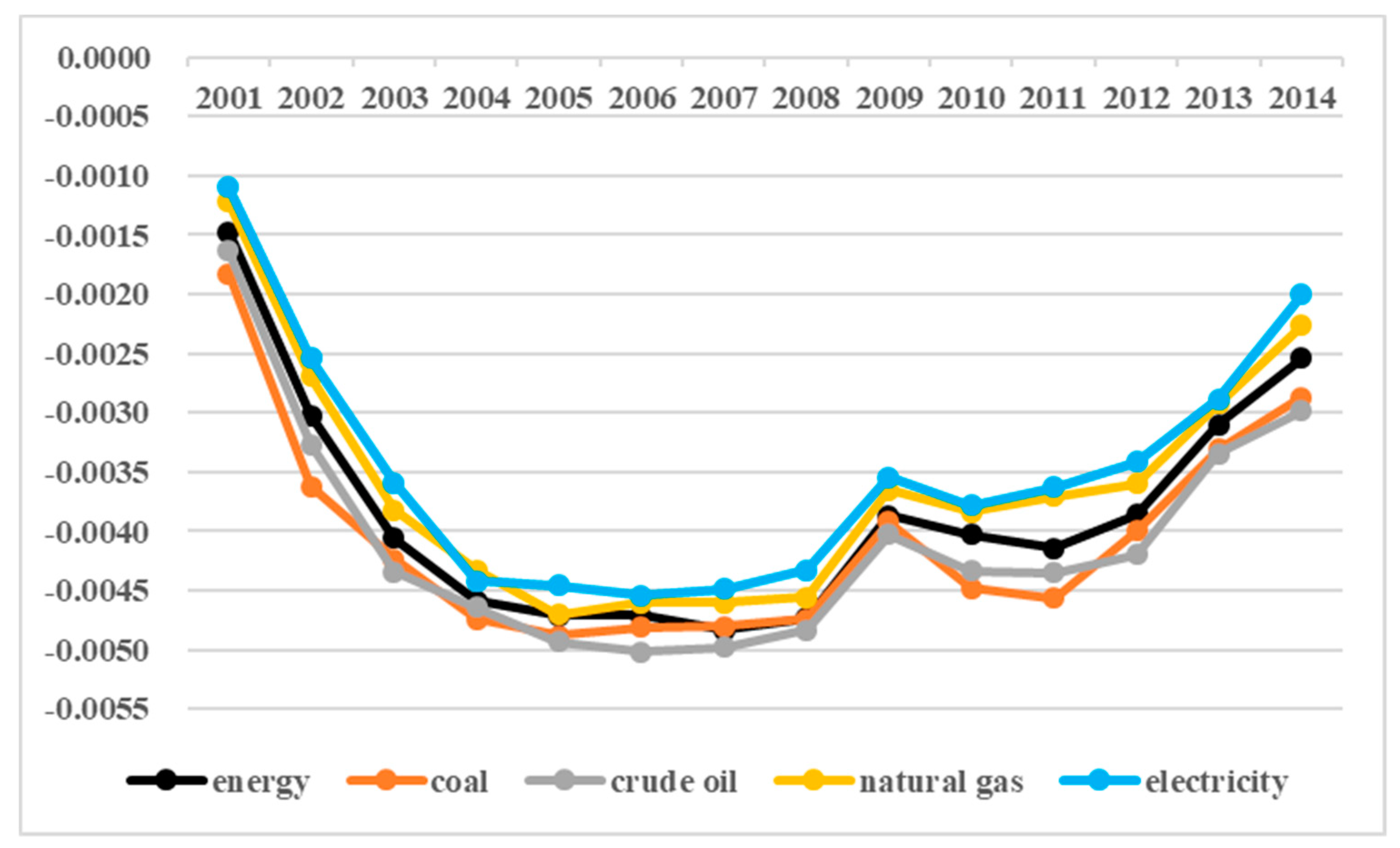
Technical change’s capital–energy bias (biasKE) is the primary independent variable in the panel model. Its measurement is important to the estimation. The proxy for energy (E) employed above is the total energy consumption.
To check its robustness, four other proxies are used for the energy: coal consumption, crude oil consumption, natural gas consumption, and electricity consumption, and the technical change’s capital–energy bias is re-estimated. Figure 5 reports the estimation results using different proxies for energy. Technical change’s capital–energy bias was smaller than 0 during the observation period, and has increased substantially. That is, technical change in China is indeed energy-biased, and the gap between capital and energy has gradually diminished since 2007. Different estimations are quite close to each other in both magnitude and tendency. Using different proxies for energy would not affect the estimation on technical change’s capital–energy bias. The estimation result using the total energy consumption is robust.
6. Conclusions and Policy Implications
According to this paper’s findings, China’s total factor carbon emissions efficiency still has a large room for improvement. Carbon emissions efficiency varies a lot across regions. Eastern area boasts the highest efficiency, while other areas do not perform well during the observation period. For an active government, more attempts need to be made to help the nation to get out of the current carbon emissions dilemma in the context of global climate change.
Technical change’s increasing capital–energy bias substantially improves China’s carbon emissions efficiency. After eliminating the endogeneity, the estimates are still robust. The mechanism behind is the changing factor substitution elasticity in the industry upgrade process. The structural transformation of manufacturing sector, popularization of higher education, R&D and foreign direct investment all positively affect carbon emissions efficiency. These are of significant value to policy makers who are seeking the solutions for improving carbon emissions efficiency.
Based on the findings, this paper puts forward the following policy recommendations. On the one hand, the economic growth goal should be adjusted actively to promote the economy to transit from an investment-driven pattern (extensive development) to an innovation-driven pattern (intensive development). Greater emphasis ought to be laid on achieving a balance between the economy and the environment, which is vital to realize sustainable development and green growth, characterized by high efficiency and low emissions. On the other hand, more policies could be implemented to enhance the upgrade of the industrial structure. The knowledge- and technology-intensive industry ought to be encouraged to increase capital’s marginal production growth rate, thus promoting the economy to transition to an energy-saving one.
Acknowledgments
The author is grateful for valuable comments from Zhi Li (Xiamen University), Rudai Yang (Peking University), and Xi Ji (Peking University).
Conflicts of Interest
The author declares no conflict of interest.
References
- Lin, B.; Li, J. The rebound effect for heavy industry: Empirical evidence from China. Energy Policy 2014, 74, 589–599. [Google Scholar] [CrossRef]
- Tol, R.S. Estimates of the damage costs of climate change. Part 1: Benchmark estimates. Environ. Resour. Econ. 2002, 21, 47–73. [Google Scholar] [CrossRef]
- Wang, B.; Qi, S. Biased technology progress, factor substitution and China's industrial energy intensity. Econ. Res. J. 2014, 2, 115–127. (In Chinese) [Google Scholar]
- Acemoglu, D. Directed Technical Change. Rev. Econ. Stud. 2002, 69, 781–809. [Google Scholar] [CrossRef] [Green Version]
- Popp, D. Induced Innovation and Energy Prices. Am. Econ. Rev. 2001, 92, 160–180. [Google Scholar] [CrossRef]
- Hassler, J.; Krusell, P.; Olovsson, C. Energy-Saving Technical Change; Social Science Electronic Publishing: Rochester, NY, USA, 2012. [Google Scholar]
- Wing, I.S. Representing induced technological change in models for climate policy analysis. Energy Econ. 2006, 28, 539–562. [Google Scholar] [CrossRef]
- Donadelli, M.; Grüning, P.; Jüppner, M.; Kizys, R. Global temperature, R&D, Expenditure and Growth. SAFE Working Paper n. 188. 2017. Available online: https://www.econstor.eu/bitstream/10419/171922/1/1006417478.pdf (accessed on 26 January 2019).
- Park, J. Will We Adapt? Temperature Shocks, Labor Productivity, and Adaptation to Climate Change in the United States (1986–2012); Harvard Project on Climate Agreements Discussion Paper Series 81; Harvard University: Cambridge, MA, USA, 2016. [Google Scholar]
- Donadelli, M.; Jüppner, M.; Riedel, M.; Schlag, C. Temperature shocks and welfare costs. J. Econ. Dyn. Control 2017, 82, 331–355. [Google Scholar] [CrossRef] [Green Version]
- Deschênes, O.; Greenstone, M. Climate change, mortality, and adaptation: Evidence from annual fluctuations in weather in the US. Am. Econ. J. Appl. Econ. 2011, 3, 152–185. [Google Scholar] [CrossRef]
- Burke, M.; Emerick, K. Adaptation to climate change: Evidence from US agriculture. Am. Econ. J. Econ. Policy 2016, 8, 106–140. [Google Scholar] [CrossRef]
- Ang, B.W. Is the energy intensity a less useful indicator than the carbon factor in the study of climate change? Energy Policy 1999, 27, 943–946. [Google Scholar] [CrossRef]
- Ramanathan, R. Combining indicators of energy consumption and CO2 emissions: A cross-country comparison. Int. J. Glob. Energy Issues 2002, 17, 214–227. [Google Scholar] [CrossRef]
- Zaim, O.; Taskin, F. Environmental efficiency in carbon dioxide emissions in the OECD: A non-parametric approach. J. Environ. Manag. 2000, 58, 95–107. [Google Scholar] [CrossRef] [Green Version]
- Chung, Y.H.; Färe, R.; Grosskopf, S. Productivity and Undesirable Outputs: A Directional Distance Function Approach. J. Environ. Manag. 1997, 51, 229–240. [Google Scholar] [CrossRef]
- Tone, K. Dealing with Undesirable Outputs in DEA: A Slacks-based Measure (SBM) Approach. 2003. Available online: https://ci.nii.ac.jp/naid/120005571101/ (accessed on 26 January 2019).
- Zhou, P.; Ang, B.W.; Poh, K.L. Slacks-based efficiency measures for modeling environmental performance. Ecol. Econ. 2006, 60, 111–118. [Google Scholar] [CrossRef]
- Zhang, B.; Bi, J.; Fan, Z.; Yuan, Z.; Ge, J. Eco-efficiency analysis of industrial system in China: A data envelopment analysis approach. Ecol. Econ. 2008, 68, 306–316. [Google Scholar] [CrossRef]
- Wang, K.; Wei, Y.M.; Zhang, X. A comparative analysis of China’s regional energy and emission performance: Which is the better way to deal with undesirable outputs? Energy Policy 2012, 46, 574–584. [Google Scholar] [CrossRef]
- Zhou, P.; Ang, B.W.; Wang, H. Energy and CO2 emission performance in electricity generation: A non-radial directional distance function approach. Eur. J. Oper. Res. 2012, 221, 625–635. [Google Scholar] [CrossRef]
- Lin, B.; Du, K. Energy and CO2 emissions performance in China’s regional economies: Do market-oriented reforms matter? Energy Policy 2015, 78, 113–124. [Google Scholar] [CrossRef]
- Yin, K.; Wang, R.; An, Q.; Yao, L.; Liang, J. Using eco-efficiency as an indicator for sustainable urban development: A case study of Chinese provincial capital cities. Ecol. Indic. 2014, 36, 665–671. [Google Scholar] [CrossRef] [Green Version]
- Li, K.; Lin, B. Economic growth model, structural transformation, and green productivity in China. Appl. Energy 2017, 187, 489–500. [Google Scholar] [CrossRef]
- Kemfert, C.; Welsch, H. Energy-Capital-Labor Substitution and the Economic Effects of CO2 Abatement: Evidence for Germany. J. Policy Model. 2000, 22, 641–660. [Google Scholar] [CrossRef]
- Popp, D. The effect of new technology on energy consumption. Resour. Energy Econ. 2001, 23, 215–239. [Google Scholar] [CrossRef] [Green Version]
- Welsch, H.; Ochsen, C. The determinants of aggregate energy use in West Germany: Factor substitution, technological change, and trade. Energy Econ. 2005, 27, 93–111. [Google Scholar] [CrossRef]
- Fisher-Vanden, K.; Jefferson, G.H. Technology diversity and development: Evidence from China's industrial enterprises. J. Comp. Econ. 2008, 36, 658–672. [Google Scholar] [CrossRef] [Green Version]
- Chen, X.; Xu, S.; Lian, Y. Factor substitution elasticity and biased technology’s effects on industrial energy intensity. J. Quant. Tech. Econ. 2015, 3, 58–76. (In Chinese) [Google Scholar]
- Färe, R.; Grosskopf, S.; Pasurka, C.A., Jr. Environmental production functions and environmental directional distance functions. SSRN Electron. J. 2007, 32, 1055–1066. [Google Scholar] [CrossRef]
- Lozano, S.; Gutiérrez, E. Non-parametric frontier approach to modelling the relationships among population, GDP, energy consumption and CO2 emissions. Ecol. Econ. 2008, 66, 687–699. [Google Scholar] [CrossRef]
- Wang, Q.; Zhou, P.; Zhou, D. Efficiency measurement with carbon dioxide emissions: The case of China. Appl. Energy 2012, 90, 161–166. [Google Scholar] [CrossRef]
- Werf, E.V.D. Production functions for climate policy modeling: An empirical analysis. Energy Econ. 2008, 30, 2964–2979. [Google Scholar] [CrossRef] [Green Version]
- Diamond, P.A. Disembodied technical change in a two-sector model. Rev. Econ. Stud. 1965, 32, 161–168. [Google Scholar] [CrossRef]
- Hao, F. Formula correction and estimation methods comparison on elasticity of substitution within translog function. J. Quant. Tech. Econ. 2015, 4, 88–105. [Google Scholar]
- Zhou, X.; Zhang, J.; Li, J. Industrial structural transformation and carbon dioxide emissions in China. Energy Policy 2013, 57, 43–51. [Google Scholar] [CrossRef]
- Lin, B.; Ouyang, X. A revisit of fossil-fuel subsidies in china: Challenges and opportunities for energy price reform. Energy Convers. Manag. 2014, 82, 124–134. [Google Scholar] [CrossRef]
- Gireesh, N.; Leif, G.; Krushna, M. Factors influencing energy efficiency investments in existing Swedish residential buildings. Energy Policy 2010, 38, 2956–2963. [Google Scholar]
- Poortinga, W.; Steg, L.; Vlek, C.; Wiersma, G. Household preferences for energy-saving measures: A conjoint analysis. J. Econ. Psychol. 2003, 24, 49–64. [Google Scholar] [CrossRef]
- Lee, K.H.; Min, B. Green R&D for eco-innovation and its impact on carbon emissions and firm performance. J. Clean. Prod. 2015, 108, 534–542. [Google Scholar] [Green Version]
- Lee, J.W. The contribution of foreign direct investment to clean energy use, carbon emissions and economic growth. Energy Policy 2013, 55, 483–489. [Google Scholar] [CrossRef]
- Diakoulaki, D.; Mandaraka, M. Decomposition analysis for assessing the progress in decoupling industrial growth from CO2 emissions in the EU manufacturing sector. Energy Econ. 2007, 29, 636–664. [Google Scholar] [CrossRef]
- Song, M.; Wang, S.; Cen, L. Comprehensive efficiency evaluation of coal enterprises from production and pollution treatment process. J. Clean. Prod. 2015, 104, 374–379. [Google Scholar] [CrossRef]
- Liu, H.; Lin, B. Ecological indicators for green building construction. Ecol. Indic. 2016, 67, 68–77. [Google Scholar] [CrossRef]
- Shan, H. Re-estimating the capital stock of China: 1952–2006. J. Quant. Tech. Econ. 2008, 10, 17–31. (In Chinese) [Google Scholar]
- Wu, Y. Productivity, Efficiency and Economic Growth in China; Palgrave Macmillan: Basingstoke, UK, 2008. [Google Scholar]
- Intergovernmental Panel on Climate Change (IPCC). IPCC Guidelines for National Greenhouse Gas Inventories; Intergovernmental Panel on Climate Change: London, UK, 2006. [Google Scholar]
- Bai, J.; Jiang, K.; Li, J. On the efficiency and total factor productivity growth of China’s R&D innovation. J. Quant. Tech. Econ. 2009, 3, 139–151. (In Chinese) [Google Scholar]
- Wu, Y. Indigenous R&D, technology imports and productivity: Evidence from industries across regions of China. Econ. Res. J. 2008, 8, 51–64. (In Chinese) [Google Scholar]
- Hall, B.H.; Mairesse, J. Exploring the relationship between R&D and productivity in French manufacturing firms. J. Econom. 1995, 65, 263–293. [Google Scholar]
- Moore, J.H. A measure of structural change in output. Rev. Income Wealth 1978, 24, 105–118. [Google Scholar] [CrossRef]
Figure 1.
China’s regional total factor carbon emissions efficiency during 2001–2014.

Figure 2.
China’s biased technical change during 2001–2014. Note: Technical change’s capital–labor bias (biasKL) and energy–labor bias (biasEL) are measured by the left-side coordinate system, while capital–energy bias (biasKE) is measured by the right-side coordinate system.
Figure 2.
China’s biased technical change during 2001–2014. Note: Technical change’s capital–labor bias (biasKL) and energy–labor bias (biasEL) are measured by the left-side coordinate system, while capital–energy bias (biasKE) is measured by the right-side coordinate system.
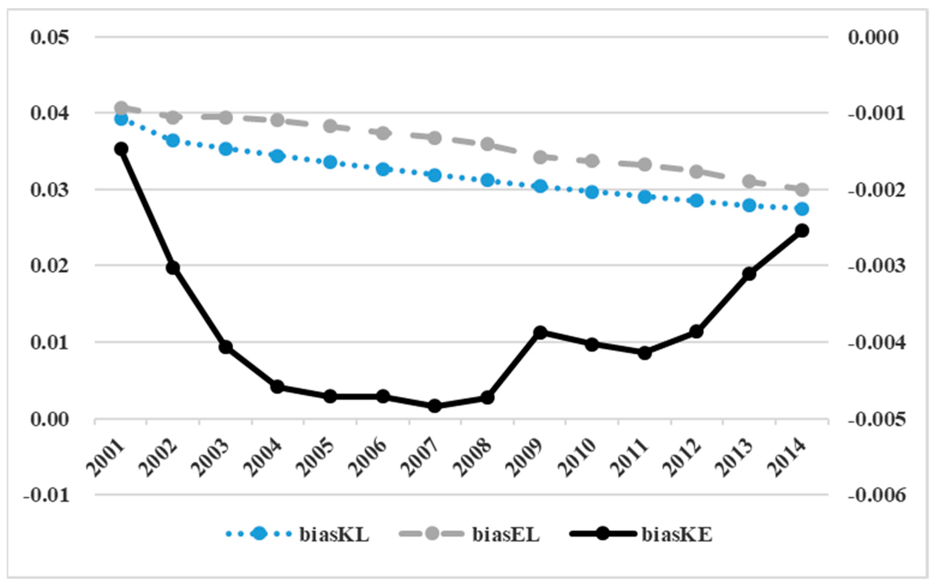
Figure 3.
China’s factor substitution elasticity in 2001–2014. Note: Energy–labor substitution elasticity (E-L) is measured by the left-side coordinate system, while capital–labor substitution elasticity (K–L), and capital–energy substitution elasticity (K–E) are measured by the right-side coordinate system.
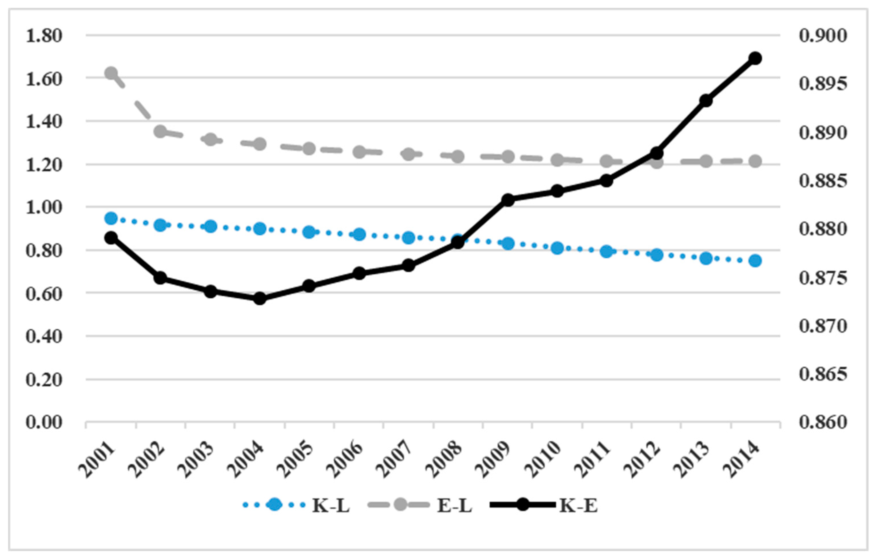
Figure 4.
Mechanism of biased technical change’s impact on carbon emissions efficiency.
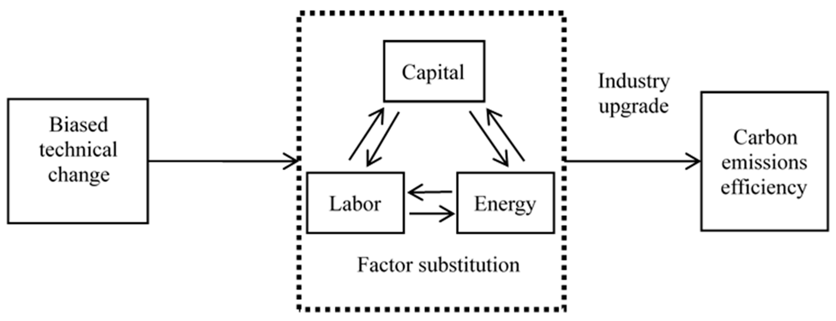
Figure 5.
Estimation on technical change’s capital–energy bias using different proxies for energy.

Table 1.
Carbon dioxide emissions coefficients.
| Sources | Coal | Coke | Gasoline | Kerosene | Crude oil | Fuel oil | Gas | Cement |
| coefficients | 1.647 | 2.848 | 3.045 | 3.174 | 3.150 | 3.064 | 21.670 | 0.527 |
Source: [47].
Table 2.
Descriptive statistics.
| Variables | Units | Mean | Std. Dev. | Min | Max |
|---|---|---|---|---|---|
| Labor (L) | Million workers | 24.42 | 16.38 | 2.78 | 66.15 |
| Capital stock (K) | RMB billion (Constant 2001 price) | 790.27 | 754.07 | 19.58 | 4431.17 |
| Energy consumption (E) | Million tons of coal equivalent | 105.94 | 74.66 | 5.20 | 388.99 |
| Real gross domestic product (GDP) | RMB billion (Constant 2001 price) | 933.96 | 895.13 | 30.01 | 5089.54 |
| CO2 emissions (CE) | Million tons | 299.82 | 220.45 | 18.88 | 1099.69 |
| Industrial structural transformation (ois) | \ | 0.1198 | 0.0876 | 0 | 0.3566 |
| Energy price (price) | base = 100 | 174.41 | 52.90 | 97.1 | 301.64 |
| Popularization of higher education (edu) | % | 0.33 | 0.19 | 0.04 | 0.87 |
| R&D stock (rd) | RMB billion (Constant 2001 price) | 53.78 | 76.38 | 0.44 | 434.82 |
| FDI stock (fdi) | RMB billion (Constant 2001 price) | 117.53 | 159.53 | 0.73 | 780.25 |
| Value added of industry (ivalue) | RMB billion (Constant 2001 price) | 234.7 | 296.6 | 6.53 | 1671.9 |
Table 3.
Estimates for effect of biased technical change on carbon emissions efficiency.
| TFCE | (1) FGLS | (2) FGLS | (3) FGLS | (4) FGLS | (5) Diff-GMM |
|---|---|---|---|---|---|
| biasKE | 6.3817 *** (1.6728) | 4.5690 *** (0.4982) | 3.9246 *** (0.9901) | 4.1922 *** (0.9380) | 2.8219 *** (0.7258) |
| ois | 0.4788 *** (0.1519) | 0.3521 *** (0.1210) | 0.3274 *** (0.1141) | 0.3057 *** (0.0626) | |
| price | −0.0040 *** (0.0005) | −0.0007 *** (0.0002) | −0.0002 (0.0003) | −0.0003 (0.0008) | |
| edu | 0.2629 *** (0.0714) | 0.2975 *** (0.0656) | 0.2391 ** (0.0525) | 0.2869 *** (0.0502) | |
| rd | 0.0012 *** (0.0004) | 0.0009 *** (0.0003) | 0.0008 *** (0.0002) | 0.0009 *** (0.0003) | |
| fdi | 0.0006 *** (0.0002) | 0.0004 ** (0.0002) | 0.0004 ** (0.0002) | 0.0003 ** (0.0001) | |
| ivalue | −0.0005 ** (0.0002) | −0.0004 ** (0.0002) | −0.0004 ** (0.0002) | −0.0003 * (0.0002) | |
| province fixed effect | No | No | Yes | Yes | |
| year fixed effect | No | No | No | Yes | |
| Lag.TFCE | 0.5833 ** (0.2663) | ||||
| Constant | 0.4625 *** (0.0280) | 0.2553 *** (0.0511) | 0.3020 *** (0.0592) | 0.3029 *** (0.0616) | |
| R2 | 0.0494 | 0.5312 | 0.8911 | 0.8961 | |
| AR (1) test | 0.1626 [0.0021] | ||||
| AR (2) test | 0.0480 [0.3371] | ||||
| Sargan test | 25.1189 [0.2420] | ||||
| Sample | 420 | 420 | 420 | 420 | 360 |
Note: Robust standard errors clustered at the province level are obtained by the bootstrapped method based on 50 replications, and they are presented in parentheses. p-values of test statistics are in square brackets. * Statistical significance at the 10% level. ** Statistical significance at the 5% level. *** Statistical significance at the 1% level.
Table 4.
Estimates for interaction impact of biased technical change and industrial structural transformation on carbon emissions efficiency.
Table 4.
Estimates for interaction impact of biased technical change and industrial structural transformation on carbon emissions efficiency.
| TFCE | (1) FGLS | (2) FGLS | (3) FGLS | (4) FGLS | (5) Diff-GMM |
|---|---|---|---|---|---|
| biasKE | 5.0261 *** (1.8573) | 4.1249 *** (0.9555) | 3.6657 *** (0.9928) | 3.8263 *** (0.9528) | 2.7293 *** (0.7046) |
| ois | 0.3163 *** (0.1162) | 0.4032 ** (0.2006) | 0.3556 ** (0.1489) | 0.3760 ** (0.1634) | 0.3090 ** (0.1232) |
| biasKE × ois | 1.8792 *** (0.2411) | 1.2243 *** (0.3801) | 1.5282 *** (0.5305) | 1.5136 *** (0.5121) | 1.4729 *** (0.4646) |
| other control variables | No | Yes | Yes | Yes | Yes |
| province fixed effect | No | No | Yes | Yes | |
| year fixed effect | No | No | No | Yes | |
| Lag.TFCE | 0.4906 ** (0.2106) | ||||
| Sample | 420 | 420 | 420 | 420 | 360 |
Note: Robust standard errors clustered at the province level are obtained by the bootstrapped method based on 50 replications, and they are presented in parentheses. p-values of test statistics are in square brackets. * Statistical significance at the 10% level. ** Statistical significance at the 5% level. *** Statistical significance at the 1% level.
© 2019 by the author. Licensee MDPI, Basel, Switzerland. This article is an open access article distributed under the terms and conditions of the Creative Commons Attribution (CC BY) license (http://creativecommons.org/licenses/by/4.0/).
Share and Cite
MDPI and ACS Style
Zhong, J. Biased Technical Change, Factor Substitution, and Carbon Emissions Efficiency in China. Sustainability 2019, 11, 955. https://doi.org/10.3390/su11040955
AMA Style
Zhong J. Biased Technical Change, Factor Substitution, and Carbon Emissions Efficiency in China. Sustainability. 2019; 11(4):955. https://doi.org/10.3390/su11040955
Chicago/Turabian StyleZhong, Jingdong. 2019. "Biased Technical Change, Factor Substitution, and Carbon Emissions Efficiency in China" Sustainability 11, no. 4: 955. https://doi.org/10.3390/su11040955
Note that from the first issue of 2016, this journal uses article numbers instead of page numbers. See further details here.