Experimental Study on Hydromechanical Behavior of an Artificial Rock Joint with Controlled Roughness

Abstract

Rock mass contains various discontinuities, such as faults, joints, and bedding planes. Among them, a joint is one of the most frequently encountered discontinuities in rock engineering applications. Generally, a joint exerts great influence on the mechanical and hydraulic behavior of rock mass, since it acts as a weak plane and as a fluid path in the rock mass. Therefore, an accurate understanding on joint characteristics is important in many projects. In-situ tests on joints are sometimes consumptive in terms of time and expenses so that the features are investigated by laboratory tests, providing fundamental properties for rock mass analyses. Although the behavior of a joint is affected by both mechanical and geometric conditions, the latter are often limited, since quantitative control on the conditions is quite complicated. In this study, artificial rock joints with various geometric conditions, i.e., joint roughness, were prepared in a quantitative manner and the hydromechanical characteristics were investigated by several laboratory experiments. Based on the results, a prediction model for hydraulic aperture was proposed in the form of ${(e_h/e_m)}^3=\exp (-0.0462c)\times {(0.8864)}^{JRC}$, which was a function of the mechanical aperture, joint roughness, and contact area. Relatively good agreement between the experimental results and predicted value indicated that the model is capable of estimating the hydraulic aperture properly.

1. Introduction

Rock mass contains various types of discontinuities in terms of size and shape, such as faults, joints, and bedding planes. Among them, a joint is a planar discontinuity that has little tensile strength showing smaller size, but more frequency than a fault. Generally, a joint exerts great influence on the mechanical behavior of rock mass, since it acts as a weak plane. At the same time, a joint has several orders higher hydraulic conductivity than rock matrix so that the majority of fluid flow in rock mass takes place through the joint [1,2,3]. Therefore, it is necessary to take hydromechanical characteristics of joint into account in many rock engineering applications.

For instance, in many rock engineering applications, including radioactive waste disposal [4,5], geothermal energy extraction [5,6], geological CO₂ sequestration, and deep underground tunneling, it is essential to accurately understand the hydromechanical behavior of rock joints so as to secure the stability and the efficiency of the projects. In-situ experiments can measure hydromechanical characteristics of rock mass, which consider the effects of multiple joints or joint sets. However, they are sometimes consumptive in terms of time and expenses so that the features are investigated by laboratory experiments on a joint, providing fundamental properties for rock mass analyses.

In many cases, joints are originated and gone through several geological processes under various geological conditions. A fracture void, which is a space between corresponding joint surfaces, is characterized by several joint properties, such as roughness, aperture, stiffness, contact area, etc. [7,8]. They exert complex influence on the hydromechanical characteristics of the joint, interacting with each other. Mechanical aperture is the distance between two corresponding joint surfaces in the direction perpendicular to the reference plane of the joint [7], while hydraulic aperture is calculated value based on the results of flow test. The aperture acts as a flow path in a joint, thus, several researches investigated relationships between the aperture and other joint properties [9,10,11]. Roughness has drawn attentions for the relationship, since it is a widely used engineering parameter and relatively easy to be measured. The roughness is usually defined by its height distribution or shape of which the quantification can be made in several different roughness parameters.

An artificial joint specimen is often used to conduct the laboratory experiments. The joint specimen is bisected mechanically by using a splitter or V block, which is similar to Brazilian jaws [3,12,13]. Although it is a simple method to create the joint specimens, it requires excessive efforts if a specific roughness is required. Therefore, some experimental works are derived from limited test conditions in terms of the joint roughness, which are mainly due to the difficulties in specimen preparation [12,13,14,15,16]. Reproducibility of this approach is hardly guaranteed. Therefore, casting method, which usually uses cement mortar or epoxy, is adopted as an alternative to make multiple joint specimens having similar value of roughness [17,18]. In many cases, however, the casting method also requires some joints at the early stage, since it needs original joint surfaces to make molding frames. Though it can remedy the reproducibility problem to some extent, quantitative control on the geometric property of joint is still incomplete.

In this study, a series of laboratory experiments were carried out to investigate the hydromechanical characteristics of an artificial rock joint under various experimental conditions. In order to control the joint roughness in a quantitative manner, a fractal theory, specifically the random midpoint displacement method, was adopted to mathematically define the joint surfaces. By manipulating input parameters of the method, point-cloud type data of the joint surfaces were produced with various levels of roughness. Then, the data, which contained coordinates of surface points, were imported to a 3D printer. Thanks for the recent development in 3D printing technology, laborious works in specimen preparation can be avoided to some degree. Throughout this paper, a whole experiment scheme could be classified into three parts. First, geometric properties of joint, i.e., roughness, aperture, and fracture void, were investigated. Surface information of joint was measured by a 3D laser scanner and utilized in the following experimental steps. Second, mechanical characteristics of the joint were measured by normal compression tests. Under the applied normal load, deformation behavior and corresponding variation of fracture void could be investigated. Last, flow tests were conducted under normal compression. With an assumption of cubic law, the variation of hydraulic (or equivalent) aperture under various geometric and mechanical conditions was figured out. Sufficient experimental condition was applied in terms of stress and roughness so as to obtain wide applicability and representativeness from the experiments.

Hydraulic conductivity of a joint is an important property in rock mass analyses and can be expressed in terms of hydraulic aperture. Therefore, several prediction models were proposed for estimating the hydraulic aperture [19,20,21]. They have their own strength and shortcomings, being bound in some cases by their own definitions. In this study, a prediction model was proposed based on the experimental results. The model was derived by multivariable, nonlinear regression analyses and was established as a function of mechanical aperture, roughness, and contact area. In order to confirm the validity and applicability of the model, comparison with the referenced models was made. It was found that the model showed acceptable predictability in engineering viewpoint.

2. Experimental Setup

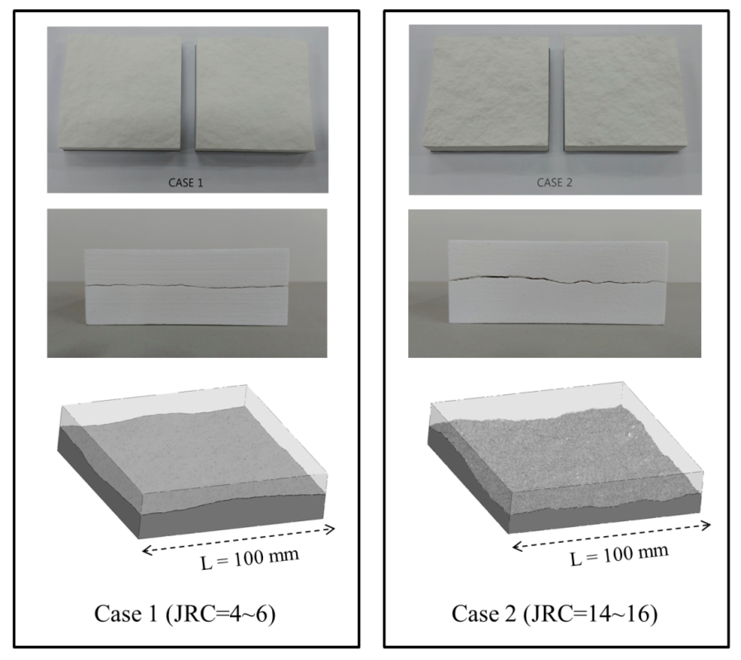
Several methodologies were suggested to mathematically define an artificial joint surface. Fourier transformation [22], stochastic function, such as autocorrelation function [23], and fractal Brownian function [24] can be adopted in this procedure. In 1993, Xie [24] stated that rock joints could be successfully simulated by the fractal theory in terms of roughness, aperture, pore structure, permeability, etc. Natural rock joints usually show self-affinity, which is the feature that considers different amount of scaling in transformation. The fractal Brownian functions could take the feature into account, thus, it can be applied in estimating and/or generating models of artificial joint surfaces. In this study, random midpoint displacement method was adopted to generate synthetic surfaces. It has several benefits in application. First, it is quite straightforward, and its outcomes can be directly imported to a 3D printer. Also, the manipulation of input parameters can derive satisfactory results in controlling joint roughness [25]. Figure 1 shows an example of the printed joint specimens following the method. The uppermost pictures in Figure 1 show two corresponding joint surfaces (upper and lower), which were printed by a 3D printer, and the middle pictures show joint-embedding specimen, piling up those two surfaces to be mated. The last pictures show 3D numerical models, which had the same geometry with the printed specimens.

In 2019, Choi et al. reported that the method could give satisfactory results in controlling the joint roughness, which was expressed in $JRC$ (Joint Roughness Coefficient). In 1977, Barton and Choubey [26] proposed the roughness parameter by back-calculating numerous direct shear test results. Although $JRC$ is not a quantitative parameter, it is widely used in engineering projects mainly due to its simplicity and practicability. Therefore, it was selected as a roughness estimator in this study. Figure 1 is an example to show how well the method controls the joint roughness. Actual laboratory experiments were conducted using cylindrical specimens, not rectangular parallelepiped as shown in Figure 1. The procedure for specimen preparation is described below.

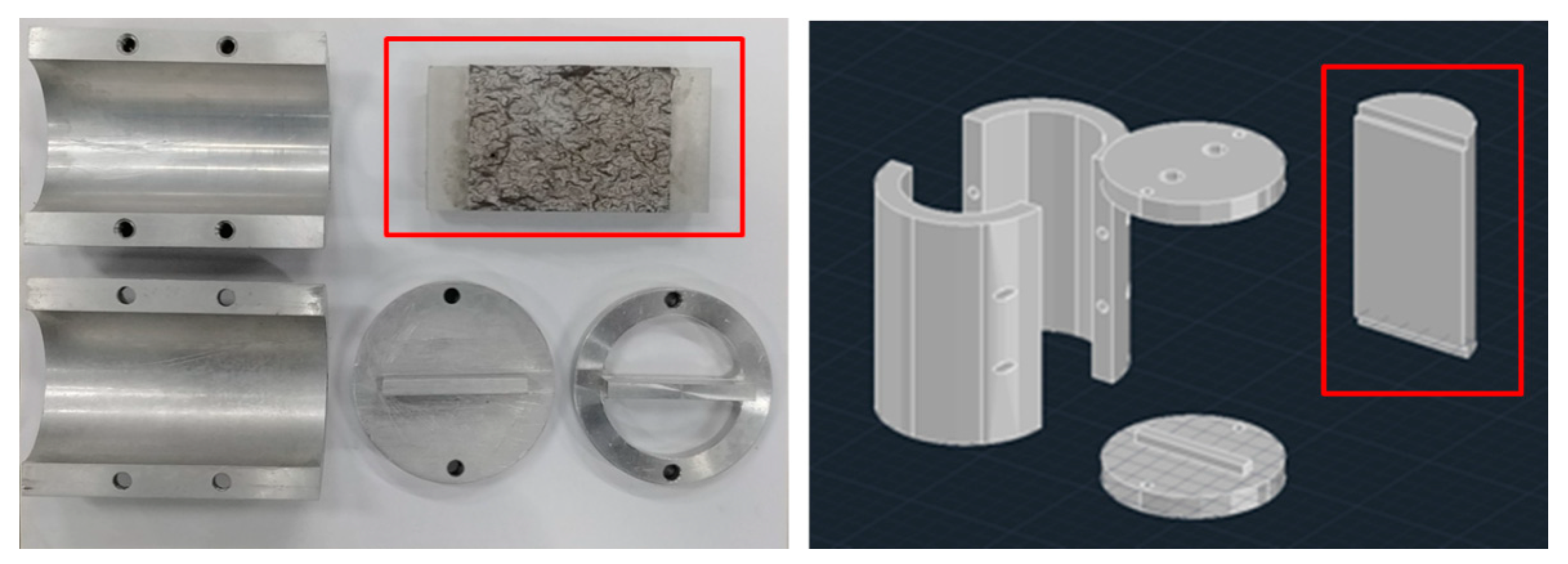
The 3D printer used in this study was an ‘additive manufacturing’ type and, more precisely speaking, a binding jetting printer. It spreads a liquid state additive onto powder layer to embody predesigned objects. It is capable of making complex shape and colored objects, however, mechanical and physical properties of the printed outcome are highly dependent on printing ingredients. Unfortunately, the printer uses calcium sulfate hemihydrate powder as a main printing ingredient, which is inadequate to make a rock-like specimen in terms of strength and stiffness. Therefore, the printer produced prototype joint surfaces first. Then several aluminum casting molds, which had similar degree of roughness, were manufactured based on the prototype surfaces. Figure 2 shows the whole molding assembly including the aluminum casting mold. Joint specimens were made of cement mortar using the molding assembly, which had a cement/water ratio of 100:20 by weight with the addition of little retarder. After the whole assembly put together, cement mortar was poured into the assembly to make a half of a joint. After 5–6 h of curing, the assembly was carefully dismantled. Then, the molds were reassembled incorporating the half of the joint instead of the aluminum mold. Cement mortar was poured again to make another half of the joint. Then, the assembly was taken apart. After carefully detaching the two halves of the joint, the specimens were cured more than three days to guarantee material strength under room temperature and humidity. The specimens had 54 mm of dimeter and a ratio of height to diameter was approximately 2. However, the specimen should contain some margin at the upper and lower parts so that the actual area of joint surface was 75 mm × 54 mm. In order to investigate the effects of roughness, four joint specimens having different roughness were prepared and tested throughout this study.

In order to obtain and confirm geometric information of the joint surface, i.e., roughness, aperture, and shape of fracture void, a 3D laser scanner was used. As a non-contact measuring method, it can provide x, y, and z coordinates of surface points without any damage. Thus, many researches adopt this technique [3,12]. As mentioned above, the original surfaces were generated by the the random midpoint displacement method, however, some inevitable degradation of micro asperity occurred when manufacturing the aluminum casting mold. Therefore, there existed discrepancies between the generated surface and the cement mortar joint surface. Hence, the joint specimens were scanned again to determine the geometric properties. Joint surface of 75 mm x 54 mm was scanned and digitized with scanning interval of 0.25 mm.

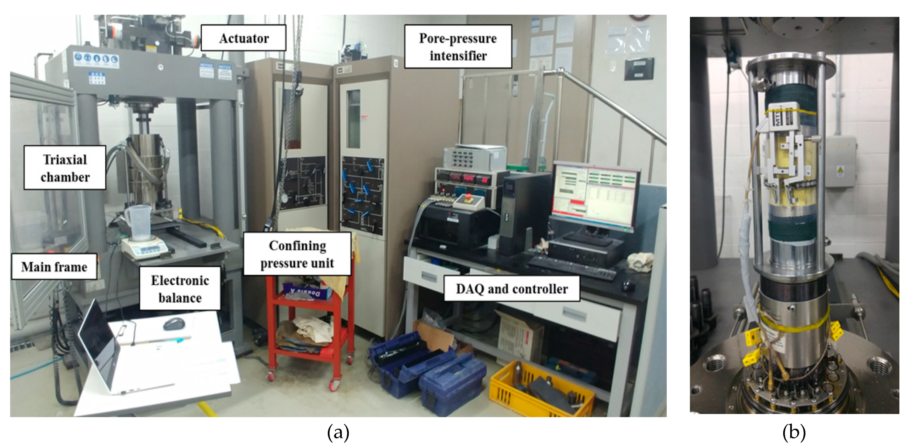
Figure 3 shows the experimental setup. MTS 816 system (universal rock testing system) was used in both mechanical and hydraulic experiments. It is composed of load frame (main frame), triaxial compression unit, pore pressure intensifier, and additional accessories (Figure 3a). An actuator, which locates at the top of main frame, typically applies and controls the axial displacement or stress during experiments. In this case, axial stress of 0.1 MPa was applied to fix the specimen assembly and was servo-controlled during the whole test. The triaxial compression unit consists of triaxial compression chamber and confining pressure unit. The triaxial compression chamber, in which the in-vessel test assembly is placed, is filled with refined oil and connected to the confining pressure unit. Since the axial (vertical) stress is constrained by the actuator, the confining pressure unit applies and controls diametrical stress, which acts as normal stress on the joint surface. The pore pressure intensifier applies and controls the hydraulic pressure and it is connected to the in-vessel assembly through a pair of endcaps. Fluid injected by the intensifier (distilled water, in this case) moves into the specimen through the lower endcap and is discharged through the upper endcap. The discharged fluid is weighed by an electronic balance. Figure 3b shows the in-vessel test assembly. A pair of endcaps is located at the top and bottom parts of the joint specimen being connected to the pore pressure intensifier. Guide rods and plate are installed to prevent tilting or bending of the assembly with sufficient rigidity.

In normal compression tests, typical setting of uniaxial compression test was applied [27]. However, cylindrical joint specimen made by the molding assembly in Figure 2 is not suitable for normal compression, since it requires a special loading frame that is similar with Brazilian jaws, but has the exact same curvature with the specimen and may be affected by specimen arrangement. Therefore, rectangular parallelepiped specimens with the same joint characteristics and dimensions were prepared for this test. Normal stress was applied up to 10 MPa at the constant displacement loading rate of 0.005 mm/s. The stress level corresponded to the vertical in-situ stress at the depth of approximately 400 m. In addition, two loading-unloading cycles were adopted to investigate the effect of stress hysteresis. After reaching normal stress of 10 MPa under the constant loading rate, the stress was removed then the second loading cycle began. Meanwhile, a flow test was conducted in a triaxial compression chamber. In the test, a cylindrical specimen with the attachment of two endcaps was placed inside of the chamber. Normal stress on the joint surface was applied and controlled by the confining pressure unit. Applied normal stress varied from 1 MPa to 10 MPa, with the interval of 1 MPa. The pore pressure intensifier-controlled water pressure at 0.3, 0.6, and 1.0 MPa. After the target normal and water pressure were applied, fluid injection was continued until it reached constant flowrate. Two loading cycles were applied in the flow tests as well.

3. Experimental Results

3.1. Geometric Properties of Joint Surface

Artificial joint specimens with four different levels of roughness were prepared. The specimens hereinafter are referred as J1, J2, J3, and J4, respectively. They were scanned by a high-resolution laser scanner and provided with the coordinates of surface points, allowing quantitative estimation on the roughness and mechanical aperture to be made. Various studies proposed quantitative roughness parameters and their relationships with $JRC$. For instance, in 1979, Tse and Cruden [28] suggested roughness parameter $Z_2$ (Equation (1)) and the relationship with $JRC$ (Equation (2)).

$$Z_2=\sqrt{\frac{1}{L}{\displaystyle {\int }_0^L{\left(\frac{dy}{dx}\right)}^{2}dx}}=\sqrt{\frac{1}{L}{\displaystyle \sum _{i=1}^{n-1}\frac{{(y_{i+1}-y_i)}^2}{x_{i+1}-x_i}}}$$

(1)

$$JRC=32.2+32.47\log Z_2$$

(2)

where $L$ is the length of a joint profile, $dx$ and $dy$ are the increments of x and y of the profile, $n$ is the number of segments, and $x_i$ and $y_i$ are the x and y coordinates of i th segment, respectively.

Several quantitative parameters, including $Z_2$, are two-dimensional in their nature. Obviously, representativeness of a single profile is insufficient for a whole joint surface, since the joint itself is a three-dimensional structure. A few three-dimensional parameters were suggested for better representativeness and taking roughness anisotropy into consideration [29,30]. However, their practicality could not have exceeded those of two-dimensional parameters.

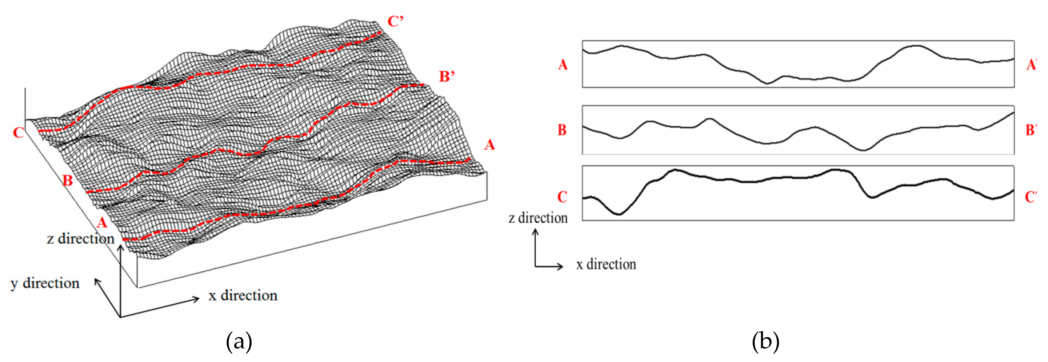
In this study, a compromise method was adopted in determining the joint roughness. Figure 4 shows a schematic diagram for the determination. Since all coordinates of surface points were already known, each and every profile along a certain direction could be obtained. In this study, the roughness along the long axis of a joint (x direction in Figure 4) was calculated. A joint profile would be defined by xz plane. Then, moving the xz plane along the y direction would define several profiles. Applying Equations (1) and (2) on the profiles in sequence would give a distribution of roughness so that the applicability of $JRC$ and three-dimensional feature could be enhanced. Average of the distribution was selected as a typical value.

The scanned coordinates could be utilized in determining the mechanical aperture as well. Several methodologies have been proposed to measure the mechanical aperture of a joint. Among them, superposition method was applied in this study. After arranging the coordinates of the upper and lower surfaces vertically, the upper surface was moved in parallel downward step-by-step until it met a certain criterion of aperture determination. When the criterion was met, the distances of all corresponding points were calculated to establish its distribution. The criterion was defined when 1% of the total surface points were in contact. It was referenced from the experimental results that the area contacted by the dead weight of the joint was approximately 1% of total surface [31]. Since only gravitational force exists, it is called initial mechanical aperture ($e_{m0}$). When superposing, the upper surface was translated downward by 0.001 mm at a step. Then, the distribution of aperture was calculated and all apertures in contact were set to null. Average of the distribution was selected as a typical value as well.

Five sets of specimens (a set consists of J1, J2, J3, and J4) were prepared and analyzed.

Table 1. Statistics of joint roughness and initial mechanical aperture.

Specimen	$\mathbf{Roughness}\left(\mathit{J}\mathit{R}\mathit{C}\right)$			Initial Mechanical Aperture (mm)
	Average	S.D.	CV (%)	Average	S.D.	CV (%)
J1	1.12	0.12	10.71	0.17	0.03	17.65
J2	7.32	0.59	8.06	0.39	0.09	23.08
J3	13.07	1.38	10.56	0.55	0.13	23.64
J4	16.47	1.46	8.86	0.82	0.17	20.73

shows weighted statistics of all sets in terms of $JRC$ and initial mechanical aperture. CV in Table 1 denotes coefficient of variation. Within applicable $JRC$ range, which is from 0 to 20, the roughness distributed relatively equally. And judging from the CV values in the roughness, the proposed method on joint specimen preparation could give consistent results regarding joint roughness. Measured initial mechanical aperture varied in the range of 0.17~0.82 mm. CV values in the aperture were larger than those of roughness. It was attributed to the effect of micro asperity damage during molding process. As $JRC$ increased, the initial mechanical aperture increased as well so that a positive relationship could be found between them.

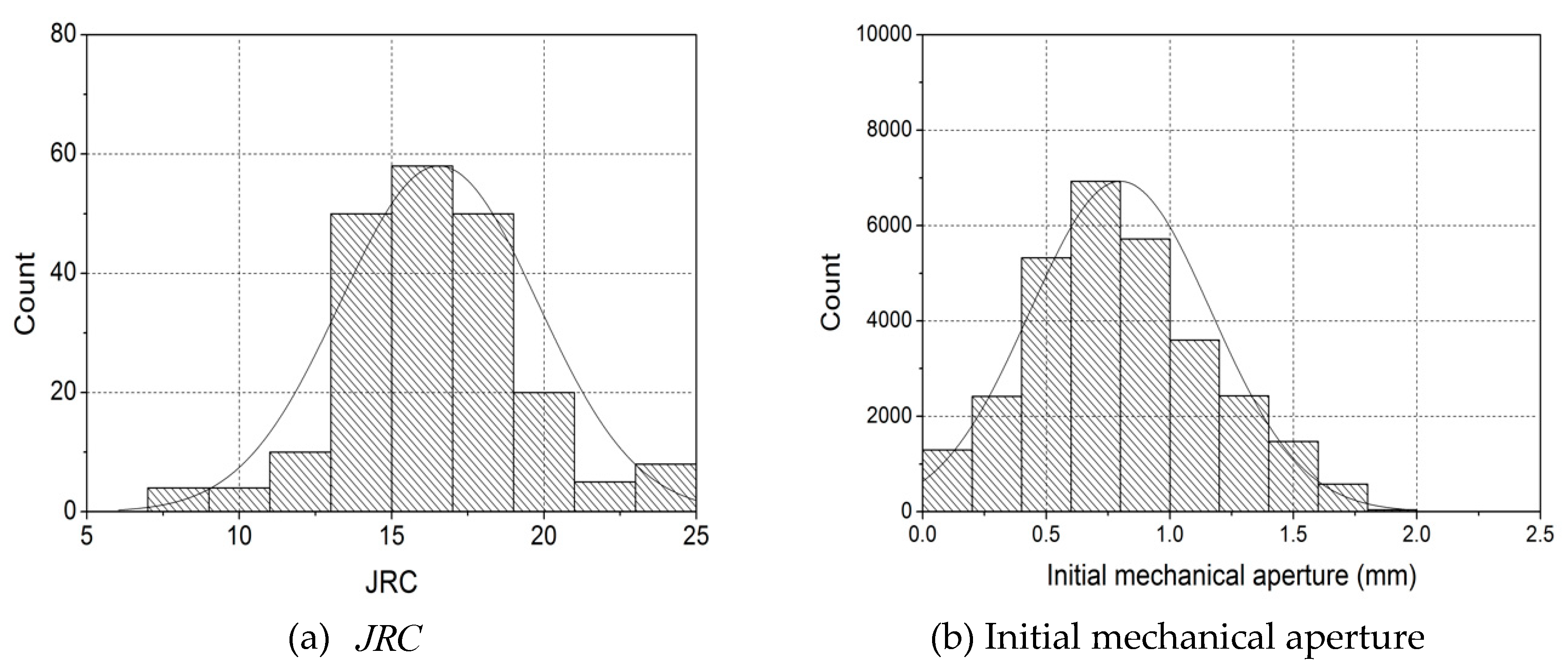
Figure 5 shows the distribution of $JRC$ and initial mechanical aperture as an example excerpted from J4. Curves in Figure 5 indicate fit normal distribution based on the results. Figure 5a shows that histogram of joint roughness followed normal distribution relatively well. However, some values were outside the applicable range of $JRC$ (larger than upper limit of 20). It was because the roughness was calculated by $Z_2$ (Equation (1)) first, which did not have numeric limitation on the contrary. The normal distribution on joint roughness could be explained by the surface generation algorithm, where Gaussian random number is involved. Random midpoint displacement method calculates elevation of asperity following the Gaussian distribution so that the roughness may show some normality in nature.

Distribution of initial mechanical aperture (Figure 5b) could be presented by normal distribution as well. Aperture of natural rock joint often follows a normal or log-normal distribution [4,32,33] and the same tendency could be found in this study. Since the specimens were made of cement mortar, there must be some discrepancies from real rock joints in terms of strength and stiffness. However, from a geometric viewpoint, it could be concluded that the proposed method for generating joint specimen was capable of simulating surface geometry of the rock joint.

3.2. Mechanical Characteristics

The specimens were made of cement mortar. In order to obtain fundamental properties of the testing material, uniaxial compression tests were conducted using 10 cylindrical intact specimens. As a result, uniaxial compressive strength and Young’s modulus were calculated as 48.15 MPa and 18.25 GPa on average, respectively. Therefore, the material was comparable with medium to weak strength rocks. Also, it was assumed that the material was more similar to sedimentary rocks than crystalline because of its texture of cemented grains.

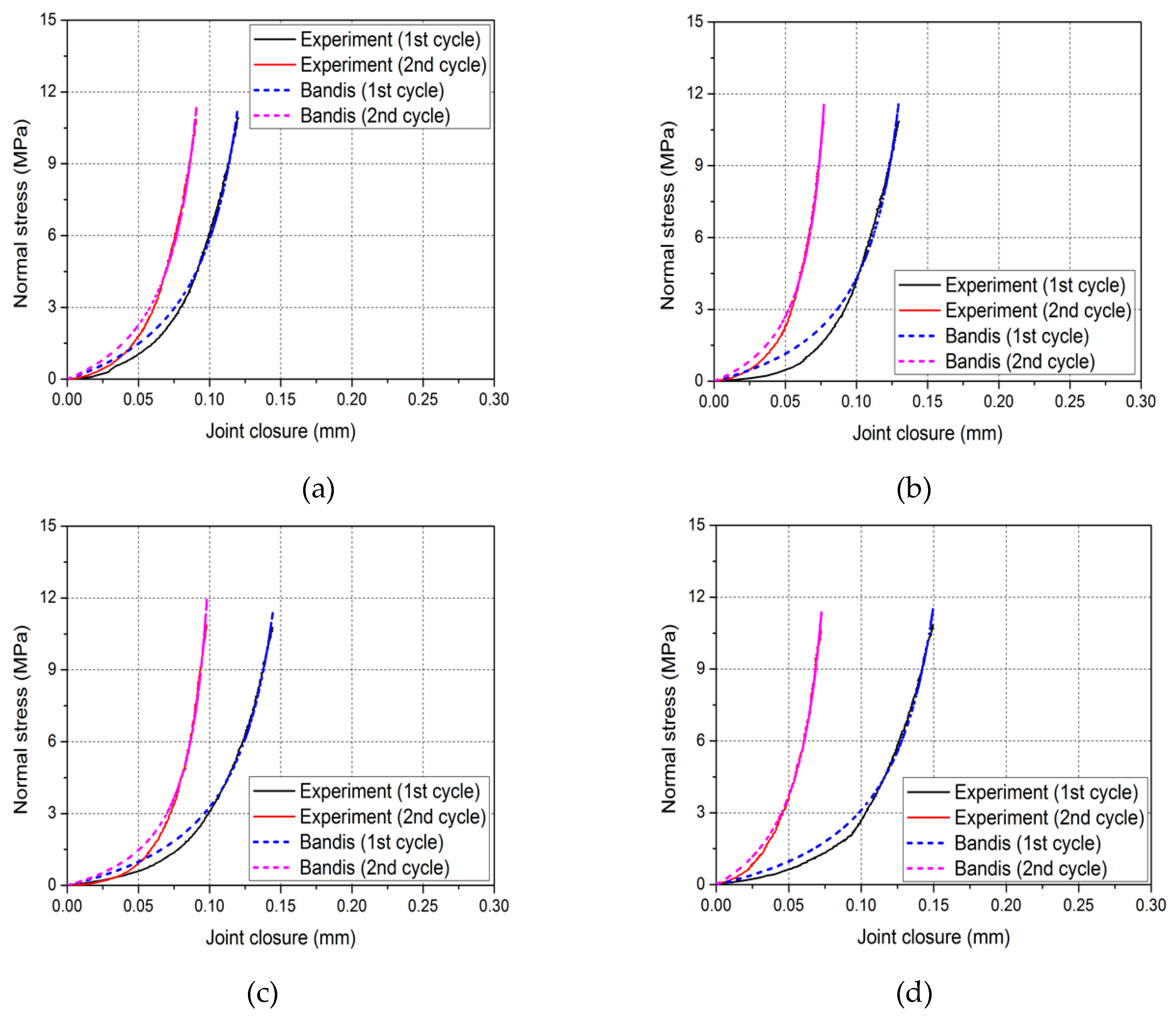
In 1983, Bandis et al. [9] extensively explained behavior of joint under various stress states. Displacement of joint (or joint closure) due to normal stress can be written in Equation (3).

$$\Delta {\delta }_j=\Delta {\delta }_{net}-\Delta {\delta }_i$$

(3)

where $\Delta {\delta }_j$ is the deformation of joint or joint closure, $\Delta {\delta }_{net}$ is the net deformation, and $\Delta {\delta }_i$ is the deformation of intact matrix. Therefore, by subtracting the matrix component of deformation from net deformation, the joint closure can be calculated. The joint closure due to normal stress can be modelled by several equations. Goodman (1976) [34] and Bandis et al. (1983) [9] suggested hyperbolic models, while Brown and Scholz (1986) [35] proposed a logarithm model. Normal compression results of this study were applied to those three models and good agreements were achieved using each of them. Figure 6 shows an example of application to Bandis model, which is presented in Equation (4), showing good agreement especially for normal stress larger than 3 MPa.

$$\sigma {\text{'}}_n=\frac{\Delta {\delta }_j}{a-b\cdot \Delta {\delta }_j}$$

(4)

where $a$ and $b$ are fitting constants.

Overall trends were similar regardless of the roughness. Remarkable nonlinear behavior was observed at the early loading stage in both loading cycles. At the early loading region, the normal displacement greatly increased with the normal stress, then, gradually increased in a linear tendency. At the last loading stage, which corresponded with some part where the applied normal stress was close to the maximum 10 MPa, deviation from the linear tendency was not observed since the maximum applied stress (10 MPa) was not large enough compared with the material strength (48.15 MPa). In the second loading cycle, nonlinear deformation at the early loading stage was smaller than the first. It was the effect of stress hysteresis, specifically the effect of permanent closure. The magnitude of joint closure increased with the increase of roughness. It was understandable that the initial mechanical aperture and its dispersion increased with the roughness (Table 1) so that the normal displacement increased with the roughness as well because there had been more space to be deformed at the beginning.

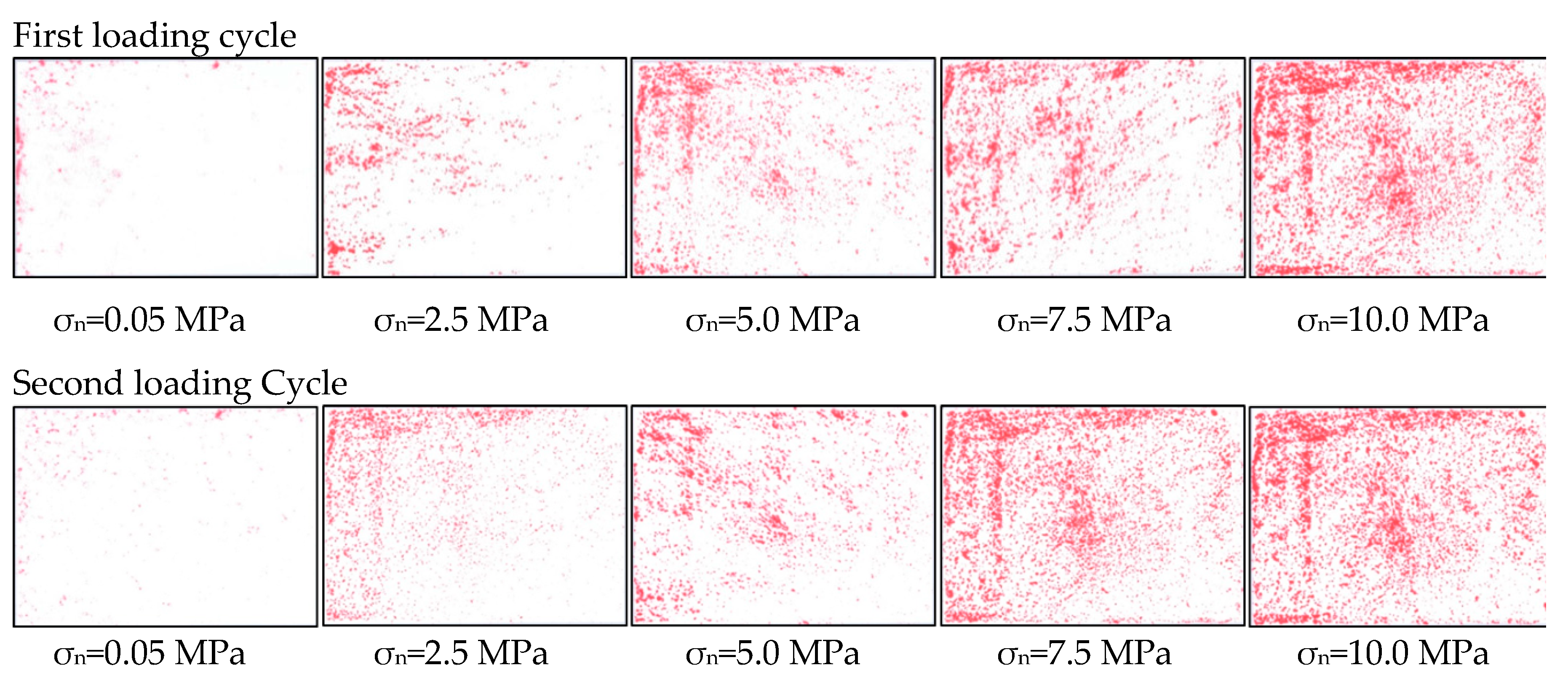
Contact area is the area where the surfaces are in contact, transferring stresses [7]. It exerts great influence on hydromechanical behavior of a joint. In order to measure it in experiments, pressure-sensitive paper was used in this study. It is a two-sheet paper, which is composed of two polyester bases. The one is coated with a layer of micro-encapsulated color forming material and the other is coated with a layer of the color developing material. When pressure is applied to a pair of layers, some parts to which the pressure is applied, i.e., contact area, are painted. Contact area under normal compression was measured in experiments. Applied normal stresses were 0.05, 2.5, 5.0, 7.5, and 10.0 MPa, respectively. Since the paper cannot measure the contact area in real-time and cannot recover its state once color is developed, every test should be paused after reaching target stress and new paper inserted. Figure 7 shows an example of J1 specimen. Size of the paper was 75 mm × 54 mm, same as the joint specimen.

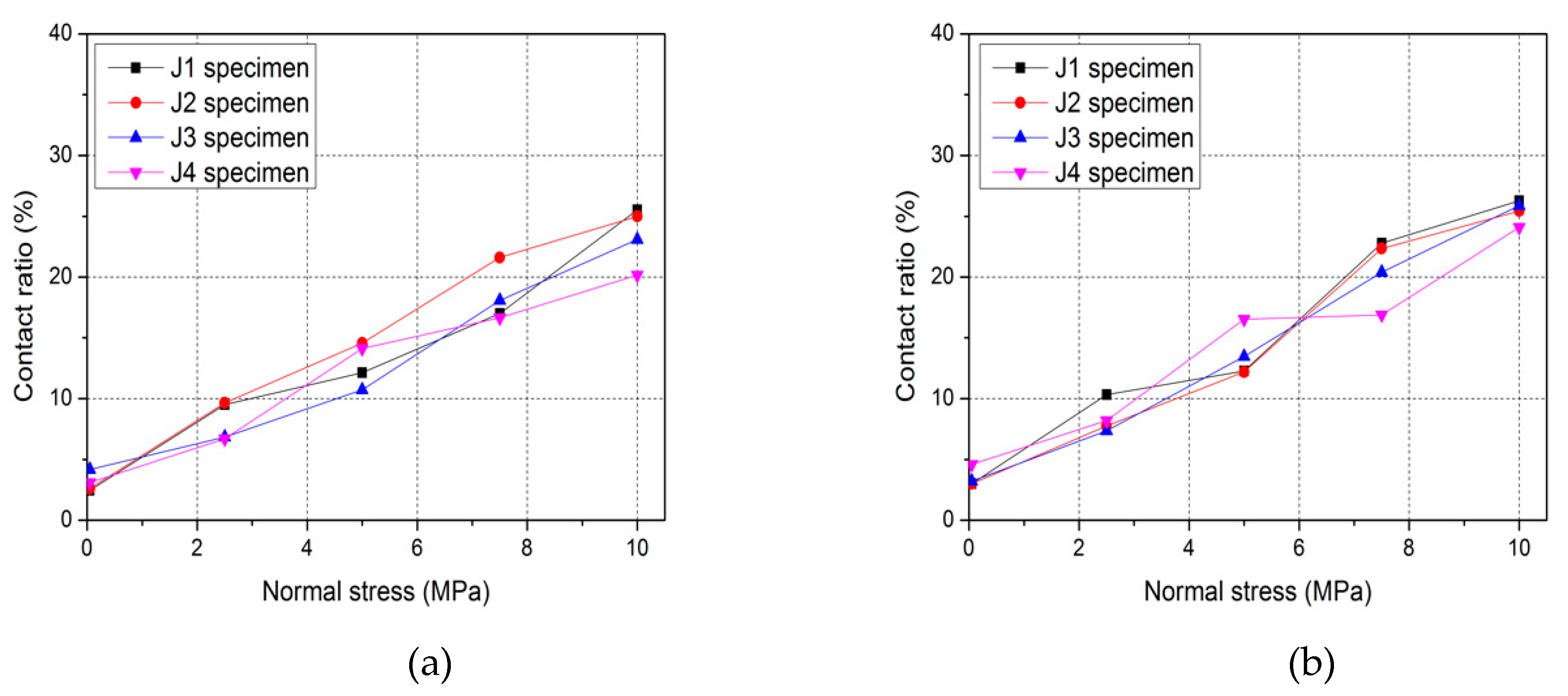
The contact area increased with the increase of normal stress. However, the contact occurred at specific parts even if the stress was increased to 10 MPa so that considerable area remained separated. Overall spatial distribution was similar regardless of loading cycle. However, the contact area in the second cycle was measured slightly larger than the first. In order to analyze it quantitatively, image analyses were conducted. The colored paper was carefully scanned then image files of the scanning were generated. After being imported to analyzing program, the image files were converted into binary images for convenience. Then, the contact area was calculated using the number of total pixels and the number of colored pixels. Results are shown in Figure 8.

As the normal stress increased, the contact area quantitatively increased as well. Under the normal stress of 10 MPa, the maximum contact area was approximately 25% (second loading cycle of J1 specimen), much more parts remained separated. It was similar to the results of Gale (1987) [36] and Pyrak-Nolte et al. (1987) [37]. In most cases, contact area in the second cycle was larger than the first, which was the effect of permanent closure and asperity deformation. The maximum amount of increase due to stress hysteresis was 7.6% (J3 specimen under the normal stress of 7.5 MPa). Under low level of normal stress (especially under 0.05 MPa), the rougher the surface, the larger the contact area was measured. However, this trend became reversed as the stress increased so that J1 specimen had the largest contact area when the stress was 10 MPa.

Mechanical aperture, as well as fracture void, varied due to applied stress. There are two methods capable of calculating the mechanical aperture under specific normal stress. One method is using results of normal compression tests and the other method is back-calculation based on the contact area. In the former method, Equation (5) can be utilized.

$$\begin{gathered} \mathrm{First}\mathrm{loading}\mathrm{cycle}{e}_m=e_{m0}-\Delta {\delta }_j \\ \mathrm{Sec}\mathrm{ond}\mathrm{loading}\mathrm{cycle}{e}_m=(e_{m0}-{\delta }_p)-\Delta {\delta }_j \end{gathered}$$

(5)

where $e_m$ is the mechanical aperture, $e_{m0}$ is the initial mechanical aperture, and ${\delta }_p$ is the permanent closure. The initial mechanical aperture was measured earlier by 3D laser scanner and joint closure values were measured by MTS system in normal compression tests so that the mechanical aperture under specific stress could be calculated.

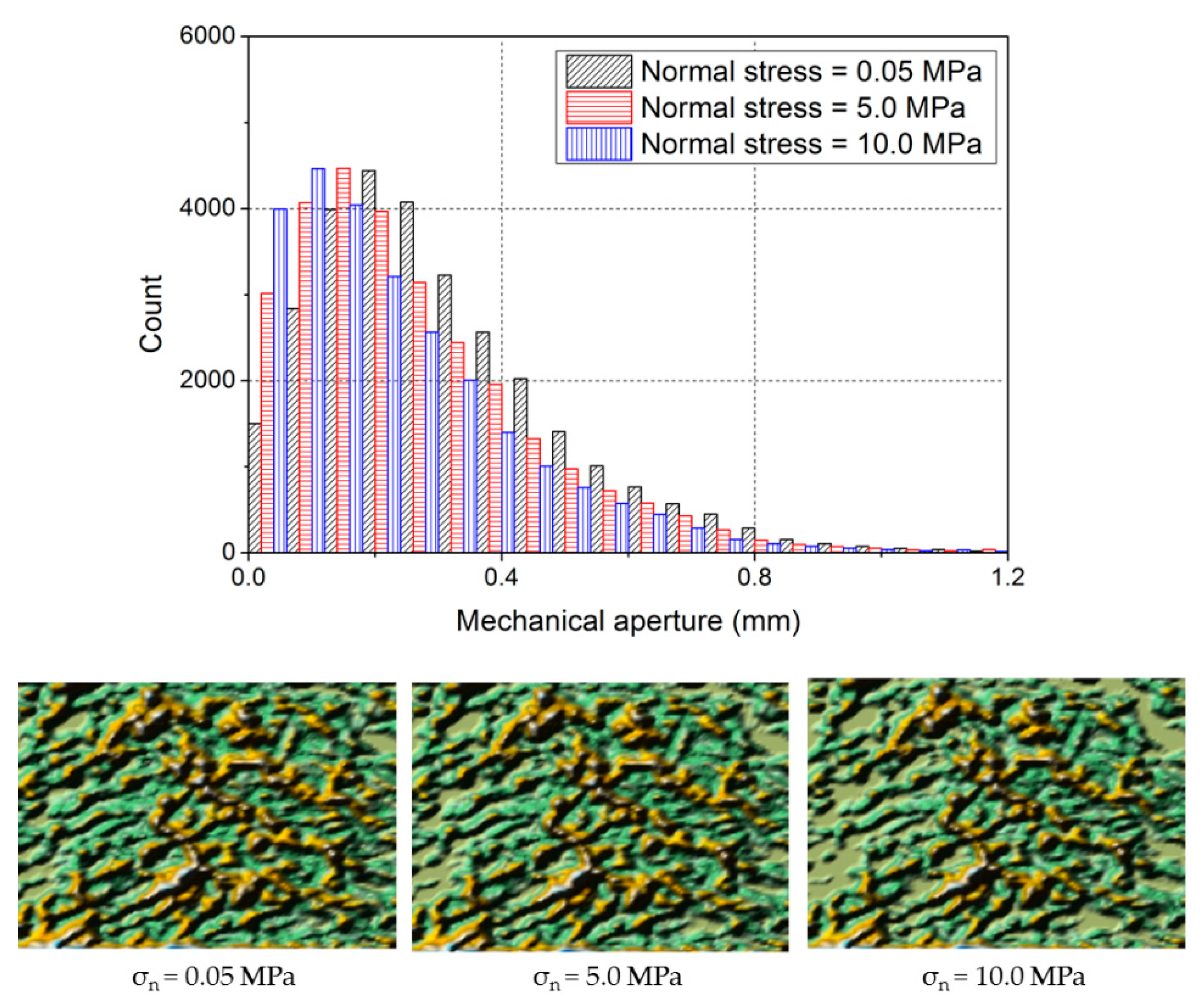
At the same time, back-calculation was possible, since the information about the initial void geometry and the contact area were measured by 3D laser scanning and pressure-sensitive paper, respectively. The back-calculation process was performed as follows. First, scanned coordinates of both upper and lower surfaces were arranged vertically. Then, the upper surface data was translated along downward step-by-step until the percentage of overlapping surface points equaled the measured contact area. When the criterion was met, not only average of the aperture but spatial distribution could be calculated. Figure 9 shows variation of aperture histogram and spatial distribution according to the normal stress, excerpted from J2.

As the normal stress increased, the fracture void was compressed so that the histogram in Figure 9 was shifted toward left. Meanwhile, the spatial distribution in Figure 9 conceptually shows how the aperture distributed in the fracture void and varied by the normal stress. Yellow parts and flat parts in the bottom plot denote the large aperture and contact area, respectively. As the normal stress increased, remarkable change was observed. Flat spaces, which denote the contact area, broadened and void spaces became narrower and smaller, indicating possible channeling effect in flow experiments.

3.3. Hydraulic Characteristics

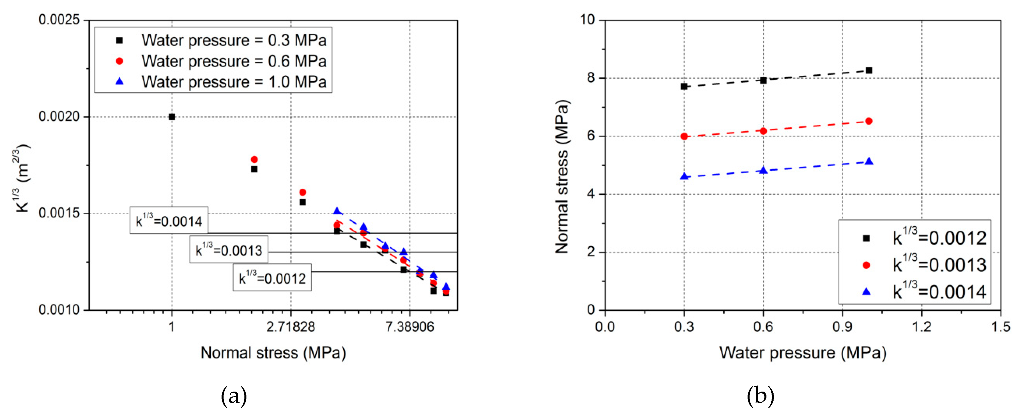
Testing assembly, which included joint specimen and two endcaps, was placed in the triaxial compression chamber. Triaxial unit controlled the normal stress, which was from 1 to 10 MPa with the interval of 1 MPa, and pore pressure unit controlled the water pressure, which was 0.3, 0.6, and 1.0 MPa. Stress hysteresis was also investigated in flow experiments. When the water or pore pressure acts on a medium, stress components of the medium can be expressed in Equation (6).

$$\sigma \text{'}=\sigma -\alpha P_w$$

(6)

where $\sigma \text{'}$ is the effective stress, $P_w$ is the water pressure, and $\alpha$ is the effective stress coefficient, sometimes referred as Biot’s coefficient. Since the normal stress and water pressure were applied step-by-step, the cross-plot method for determining the effective stress coefficient of joint could be applied [38]. Procedures for applying the cross-plot method are briefly described as follows. At first, permeability, more precisely cube root of the permeability, of a joint is calculated by flow tests and is plotted as a function of water pressure at constant normal stress (Figure 10a). Horizontal lines in Figure 10a denote the cross-plotting and make intersecting points. The points are plotted again (Figure 10b) in normal stress-water pressure coordinates system so that the slope of the line in Figure 10b is the effective stress coefficient.

As a result, the joint specimens, i.e., J1, J2, J3, and J4, had 0.80, 0.87, 0.75, and 0.82 of the coefficients, respectively. The coefficients were adopted when calculating the effective stress in following process.

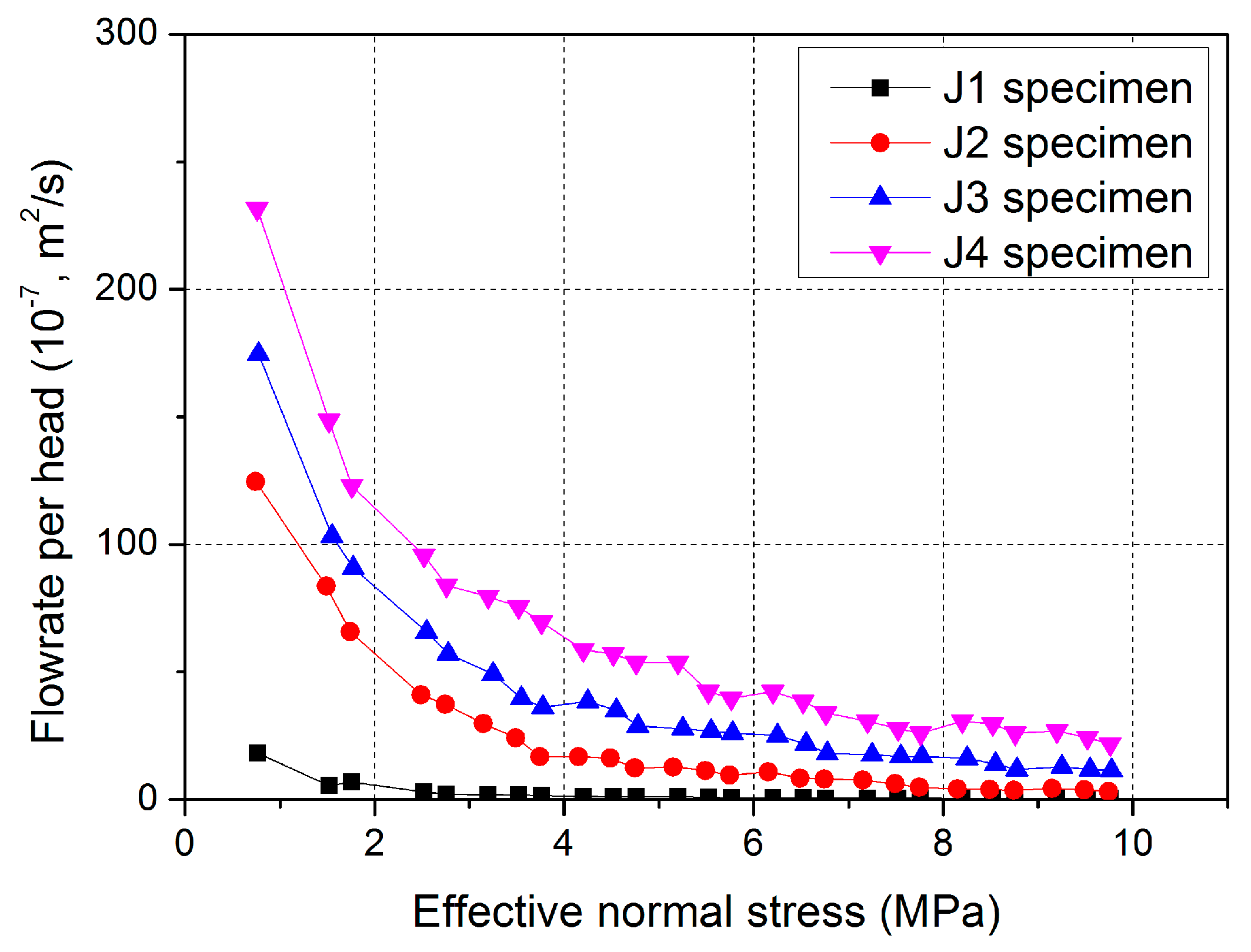
Based on the measured flowrate and applied water pressure, flowrate per unit hydraulic head ($Q/\Delta h$) could be calculated. Figure 11 shows the effect of roughness and effective stress on the flowrate. The results were excerpted from the first loading cycle.

As shown in Figure 11, an increase in effective normal stress made the aperture narrower so that the flowrate decreased. An abrupt decrease at the early loading stage was observed. When comparing the flowrate under 1 MPa and 10 MPa of applied normal stress, J1 specimen showed 54 times of reduction, while J4 showed 11 times of reduction. The effect of roughness is clearly shown in Figure 11. The rougher the joint, the larger flowrate per head was measured, since the rougher joint always had larger aperture value under the same level of normal stress in this study. The same tendencies were found in the second loading cycle in terms of the effect of roughness and normal stress.

If fluid flow through a joint is steady and isothermal, the flowrate per unit hydraulic head in case of straight flow [20] can be written in Equation (7), which is commonly known as cubic law. The law is derived from smooth, parallel, and open plate model.

$$\frac{Q}{\Delta h}=C{e}_h^3=\left(\frac{W}{L}\right)\left(\frac{\rho g}{12\mu }\right)e_h^3$$

(7)

where $e_h$ is the hydraulic (equivalent) aperture, $W$ and $L$ are the width and length of the joint, $g$ is the gravitational acceleration (9.81 $m/s^2$), $\rho$ and $\mu$ are the density and viscosity of the fluid, respectively. Therefore, the hydraulic aperture could be calculated based on the measured flowrate. The width and length of the joint were 54 mm and 75 mm, respectively, and properties of water at 20 °C were applied (approximately 1000 $kg/m^3$ and 1.002 $mPa\cdot s$ for density and viscosity, respectively). Since the mechanical aperture under specific normal stress was already measured, a comparison between the mechanical and corresponding hydraulic apertures could be made, shown for J1 specimen in Figure 12.

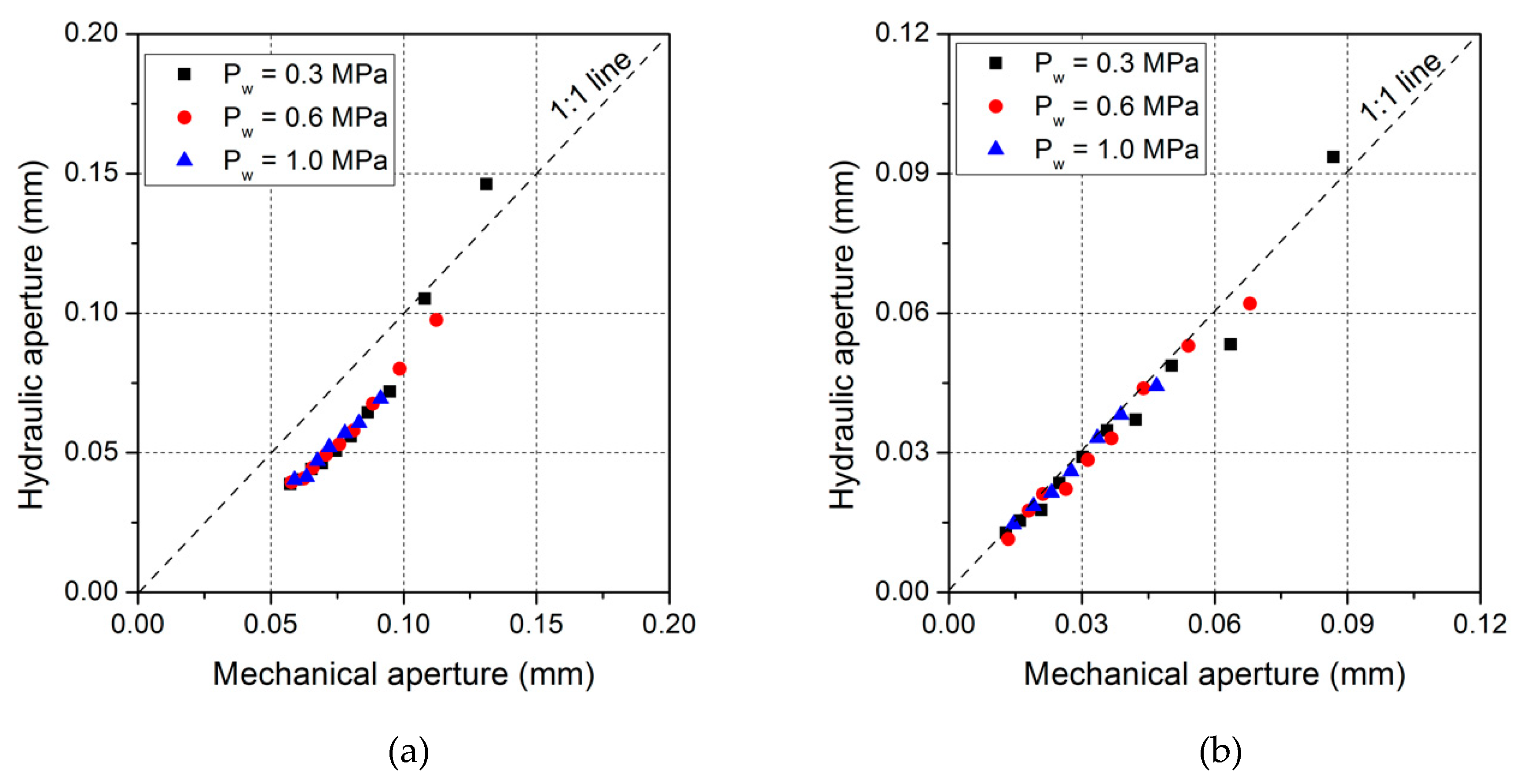
If the two apertures are same, results lay on 1:1 line in Figure 12. It means the cubic law stands, which also indicates ideal joint conditions in Equation (7), i.e., smooth, parallel, and open condition, hold true. However, since it is not the case in real rock joint, deviations from the ideal case are inevitable. This phenomenon is affected by many factors, such as roughness, contact area, tortuosity, and so on. And the further the joint condition from the ideal one, the more deviation is measured. Even though J1 specimens had quite small roughness, deviation from 1:1 line was clearly observed in Figure 12a. A ratio of hydraulic aperture to mechanical aperture ($e_h/e_m$) for J1, J2, J3, and J4 specimen was measured as 0.72, 0.46, 0.39, and 0.29, respectively, on average, which meant the mechanical aperture was always larger than the hydraulic aperture. A few points in Figure 12 were located above the 1:1 line, however, it was reasonable to think that they were caused by systematic error during experiments. Therefore, the effect of roughness on the flow behavior, which impeded overall flow, could be investigated qualitatively and many references reported the same tendency [3,11]. When it comes to the stress hysteresis, Figure 12b showed that the results located much closer to 1:1 line. It could be explained that deformation of asperity due to normal stress and permanent closure made more ideal joint condition so that the experimental discrepancies were narrowed.

4. Discussion

Various studies proposed a relationship between mechanical and hydraulic apertures. By linking the apertures into an equation, predictions for hydraulic behavior of joint were conducted. Among numerous relationships, prediction models suggested by Barton et al. (1985) [19], Zimmerman and Badvarsson (1996) [20], and Matsuki et al. (2006) [39] are listed in

Table 2. Comparison of referenced prediction models.

Authors	Equation
Barton et al. (1985) [19]	(8)
Zimmerman and Bodvarsson (1996) [20]	(9)
Matsuki et al. (2006) [39]	(10)

.

$$e_h=\frac{JR{C}^{2.5}}{{(e_m/e_h)}^2}$$

(8)

$${\left(\frac{e_h}{e_m}\right)}^3=\left[1-1.5{\left(\frac{{\sigma }_m}{e_m}\right)}^2\right](1-2c)$$

(9)

$${\left(\frac{e_h}{e_m}\right)}^3=\left[1-\frac{1.13}{1+0.191{(2e_m/{\sigma }_{m0})}^{1.93}}\right]$$

(10)

where ${\sigma }_m$ and $c$ in Equation (9) are the standard deviation of mechanical aperture and the contact ratio, respectively, and ${\sigma }_{m0}$ in Equation (10) is the standard deviation of initial mechanical aperture. They have their own strength and shortcomings. Equation (8) was a rough empirical model derived from numerous data results. It is widely used, since it has relatively simple form and $JRC$ in the equation. However, in some cases, it loses its applicability or shows estimation error especially when joints are under shear behavior. Equation (9) considers not only roughness effect, the first bracket in Equation (9), but also contact effect. Equation (10) was derived from numerical simulations.

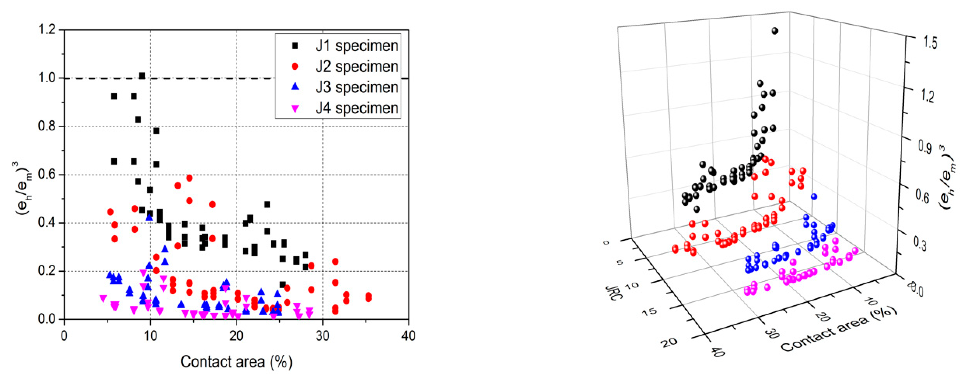
In this study, a prediction model for $e_h/e_m$ was proposed based on the experimental results described above. It was thought that a prediction model with one parameter was not sufficient to represent the experimental results. Therefore, $JRC$ and contact area ($c$) were selected as independent variables. All relevant results were arranged and calculated again, and Figure 13 shows a relationship between ${(e_h/e_m)}^3$ and those two variables.

As described in Section 3, ${(e_h/e_m)}^3$ decreased with the increase of $JRC$ and $c$, which indicated the effect of roughness and contact area hampered the fluid flow, causing the discrepancy between those two apertures to become larger. Correlation analyses between ${(e_h/e_m)}^3$ and $JRC$, $c$ were conducted and the results are shown in

Table 3. Correlation analyses between variables.

		$c$	$JRC$	${(e_h/e_m)}^3$
$c$	Pearson correlation	1
	Sig. (2-tailed)	-
$JRC$	Pearson correlation	−0.096	1
	Sig. (2-tailed)	0.175	-
${(e_h/e_m)}^3$	Pearson correlation	−0.345 **	−0.693 **	1
	Sig. (2-tailed)	0.000	0.000	-

** Correlation is significant at the 0.01 level (2-tailed).

. Bivariate analyses including all three variables were performed and the results showed that both independent variables, i.e., $JRC$ and $c$, had negative correlations with ${(e_h/e_m)}^3$. As mentioned before, ${(e_h/e_m)}^3$ decreased when the independent variables increased. $JRC$ and $c$ were found to be independent of each other, showing weak negative relationships, but statistically meaningless within 5% of significant level.

Based on the experimental results, Equation (11) was proposed. In order to consider the effects of independent variables, negative exponential functions were adopted. At the same time, coefficients of the regression model were determined considering the fact that ${(e_h/e_m)}^3$ should be in unity when both $JRC$ and $c$ equaled zero, which means flat and open joint so that the ideal cubic law condition is achieved.

$${\left(\frac{e_h}{e_m}\right)}^3=\exp (-0.0462c)\times {(0.8864)}^{JRC}$$

(11)

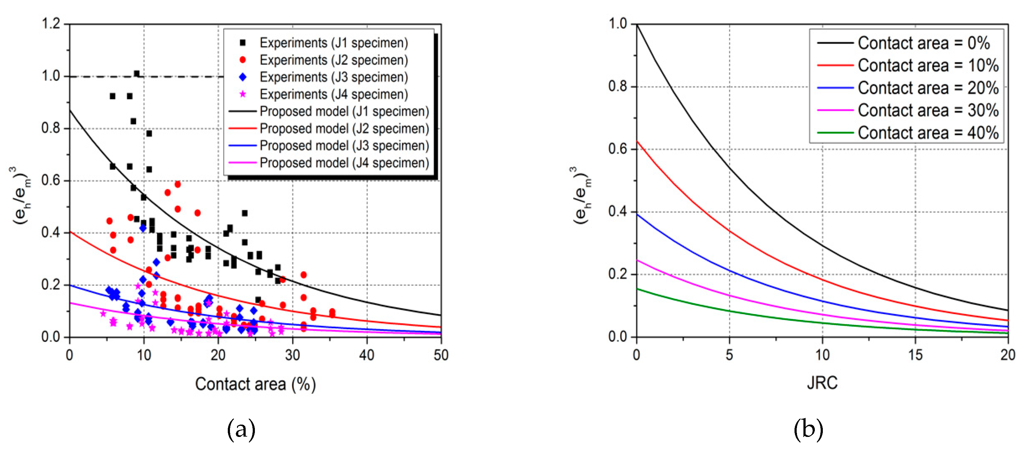
Figure 14 shows application of the proposed model to experimental results and its variation according to the $JRC$ and $c$. As it can be seen in Figure 14a, the proposed prediction model agreed relatively with the experimental results. Adjusted r-square of three-dimensional fitting was 0.74, which is thought to be acceptable in engineering viewpoint. At the same time, root mean square error (RMSE) between the measured and predicted values was calculated as 0.1078.

Variations of the proposed model were investigated. Figure 14b shows the variation according to $JRC$ with fixed contact area of 0, 10, 20, 30, and 40%. In the case of $JRC$ equaling zero, which means a flat joint, the contact area should be 0 or 100, which corresponds with ${(e_h/e_m)}^3$ equaling 1 or 0. However, this case could not be modelled in this study. Based on the results of $JRC$=1, ${(e_h/e_m)}^3$ decreased to 33% and 10% when $JRC$ increased to 10 and 20, respectively. It is noteworthy that the experimental results were obtained from a relatively wide range of $JRC$. On the other hand, the measured contact area in experiments had the range of 4~35%. Therefore, one needs to be cautious when a contact area larger than 35% is in consideration.

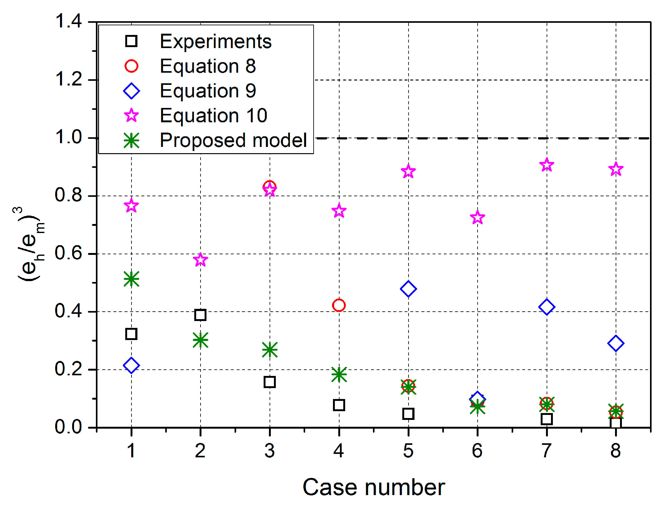
The performance of the proposed model was compared with referenced models. Equations (8)–(10) were applied to the experimental results in this study. Among several results, eight cases were excerpted and applied.

Table 4. Comparison between the referenced models and proposed model.

		Experiment	Equation (8)	Equation (9)	Equation (10)	Proposed
J1	Case1	0.3327	273.2437	0.2149	0.7658	0.5136
	Case2	0.3789	158.0083	−0.1617	0.5782	0.3030
J2	Case3	0.1565	0.8306	−0.1354	0.8195	0.2692
	Case4	0.0771	0.4223	−0.4362	0.7474	0.1839
J3	Case5	0.0467	0.1443	0.4792	0.8837	0.1402
	Case6	0.0920	0.0907	0.0981	0.7246	0.0731
J4	Case7	0.0289	0.0837	0.4162	0.9060	0.0802
	Case8	0.0147	0.0533	0.2914	0.8918	0.0570

and Figure 15 show measured ${(e_h/e_m)}^3$ values in experiments and predicted values by Equations (8)–(10), along with predicted values by the proposed model in this study.

In Barton model (Equation (8)), Cases 1 and 2 produced ${(e_h/e_m)}^3$ values that highly exceeded 1, which was not acceptable. This is because of the inherent limitation of the model, which is not capable of applying to joints with small roughness. Results of Cases 3 and 4 were less than 1, however, they still showed larger discrepancies compared with the experimental results. From Cases 5 to 8, the results became much closer to the experimental results, therefore, it is thought that Barton model is suitable for joints with relatively large roughness. In some cases, Zimmerman model (Equation (9)) derived negative ${(e_h/e_m)}^3$ values. This is because the first term in right side of Equation (9), which includes a ratio of standard deviation to average of mechanical aperture. By definition, the terms larger than approximately 0.8165 gave negative results. However, sometimes this could be found in experiments and corresponds to joints under high normal stress or highly weathered joints [3,39]. Equation (10) always produced ${(e_h/e_m)}^3$ values less than 1, however, the predicted values were relatively larger than the experiments, which was thought to be the effect of initial mechanical aperture in the equation.

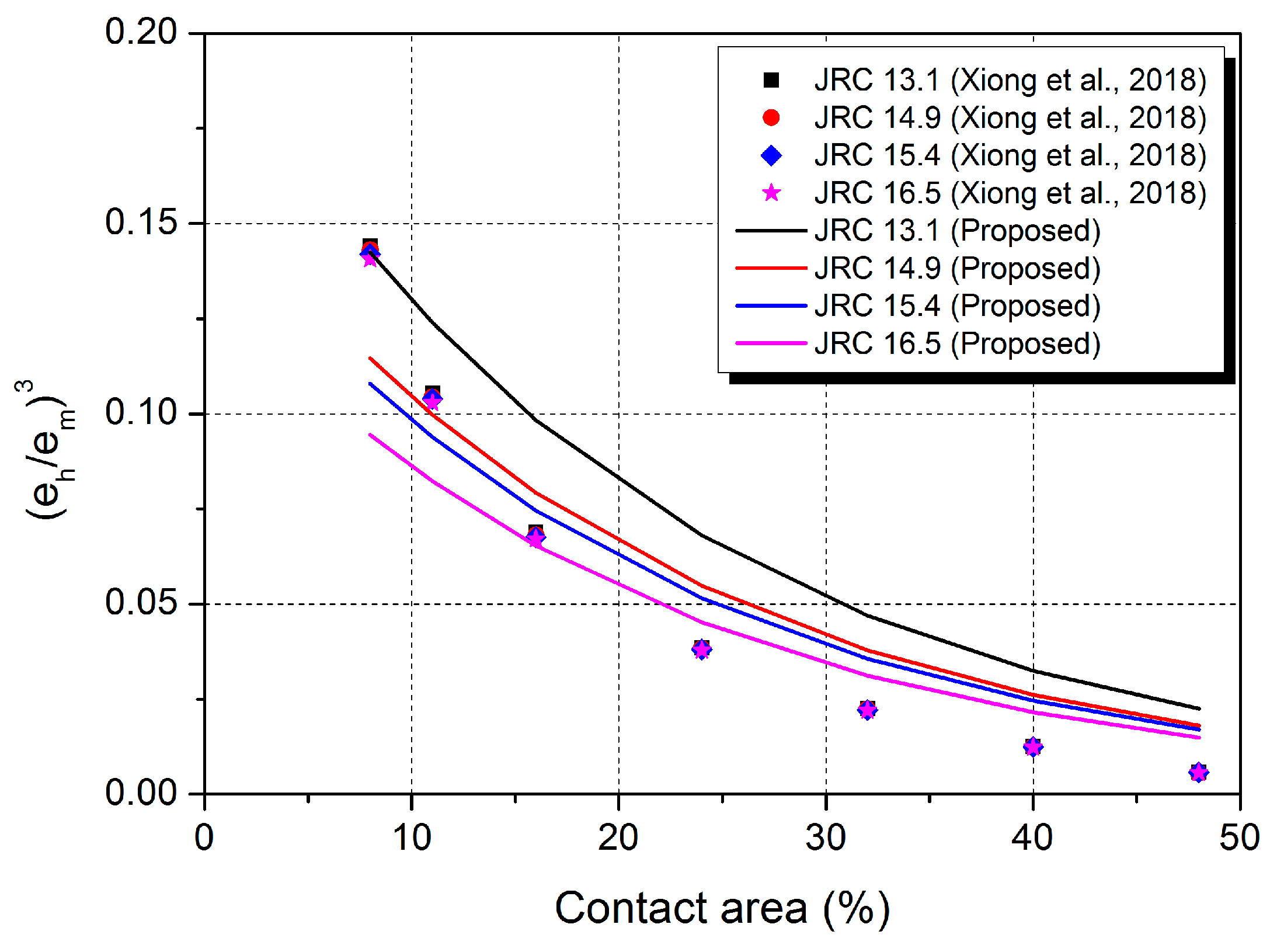
For more verification, numerical simulation results by Xiong et al. (2018) [21] were referenced. They tested granite joint specimens and measured the information of fracture void using 3D laser scanner and conducted numerical simulations. Based on the simulation results, they suggested a relationship as a function of contact area and fractal dimension. Since it provided comparable results, such as mechanical aperture, roughness, and contact area, their results were excerpted and applied to Equation (11). In order to make direct comparison, the fractal dimension in Reference [21] was converted into $JRC$. Figure 16 shows the verification result.

As shown in Figure 16, overall trends of the two models were similar to each other. ${(e_h/e_m)}^3$ decreased with the increase of $JRC$ and with the increase of contact area. Some discrepancies were observed between them. However, the amount was quite smaller than the previous comparison. The Xiong model showed clear variation according to the contact area, but on the other hand, variation due to roughness was not significant. This was because their granite specimens had similar roughness level ($JRC$ of 13~16).

Comparisons with referenced prediction models above showed that a few models could not be applied in some cases or show significant discrepancies. A couple of explanations could be deduced. First, those prediction models were derived from a specific range of geometric properties, which cannot be extended to wider cases. The matching state of the joint also affects the hydraulic features, but is not properly considered in some models. The proposed prediction model in this study considered a relatively wide range of roughness and, at the same time, consideration on the matching state was taken at some degree since the contact area was included in the model. Meanwhile, the proposed model also has a couple of limitations. First, the prediction model was constructed based on the limited data in terms of the contact area. $JRC$ was distributed relatively evenly within the range of 0~20, while the contact area was 4~35%. Therefore, it could not guarantee its applicability when the input data outlays the range, especially in a contact area larger than 35%.

Analyses on hydromechanical characteristics in rock mass scale, such as discreet fracture network (DFN), should be conducted based on the accurate understanding of a joint. Several features of a joint are required in DFN, and among them, aperture is a critical parameter [40]. Distribution of mechanical aperture and its relationship with hydraulic aperture should be taken into account when building DFN models. In 2016, Luo et al. stated that most of the previous DFN studies assumed identical hydraulic and mechanical apertures in joint distribution for simplicity. In their study, remarkable discrepancies in macroscopic flowrate were observed depending on the selected relationship between apertures [41]. It indicated significant importance on prediction of hydraulic aperture so that emphasis could be made regarding understanding on characteristics of a joint.

5. Conclusions

The hydromechanical characteristics of a joint are affected by many joint parameters, such as roughness, aperture, contact area, stiffness, etc. Among them, the effects of roughness and aperture on the features are widely studied by various approaches. In many cases, artificial joint specimens are prepared to carry out laboratory experiments. However, controlling the roughness in experiments requires excessive efforts, since the specimens are often created mechanically. Therefore, some experimental works were derived from limited testing conditions in terms of the geometric properties of joint. In this study, the limitation was overcome to some extent using 3D printing technique. A fractal theory, specifically the random midpoint displacement method, was adopted to generate three-dimensional joint surfaces. By manipulating the input parameters of the method, the roughness of joint surfaces could be controlled in a quantitative manner.

Throughout the experimental works, four different joint specimens (J1, J2, J3, and J4) were prepared, which had $JRC$ of 1.12, 7.32, 13.07, and 16.47, respectively. Therefore, in terms of $JRC$, the geometric condition of this study was distributed relatively evenly within the range of 0~20. Mechanical aperture and its distribution were calculated based on the scanned data as well. By adopting superposition method, initial mechanical aperture of the four joint specimens was calculated and as a result, it could be found that $JRC$ and the initial mechanical aperture had positive correlation.

Normal compression tests were conducted so as to obtain joint displacement under specific stress. The maximum normal stress was 10 MPa, which corresponded with vertical in-situ stress of 400 m. As a result, the overall behavior agreed well with previous researches being simulated successfully by referenced relationships. The larger the roughness, the larger joint displacement was measured under normal compression. Variation of contact area was measured by pressure-sensitive paper. Effects of normal stress and stress hysteresis were investigated by image analyses of dyed paper, however quantitative relationship with roughness could not be found. Not only the average of aperture under normal stress, but also the spatial distribution was calculated by parallel translation of the joint surface.

Flow tests under normal compression were performed under maximum 1 MPa of water pressure. As the normal stress increased, flowrate per unit hydraulic head decreased since the aperture was compressed. Also, the rougher the surface, the larger flowrate was measured. For instance, J4 specimen showed 64 times higher flowrate than J1 specimen under 10 MPa of normal stress. Hydraulic aperture can be calculated with the assumption of cubic law. Then, comparison between the mechanical aperture and hydraulic aperture could be made. In a rough joint, deviation from the ideal condition of cubic laws are inevitable, since many factors affect fluid flow, such as roughness, contact area, channeling, etc. The mechanical and hydraulic apertures had positive correlation, however, more deviations were observed when the roughness increased.

Based on the experimental results, a prediction model for the hydraulic aperture was proposed. It was found that a model with single variable showed insufficient prediction capability so that the model was constructed as a function of roughness and contact area. As a result, ${(e_h/e_m)}^3$ could be expressed by those two variables having negative correlations. The effect of contact area was expressed as a negative exponential function and the effect of roughness was as an exponential function that had roughness as an exponent. The model showed an adjusted r-square of 0.74 and acceptable prediction performance comparing with several referenced models.

References

- Makurat, A.; Barton, N.; Rad, N.S.; Bandis, S. Joint conductivity variation due to normal and shear deformation. In Proceedings of the International Symposium on Rock Joints, Leon, Norway, 4–6 June 1990; pp. 535–540. [Google Scholar]
- Esaki, T.; Du, S.; Mitani, Y.; Ikusada, K.; Jing, L. Development of a shear-flow test apparatus and determination of coupled properties for a single rock joint. Int. J. Rock Mech. Min. Sci. 1999, 36, 641–650. [Google Scholar] [CrossRef]
- Lee, H.S.; Cho, T.F. Hydraulic characteristics of rough fractures in linear flow under normal and shear load. Rock Mech. Rock Eng. 2002, 35, 299–318. [Google Scholar] [CrossRef]
- Hakami, E.; Larsson, E. Aperture measurement and flow experiments on a single natural fracture. Int. J. Rock Mech. Min. Sci. 1996, 33, 395–404. [Google Scholar] [CrossRef]
- Min, K.B.; Rutqvist, J.; Elsworth, D. Chemically and mechanically mediated influence on the transport and mechanical characteristics of rock fractures. Int. J. Rock Mech. Min. Sci. 2009, 46, 80–89. [Google Scholar] [CrossRef]
- Brown, S. Fluid flow through rock joints: The effect of surface roughness. J. Geophys. Res. Solid Earth 1987, 92, 1337–1347. [Google Scholar] [CrossRef]
- Hakami, E. Aperture Distribution of Rock Fractures. Ph.D. Thesis, Division of Engineering Geology, Royal Institute of Technology, Stockholm, Sweden, 1995. [Google Scholar]
- Olsson, R.; Barton, N. An improved model for hydromechanical coupling during shearing of rock joints. Int. J. Rock Mech. Min. Sci. 2001, 38, 317–329. [Google Scholar] [CrossRef]
- Bandis, S.; Lumsden, A.; Barton, N. Fundamentals of rock joint deformation. Int. J. Rock Mech. Min. Sci. 1983, 20, 249–268. [Google Scholar] [CrossRef]
- Pyrak-Nolte, L.J.; Morris, J.P. Single fractures under normal stress: The relation between fracture specific stiffness and fluid flow. Int. J. Rock Mech. Min. Sci. 2000, 37, 245–262. [Google Scholar] [CrossRef]
- Zhao, J.; Brown, E. Hydro-thermo-mechanical properties of joints in the Carnmenellis granite. Q. J. Eng. Geol. 1992, 25, 279–290. [Google Scholar] [CrossRef]
- Park, J.; Song, J. Numerical method for the determination of contact areas of a rock joint under normal and shear loads. Int. J. Rock Mech. Min. Sci. 2013, 58, 8–22. [Google Scholar] [CrossRef]
- Singh, K.K.; Singh, D.N.; Ranjith, P.G. Laboratory simulation of flow through single fractured granite. Rock Mech. Rock Eng. 2015, 48, 987–1000. [Google Scholar] [CrossRef]
- Scesi, L.; Gattinoni, P. Roughness control on hydraulic conductivity in fractured rocks. Hydrogeol. J. 2007, 15, 201–211. [Google Scholar] [CrossRef]
- Koyama, T.; Li, B.; Jiang, Y.; Jing, L. Numerical modelling of fluid flow tests in a rock fracture with a special algorithm for contact areas. Comput. Geotech. 2009, 36, 291–303. [Google Scholar] [CrossRef] [Green Version]
- Xiong, X.; Li, B.; Jiang, Y.; Koyama, T.; Zhang, C. Experimental and numerical study of the geometrical and hydraulic characteristics of a single rock fracture during shear. Int. J. Rock Mech. Min. Sci. 2011, 48, 1292–1302. [Google Scholar] [CrossRef]
- Yeo, I.; Freitas, M.; Zimmerman, R. Effect of shear displacement on the aperture and permeability of a rock facture. Int. J. Rock Mech. Min. Sci. 1998, 35, 1051–1070. [Google Scholar] [CrossRef]
- Gentier, S.; Riss, J.; Archambault, G.; Flamand, R.; Hopkins, D. Influence of fracture geometry on shear behavior. Int. J. Rock Mech. Min. Sci. 2000, 37, 161–174. [Google Scholar] [CrossRef]
- Barton, N.; Bandis, S.; Bakhtar, K. Strength, deformation and conductivity coupling of rock joints. Int. J. Rock Mech. Min. Sci. Abstr. 1985, 22, 121–140. [Google Scholar] [CrossRef]
- Zimmerman, R.; Bodvarsson, G. Hydraulic conductivity of rock fractures. Transp. Porous Media 1996, 23, 1–30. [Google Scholar] [CrossRef]
- Xiong, F.; Jiang, Q.; Chen, M. Numerical investigation on hydraulic properties of artificially-splitting granite fractures during normal and shear deformations. Geofluid 2018, 1–16. [Google Scholar] [CrossRef]
- Raja, J.; Radhakrishnan, V. Analysis and synthesis of surface profiles using Fourier series. Int. J. Mach. Tool Des. Res. 1977, 17, 245–251. [Google Scholar] [CrossRef]
- Patir, N. A numerical procedure for random generation of rough surfaces. Wear 1978, 47, 263–277. [Google Scholar] [CrossRef]
- Xie, H. Fractals in Rock Mechanics; Balkema: Rotterdam, The Netherlands, 1993; ISBN 9054101334. [Google Scholar]
- Choi, S.; Lee, S.; Jeong, H.; Jeon, S. Development of a new method for quantitative generation of an artificial joint specimen with specific geometric properties. Sustainability 2019, 11, 373. [Google Scholar] [CrossRef]
- Barton, N.; Choubey, V. The shear strength of rock joints in theory and practices. Rock Mech. Rock Eng. 1977, 10, 1–54. [Google Scholar] [CrossRef]
- Ulusay, R.; Hudson, J.A. The Complete ISRM Suggested Methods for Rock Characterization, Testing and Monitoring: 1974–2006; ISRM Commission on Testing Method: Ankara, Turkey, 2007; ISBN 9789759367541. [Google Scholar]
- Tse, R.; Cruden, D. Estimating joint roughness coefficients. Int. J. Rock Mech. Min. Sci. Abstr. 1979, 16, 303–307. [Google Scholar] [CrossRef]
- Grasselli, G.; Egger, P. Constitutive law for the shear strength of rock joints based on three-dimensional surface parameters. Int. J. Rock Mech. Min. Sci. 2003, 40, 25–40. [Google Scholar] [CrossRef]
- Park, J.; Lee, Y.; Song, J.; Choi, B. A constitutive model for shear behavior of rock joints based on three-dimensional quantification of joint roughness. Rock Mech. Rock Eng. 2013, 46, 1513–1537. [Google Scholar] [CrossRef]
- Esaki, T.; Du, S.; Jiang, Y.; Wada, Y.; Mitani, Y. Relation between mechanical and hydraulic apertures during shear-flow coupling test. In Proceedings of the 10th Japan Symposium on Rock Mechanics, Osaka, Japan, 22–23 January 1998; pp. 91–96. [Google Scholar]
- Iwano, M.; Einstein, H. Stochastic analysis of surface roughness, aperture and flow in a single fracture. In Proceedings of the EUROCK, Lisbon, Portugal, 21–24 June 1993; pp. 135–141. [Google Scholar]
- Riss, J.; Gentier, S.; Sirieix, C.; Archambault, G.; Flamand, R. Degradation characteristics of sheared joint wall surface morphology. In Proceedings of the 2nd North America Rock Mechanics Symposium, Montreal, QC, Canada, 19–21 June 1996; pp. 1343–1349, ISBN 905410838X. [Google Scholar]
- Goodman, R. Method of Geological Engineering in Discontinuous Rocks; West Publishing: New York, NY, USA, 1976; ISBN 0829900667. [Google Scholar]
- Brown, S.; Scholz, C. Closure of rock joints. J. Geophys. Res. Solid Earth 1986, 91, 4939–4948. [Google Scholar] [CrossRef]
- Gale, J. Comparison of coupled fracture deformation and fluid flow models with direct measurements of fracture pore structure and stress-flow properties. In Proceedings of the 28th US Symposium on Rock Mechanics, Tucson, AZ, USA, 29 June–1 July 1987; pp. 1213–1222. [Google Scholar]
- Pyrak-Nolte, L.; Myer, L.; Cook, N.; Witherspoon, P. Hydraulic and mechanical properties of natural fractures in low-permeability rock. In Proceedings of the 6th ISRM Congress, Montreal, QC, Canada, 30 August–3 September 1987; pp. 225–231. [Google Scholar]
- Walsh, J. Effect of pore pressure and confining pressure on fracture permeability. Int. J. Rock Mech. Min. Sci. Abstr. 1981, 18, 429–435. [Google Scholar] [CrossRef]
- Matsuki, K.; Chida, Y.; Sakaguchi, K.; Glover, P. Size effect on aperture and permeability of a fracture as estimated in large synthetic fractures. Int. J. Rock Mech. Min. Sci. 2006, 43, 726–755. [Google Scholar] [CrossRef]
- Bang, S.H.; Jeon, S.; Kwon, S. Modelling the hydraulic properties of a fractured rock mass at KAERI underground research tunnel by three-dimensional discreet fracture network. In Proceedings of the 7th Asian Rock Mechanics Symposium, Seoul, Korea, 15–19 October 2012; pp. 905–913. [Google Scholar]
- Luo, S.; Zhao, Z.; Peng, H.; Pu, H. The role of fracture surface roughness in macroscopic fluid flow and heat transfer in fractured rocks. Int. J. Rock Mech. Min. Sci. 2016, 87, 29–38. [Google Scholar] [CrossRef]
Figure 1.
Printed joint specimens following the random midpoint displacement method and their 3D models (after Reference [25]).
Figure 2.
A picture of molding assembly (cylindrical molding frames, end plugs with top inlets, and aluminum casting molds in red box) and its computer-aided design (CAD) drawing.
Figure 3.
Experimental setup; (a) overall experimental setup and (b) in-vessel test assembly including joint specimen with the endcaps.
Figure 4.
Schematic diagram for determining joint roughness; (a) three-dimensional plot of a joint and (b) x-z profiles for three y-values as shown in (a) (after Reference [25]).
Figure 5.
Histogram of geometric properties; (a) and (b) initial mechanical aperture (results of J4 specimen as an example).
Figure 6.
Application of normal compression results to model of Reference [9]; (a) J1 specimen, (b) J2 specimen, (c) J3 specimen, and (d) J4 specimen.
Figure 7.
Variation of contact area (marked in red) of J1 specimen at different loading cycles and different normal stresses.
Figure 8.
Results of image analyses on contact area (percentile of the number of colored pixels over total pixels; (a) results of the first loading cycle and (b) results of the second loading cycle.
Figure 9.
Variation of aperture distribution according to normal stress (results of J2 specimen as an example).
Figure 10.
Cross-plot method for determining the effective stress coefficient (results of J3 specimen as an example); (a) relationship between normal stress-permeability, and (b) relationship between water pressure-normal stress (cross-plot results of (a))
Figure 11.
Variation of flowrate per head according to the roughness and effective normal stress (in the first loading cycle).
Figure 12.
Comparison between mechanical and hydraulic aperture under normal stress; (a) results of the first loading cycle and (b) results of the second loading cycle (results of J1 specimen as an example).
Figure 13.
Relationship between and two independent variables.
Figure 14.
Evaluation of the proposed model; (a) application of the proposed model to experimental results and (b) variation of the model according to the variables.
Figure 15.
Comparison between the referenced models and proposed model.
Figure 16.
Verification of the proposed model by comparing with referenced data.