Evaluating China’s Air Pollution Control Policy with Extended AQI Indicator System: Example of the Beijing-Tianjin-Hebei Region


1
School of Information Management and Engineering, Fintech Research Institute, Shanghai University of Finance and Economics, Shanghai 200433, China
2
Business School, University of Shanghai for Science and Technology, Shanghai 200093, China
*
Author to whom correspondence should be addressed.
†
Guanghui Yuan and Weixin Yang are joint first authors. They contributed equally to this paper.
Sustainability 2019, 11(3), 939; https://doi.org/10.3390/su11030939
Submission received: 14 January 2019
/
Revised: 2 February 2019
/
Accepted: 7 February 2019
/
Published: 12 February 2019
(This article belongs to the Special Issue Air Quality Assessment Standards and Sustainable Development in Developing Countries)
Abstract
:This paper calculated and evaluated the air quality of 13 cities in China’s Beijing-Tianjin-Hebei (BTH) region from February 2015 to January 2018 based on the extended AQI (Air Quality Index) Indicator System. By capturing the heterogeneous information in major pollutant indicators and the standardization process, we depicted the important effect of other relevant features of pollutant indicators beyond single-point data. Based on that, we further calculated the assessment value of the air quality of different cities in the BTH region by using the Collaborative Filtering Backward Cloud Model to construct differentiated weights of different indicators. With help of the Back Propagation (BP) Neutral Network, we simulated the effect of the pollution control policies of the Chinese government targeting air pollution since March 2016. Our conclusion is: the pollution control policies have improved the air quality of Beijing by 55.74%, and improved the air quality of Tianjin by 34.38%; while the migration of polluting enterprises from Beijing and Tianjin has caused different changes in air quality in different cities of Hebei province—we saw air quality deterioration by 58.60% and 38.68% in Shijiazhuang and Handan city respectively.
1. Introduction
Among the environmental challenges China is facing now, air pollution is one of the key issues that draw the attention of academic circles [1,2,3,4]. In order to scientifically measure air quality and better prevent and control air pollution, China has officially launched the Technical Regulation on Ambient Air Quality Index (on trial) (HJ 633-2012) in 2016 [5].
Air pollution refers to the circumstances where the concentration of certain substances in the atmosphere reaches a certain level that it can harm the ecosystem as well as humans and other species living in it, and threaten the survival of human beings [6]. Currently, the pollutants that China has covered in regular monitor and air quality evaluation include sulfur dioxide (SO2), nitrogen dioxide (NO2), carbon monoxide (CO), inhalable particles (PM10 and PM2.5), and ozone (O3) [5,7]. Above pollutants all cause serious threats to the sustainable development and health of human beings.
According to the two National Standards on Air Quality Measurement published by the Chinese Ministry of Environmental Protection on 29 February 2012—Ambient air quality standards (GB 3095-2012) and Technical Regulation on Ambient Air Quality Index (on trial) (HJ 633-2012)—that became effective on January 1st, 2016, the air quality measurement of China mainly relies on the calculation of AQI (Air Quality Index), with the method of [5]:
• First, calculate the Individual Air Quality Index of certain pollutant ():
In equation above, represents the mass concentration of pollutant P; is the higher threshold of pollutant concentration near corresponding to specified IAQI (Individual Air Quality Index) regulated by government policy; is the lower threshold of pollutant concentration near regulated by government; is the corresponding IAQI to ; while is the corresponding IAQI to .
• Then, take the largest number from all to calculate the :
Nevertheless, there are some issues to be further discussed in above calculation method:
(1) The final AQI only reflects one pollutant—only the pollutant with the highest . Although it is further defined in “AQI Technical Specifications (Trial Use)” that “when AQI is above 50, the pollutant with the highest is the “primary pollutant”; if there are more than one pollutant with the same highest , then all of such pollutants are classified as “primary pollutants”; all pollutants whose is above 100 should be classified as “pollutants exceeding limits” [5]. However, even based on such definitions, we are unable to capture the impact of pollutants other than the one with the highest on air quality.
(2) As regulated by government, the threshold of pollutant concentration corresponding to specific is 500 for average within 24 hours, and 600 for average in 24 hours [5]. However, recently in our actual air quality monitoring practice, sometimes the concentration of certain pollutants (such as ) in certain regions reached far higher than the threshold that it went “off the charts” [8,9]. Because in Equation (1) above is subject to the range of (0, 500) and (0, 600), this calculation method cannot reflect the exact AQI.
(3) Given above issues, it is difficult for us to accurately measure and assess the air quality of different cities, not to mention comparing the effect of air pollution control policies across the cities. In current research practice, the assessment and comparison of air quality across provinces and cities is usually simplified to be based on data, which is not helpful in identifying the whole picture of pollutant sources and creates more challenges for the design and evaluation of air pollution control policies.
Hence, this paper has selected 13 cities across the Beijing-Tianjin-Hebei (BTH) region—the region with the heaviest air pollution in China and ranking top among the 13 target regions assigned by the government for air pollution control [10]. Our study has covered the two municipalities directly under the Central Government, Beijing and Tianjin. Meanwhile, since the launch of “Beijing-Tianjin-Hebei Integration Policy” in 2014, the 13 cities in this region have shown stronger synergy in terms of policy design and execution. Therefore, the air pollution conditions as well as the effectiveness of government policy in the BTH region have valuable implications for wider areas of China.
A number of academic studies have also been conducted on the air quality problem in the BTH region. Lang et al. studied the vehicular emissions trends in the BTH region from 1999 to 2010 by the COPERT IV model. They showed that vehicular emissions of CO and VOC (Volatile Organic Compounds) have decreased while emissions of NOX and PM10 have kept increasing in Tianjin and Hebei [11]. Xu et al. studied the health risks caused by SO2 emissions in the different cities in the BTH region. Using the Community Multi-scale Air Quality (CMAQ) modeling system, they simulated the fate and transport of SO2 in the BTH region. They discovered that a risk-based approach should be preferred because it will help improve the efficiency in resource utilization [12]. Zhao et al. collected more than 400 PM2.5 samples in Beijing, Tianjin, Shijiazhuang, and Chengde over four seasons from 2009 to 2010. They indicated that the characteristics of carbonaceous aerosol pollution were spatially similar and season-dependent in the plain area of the BTH region [13]. Sheng et al. compared the air quality of the BTH region just before and after Asia-Pacific Economic Cooperation (APEC) meetings of 2014. They showed that the APEC emission reduction measures have effectively improved the air quality of the BTH, especially in Beijing [14]. Miao et al. used the Weather Research and Forecasting Model and the Flexible-particle Dispersion Model to investigate the pollutant transport mechanisms of a haze event in 2011 over the BTH region. They suggested that the penetration by sea-breeze could strengthen the vertical dispersion in BTH and carry the local pollutants to the downstream areas [15]. Zhou et al. investigated the ammonia emission inventory for the BTH region with the updated source-specific emission factors and the county-level activity data. They found that higher ammonia emission was concentrated in the areas with more rural and agricultural activity of Shijiazhang, Handan, Xingtai, Tangshan and Cangzhou than other cities in BTH [16]. Han et al. studied the intense air pollution occurred in the BTH region in January 2013. By multisatellite datasets, air sounding and surface meteorological observations, they showed that there was a vertical overlap of fog and aerosol layers during the foggy haze episodes, which would worsen the regional air quality and have notable effects on the radiation balance [17]. Guo et al. investigated the reduction potentials of PM10, NOx, CO and HC under different control policies in the BTH region during 2011–2020. They showed that the emission standards updating policy would achieve a substantial reduction of all the pollutants, while the eliminating high-emission vehicles policy can reduce emissions more effectively in short-term than in long-term, especially in Beijing [18]. Chen et al. used Voronoi spatial interpolation method to estimate the PM2.5 concentration in the BTH region. They showed that up to 14,051 deaths and 6574 million yuan loss would be avoided when the PM2.5 concentration fell by 25% in BTH [19]. Zhu et al. studied the spatial impacts of foreign direct investment (FDI) on SO2 emissions in the BTH region by spatial panel data from 2000 to 2013. They found that the increase in FDI inflows would also increase air pollution levels and influence the air quality of surrounding cities [20]. Wang et al. developed a modified inter-regional and sectoral model to study the embodied emission flows based on the input-output table of the BTH region. They showed that the transfer pattern of the most significant pollutant flow was the same for SO2, Soot, Dust and NOx, which accounted for 35.7% to 42.0% of the total embodied emissions of pollutants from Hebei province to Beijing [21]. Zhang et al. calculated the intended maximum emission levels in the BTH region by modelling the relationship between PM2.5 concentration and other air pollutant emissions. They indicated that the PM2.5 concentrations in BTH was influenced by local air pollutant emissions, wind speed, lagged PM2.5 concentrations, and PM2.5 concentrations in adjacent cities [22].
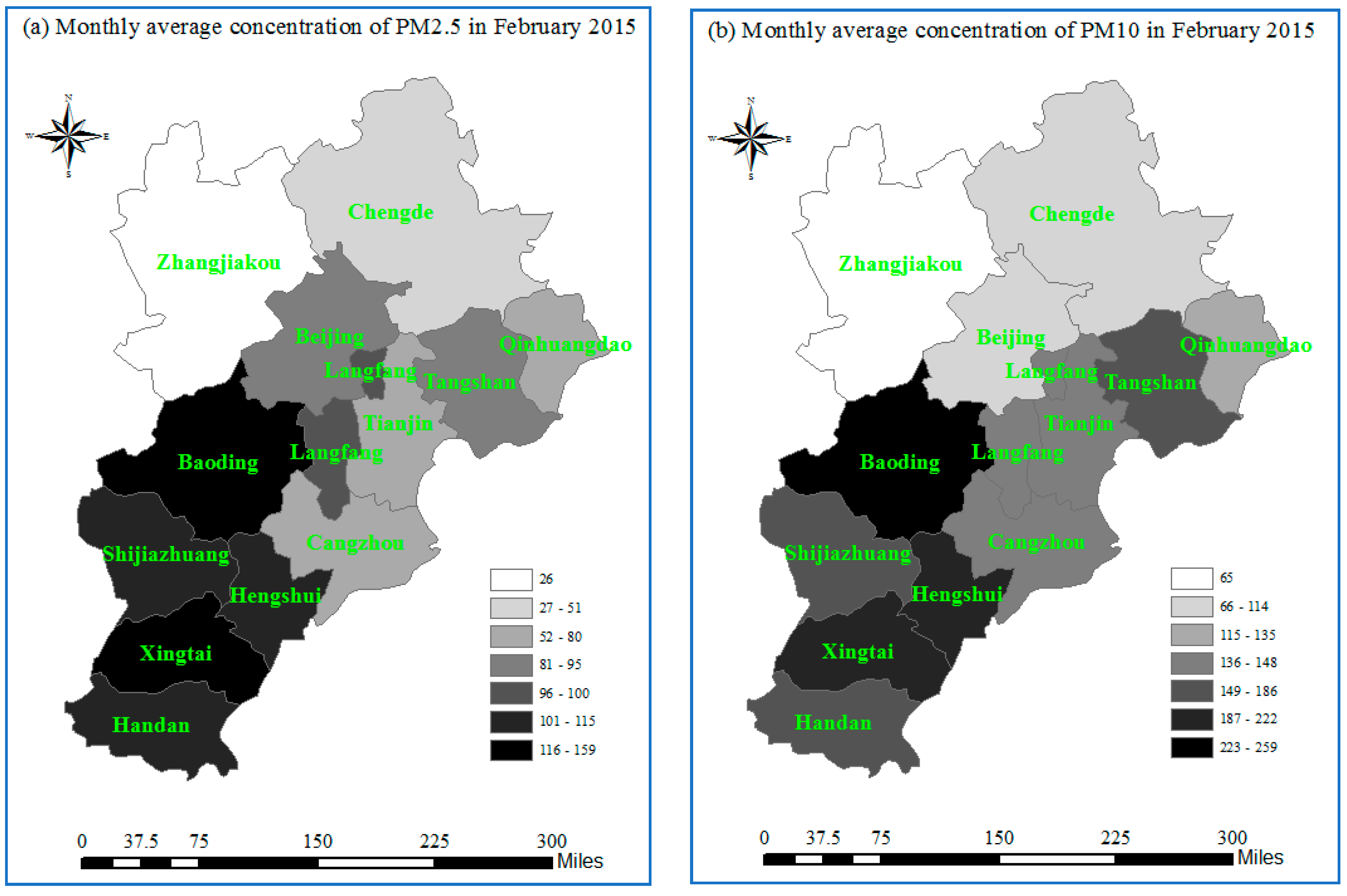
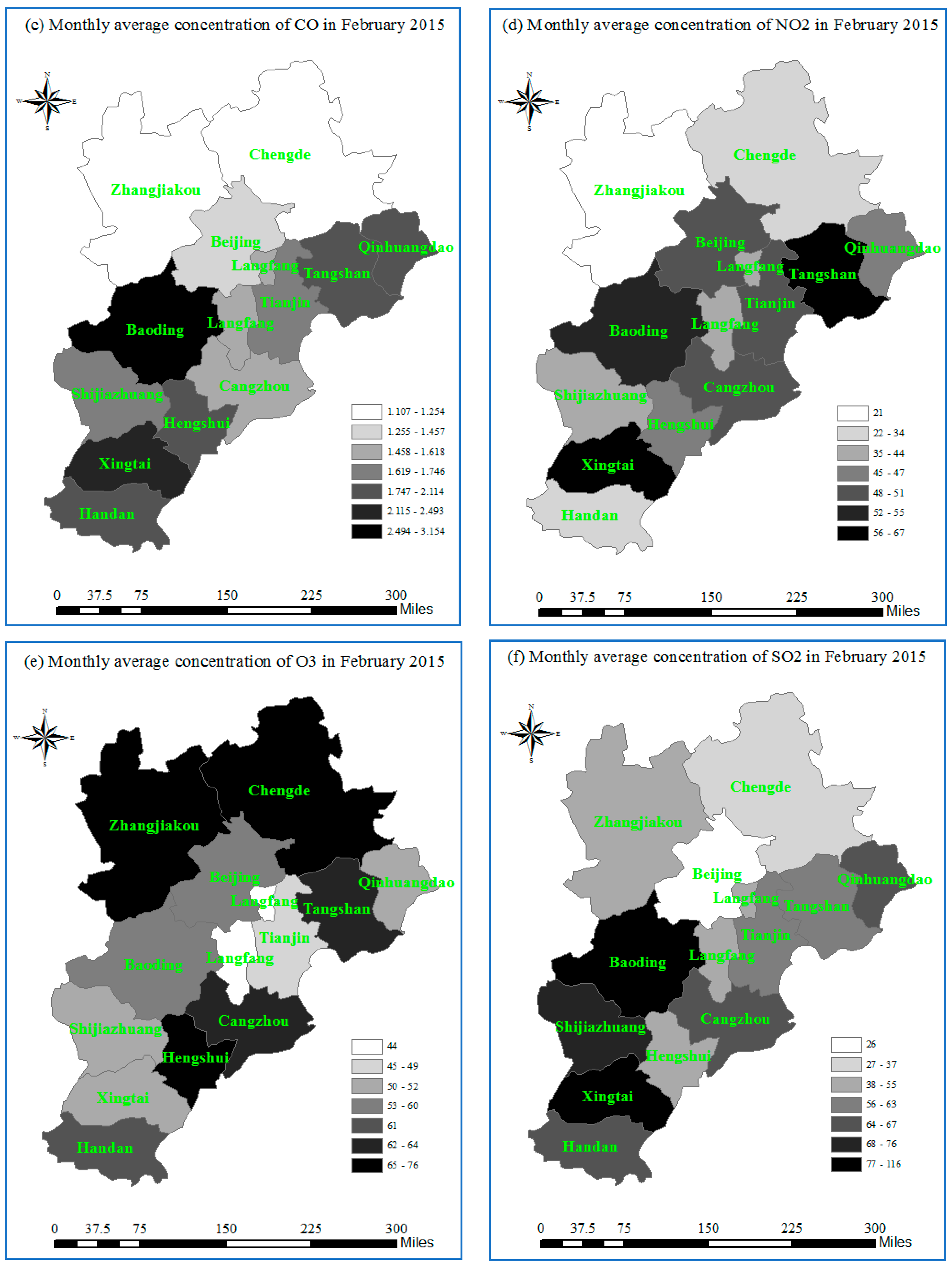
However, none of the above studies considered the combined effects of the six pollutants. In fact, the severity of each pollutant is not all the same in cities in the BTH region (see Figure 1) [23].
Therefore, this paper has extended the indicators defined in “AQI Technical Specifications (Trial Use)” (HJ 633-2012). First, we built an indicator system that covers all six main air pollutants and based on the interval analysis method [24,25], we further constructed three kinds of heterogeneous information (information with different dimensions, such as interval number, mean value, and variance) as well as calculated the standardization form of each pollutant indicator in order to capture the effect of each pollutant on air quality within our study period. Then we adopted the Collaborative Filtering Backward Cloud Model to obtain the different weights for calculation of air quality assessment score of each city based on air pollutant concentration data of the BTH region from February 2015 to January 2018. Furthermore, we simulated the Background Trend Line of the dynamic change in air quality in absence of air pollution control policies in cities of the BTH region with help of the Back Propagation (BP) Neural Network method in order to quantify the influence of government policy on pollution control of different cities. Last but not least, we proposed tailored policy recommendations for air pollution control.
The structure of this paper is as follows: Part 2 introduced the methodology and data used in this paper. Part 3 illustrated our calculation results and analysis of the effect of air pollution control policies on various cities in BTH region since March 2016. Part 4 provided conclusions and related policy recommendations.
2. Materials and Methods
2.1. Data
The data adopted by this paper came from the official daily air quality data and pollutant monitoring data published by the Data Center of China’s Ministry of Environmental Protection [23], the City Air Quality Publishing Platform of China’s National Environmental Monitoring Center [26], as well as local governments of Beijing, Tianjin and Hebei. The data range from February 2015 to January 2018, and included the daily average concentration numbers of 6 main air pollutants (PM2.5, PM10, CO, NO2, O3, and SO2).
2.2. Methods
Because this paper has extended the official AQI indicator system of the Chinese government to six main pollutants and 18 indicators, we first selected 3 variables of heterogeneous information (interval number, mean value, and mean variance) for each indicator, and then obtained the standardization form of these variables by common practice and calculated the distance between heterogeneous information and its positive thresholds (the corresponding minimum value of each attribute indicator during the observation period) and negative thresholds (the corresponding maximum value of each attribute indicator during the observation period). Then we further adopted the Collaborative Filtering Model that helps to sort and select the optimal assessment method given multiple indicators in order to determine the differentiated weights of different indicators. Finally, we calculated the air quality assessment scores of 13 cities by the Backward Cloud Model [27].
2.2.1. Construction and Standardization of Heterogeneous Information
We selected 3 variables of heterogeneous information for each main pollutant indicator—interval number, mean value, and mean variance. Among these variables, the mean value and mean variance can be written as real number . We first obtained the standardization form of as :
in which .
The standardization form of the interval number can be written as:
in which .
2.2.2. Calculate the Distance between the Heterogeneous Information and Its Positive and Negative Thresholds
In order to compare different assessment methods, let and be the positive and negative thresholds of the heterogeneous information respectively, i.e., the extremal solutions of the best case and worst case scenario. Therefore, if represents the attribute value of the indicator, its distance from its positive threshold value, can be calculated by:
While its distance from its negative threshold value, can be calculated by:
2.2.3. Decide Indicator Weights by Using Collaborative Filtering Algorithm
After obtaining the distance between the heterogeneous information from its positive and negative threshold values, we measured the differentiation between various indicators by taking the opposite number of their similarity value calculated by the MSD Similarity Formula.
in which is the differentiation between indicator and ; is the set of all assessment models that cover both and ; is the standardized assessment score of indicator by assessment model .
The mean differentiation of indicator with all other indicators, can be written as:
In equation (8), is the differentiation between the indicator and the indicator . The differential weight of indicator , can be expressed as:
2.2.4. The Backward Cloud Model
In order to combine quantitative and qualitative assessment, we selected Backward Cloud Model with no specific degrees to calculate the air quality score of different cities. First, we obtained the mean value of the air quality scores () based on the information of n indicators ().
This average value is the expected value of air quality of this city. This is the best indicator for qualitative assessment of a city’s air quality.
Given the expected value, we can further calculate the entropy of air quality of different cities, :
This entropy ( means the width of the information, which represents the uncertainty and ambiguity in one city’s air quality score. The bigger the entropy’s value is, the higher the uncertainty becomes.
We then further obtained the hyper entropy of each city’s air quality score through:
in which is the variance of various assessment models against their respective expectation value .
This hyper entropy reflects the uncertainty of various entropy values by showing the dispersion degree of fuzzy information. The bigger the hyper entropy value is, the more disperse a city’s air quality score is, and the more randomness there is. A smaller hyper entropy value means less uncertainty and randomness, and better air quality of a city. The larger the evaluation value obtained, the worse was the air quality of the city at that time. Therefore, with help of the Backward Cloud Model, we obtained the qualitative result expressed by a certain number and realized the integration of quantitative scores and qualitative expression, able to qualitatively describe a city’s air quality based on a quantitative number.
3. Results
With help of the Collaborative Filtering Backward Cloud Model discussed in 3.1 and the MATLAB algorithm we developed (refer to Appendix A) and based on the pollutant data listed in 3.2, we calculated the Air Quality Assessment Score of 13 cities in BTH region from February 2015 to January 2018 (1095 days) as shown below through Table 1, Table 2, Table 3 and Table 4.
Within our study period, the most important air pollution control policy by the Chinese government is the one announced by Prime Minister Li Keqiang in the “Government Work Report” (March 2016) that “we must prioritize the control of air pollution and water pollution with the goal of reducing chemical oxygen demand (COD) and ammonia-nitrogen emissions by 2%, reducing the emissions of sulfur dioxide and oxynitride by 3% and controlling the concentration of PM2.5 in key areas” [28]. As the key area listed in the “Government Work Report”, the BTH region has made great effort on air pollution control under the policy guidance of the central government since March 2016. In order to depict the effect of such air pollution control policy, we adopted the Back Propagation (BP) Neural Network method to simulate the Background Trend Line of the dynamic change in air quality in absence of these pollution control policies in cities of the BTH region, and compared with the actual numbers (especially since the air pollution control campaign that started in March 2016) from below Table 2, Table 3, Table 4 and Table 5, in order to quantify the influence of policy on pollution control of different cities.
By calculations under the Back Propagation (BP) Neural Network (refer to Appendix B for calculation principles and MATLAB algorithm), we obtained the Output Layer result of the Background Trend Line of the dynamic change in air quality in absence of pollution control policies in cities of the BTH region (see Table 5 and Table 6).
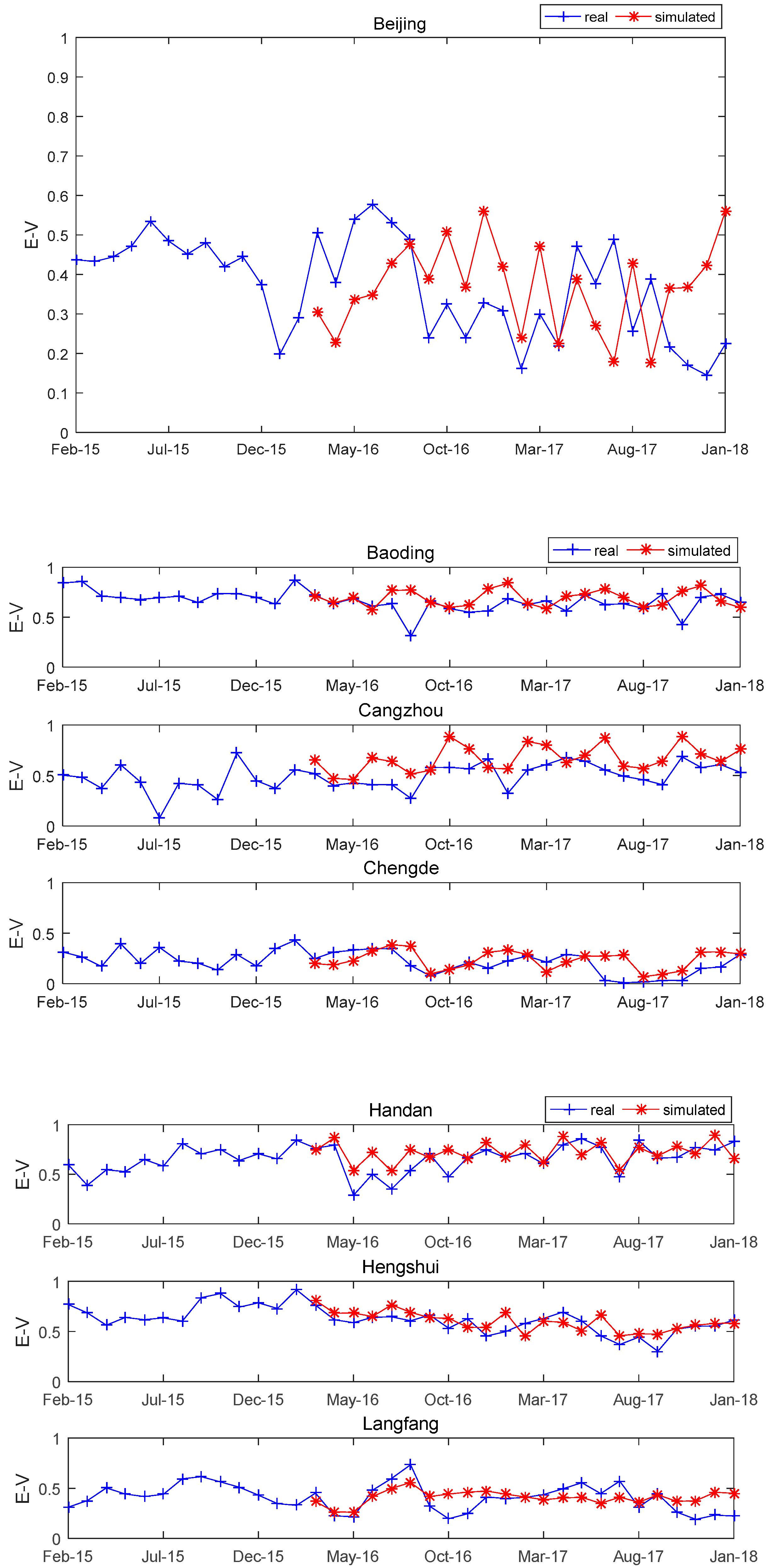
Finally, we can make the comparison between air quality assessment scores simulated by BP Neural Network and actual air quality scores of cities in the BTH region (see Figure 2).
4. Discussion
According to our research method, the larger the evaluation value obtained, the worse was the air quality of the city at that time. Through comparison between the air quality assessment scores simulated by BP Neural Network and the actual air quality scores, we found that the air pollution control policy since March 2016 has shown different effectiveness and impact on cities of the BTH region as below:
(1) Beijing’s air quality scores have shown improvement since August 2016 after the pollution control policy was implemented, but have also experienced fluctuations before April 2017. Beijing has shown success in air pollution control since October 2017, and greatly improved its ranking in air quality among the 13 cities of BTH region from 2017 to 2018. It has even ranked top one for 3 months and ranked among the top three for 8 months in 2017. The air quality of Beijing has improved 55.74% from 0.5057 in March 2016 to 0.2238 in January 2018, and improved 48.82% since the beginning of our study period (February 2015). Behind this remarkable improvement, Beijing has made heavy investment and issued numerous administrative orders with Chinese characteristics.
- From 2016 to 2017, Beijing has invested as much as 34.78 billion RMB in air pollution control, which is almost 7 times of its investment in 2013 [29]. The biggest investment is on “Replacing Coal and Reducing Nitrogen Emission”, i.e., facilitating the energy source change from coal to clean energy and reducing the annual coal consumption of Beijing from 22.7 million tons in 2013 to less than 6 million tons by end of 2017 through administrative orders and equipment upgrade [30]. One of the administrative orders with Chinese characteristics is from Beijing Construction Committee on September 15th 2017 that all road construction work (including any earthwork and house demolition) and hydraulic engineering projects must suspend from November 15th 2017 to March 15th 2018 (the heating season in Beijing) in order to completely eliminate construction dust [31]. Only one month after this administrative order (from October 2017 to January 2018), Beijing has achieved the best air quality score during the entire study period.
- Beijing has prioritized the policy control on high-emission vehicles by extending its forbidden area. In November 2016, Beijing government has issued its revised “Air Pollution Emergency Plan” which stipulates that on days of Air Pollution Orange Alert and Red Alert, all light-duty gasoline vehicles with National Level I and Level II Emission Standards are forbidden on the road in the whole city [32]. Since February 15th 2017, Beijing government has further forbidden cars with National Level I and Level II Emission Standards driving in areas within the 5th Ring Road during workdays (whole day) [33]. By end of 2017, Beijing government has forced the retirement of 2.17 million old motor vehicles, which accounted for 36.12% of its total motor vehicles [30].
- Beijing has implemented more strict elimination policies for polluting companies. The “Production Technology and Equipment Upgrade / Retirement List of Heavy Polluting Industries of Beijing” was officially effective in July 2017, which strictly requires to remove 115 production technologies and 57 production equipment of 11 industries including the steel industry, non-ferrous metals industry, building materials industry, chemical industry, textile printing and dyeing industry, papermaking industry, etc. within a specified time limit and forbids starting or extending any similar projects [34]. By the end of 2017, Beijing government has cleaned up around 11 thousand heavy pollution companies [30]. However, it’s worth noticing that a large number of those companies (especially large industrial companies) simply moved from Beijing to a nearby city. The result is moving the pollution sources from Beijing to Hebei province.
(2) As the other municipality directly under the central government in this region, Tianjin has experienced large fluctuations during the study period. Although its air quality has improved by 34.38% after implementation of the pollution control policies, its air quality score has once dropped to the worst level of 0.7321 in April 2017 and gradually improved afterwards. Its air quality score in January 2018 only improved by 2.04% compared to its level in February 2015. According to the inspection result on Tianjin provided by the Environmental Protection Inspectorate sent by the central government in July 2017, the execution as well as effectiveness of Tianjin’s air pollution control policy has large fluctuations with even worse air quality in several periods. With high concentration of heavy and chemical industries in the city and severe structural pollution, Tianjin still initialized or planned to initialize several thermal power projects without regard to the environment, which resulted in a large increase in the concentration of nitrogen dioxide in the atmosphere in 2016, and an increase of PM2.5 by 27.5% in the first quarter of 2017 [35]. Although thee Tianjin government has taken a series of remedial measures including longer suspension period than Beijing—from October 2017 to March 2018, all road construction work, hydraulic engineering projects, earthwork, house demolition and cement mixing work are paused in Tianjin’s urban area [36]. However, the policy has not shown much effectiveness so far.
(3) Baoding and Cangzhou have shown most overall policy effectiveness within the study period with their own characteristics. Although Baoding has achieved an improvement of 23.41% in air quality score in January 2018 compared with that of the beginning period, except for August 2016 and October 2017, its air quality score has been above 0.50 for most of the study period. Cangzhou has shown lower air quality score than other cities in the study period partly due to its geographical location close to the Bohai Sea. However, since October 2017, its air quality score has deteriorated to above 0.5, resulting in an air quality score in January 2018 that has declined by 6.02% compared with that of the beginning period. We have noticed that in June 2017, Cangzhou Bohai New Area planned a “Beijing Enterprise Zone” in order to receive the immigrating companies of non-capital functions from Beijing. By the end of 2017, almost one thousand companies have settled down in this “Beijing Enterprise Zone”, among which there are nearly 800 clothes manufacturing companies [37].
(4) The air pollution control policy of Handan, Hengshui, Xingtai and Zhangjiakou has shown low effectiveness within the study period with large differences in air quality scores. All these cities have experienced a decline of air quality scores when comparing the last period with the beginning period, except for Hengshui (the score of Handan has declined by 38.68%, that of Zhangjiakou declined by 17.84%, while that of Xingtai declined by 6.98%). We have noticed that these 4 cities have all received large numbers of polluting companies that migrated out of Beijing in the study period. In 2014, Beijing government decided to move its Lingyun Building Materials & Chemical Co.,Ltd. from Beijing to Handan, which was the first central-government-owned enterprise that was forced to migrate out of Beijing during our study period and received its production permit from Handan government in October 2015. Before that, this company emitted 400 thousand tons of carbon dioxide, 9 thousand tons of sulfur dioxide, and 10 thousand tons of dust and fume in Beijing every year [38]. In addition, as one of the leading textile printing and dyeing companies of Beijing, Victor’s Clothing Company also migrated to Hengshui in 2015, only leaving its head office and design center in Beijing [39]. All these migrating companies plus the existing polluting companies in these cities such as Handan Iron and Steel Group Company, panel and plate processing companies in Xingtai, chemical plants in Hengshui, and emissions from the growing numbers of motor vehicles in Zhangjiakou in recent years—the various factors have offset the effects of the air pollution control policies.
(5) The air quality score of Langfang, which is located between the two municipalities directly under the central government—Beijing and Tianjin, dropped to the worst level of 0.7345 in August 2016, ranking bottom among the 13 cities in our study scope. However, after that, its air quality score has seen distinct improvement and reached its best level of 0.2227 in January 2018 (improved by 28.55% compared with its beginning level), ranking top among the 13 cities. Located in the ecological conservation area north-west of Beijing, Chengde has kept an outstanding air quality record of under 0.40. We noticed that the air quality score of Chengde first dropped to the worst level during June and October 2017 but then climbed up. Its air quality score has only improved by 7.37% when comparing that of the ending period with the beginning period. This result shows big fluctuations in air quality and policy effectiveness of these 2 cities in our study period and needs further enhancement in the future.
(6) Tangshan’s case is a little special. Although its air quality in January 2018 has improved by 22.37% compared with the beginning of the period, its air quality score has ranked bottom in 9 months across the study period of 36 months, and has showed no sign of improvement until October 2017. In order to understand the reason behind, we must be aware that from 2014 to 2017, Tangshan received the most industries that migrated from Beijing and Tianjin among cities in Hebei province, with total investment of 575.1 billion RMB and 442 projects of investment over 100 million RMB, including large heavy-pollution industrial companies such as Capital Iron and Steel Company and Beijing Coking and Chemical Plant [40]. The Caofeidian District of Tangshan with large numbers of immigrating companies from Beijing and Tianjin is only one-hour drive from downtown Tangshan [41]. Therefore, the moving-in of industrial companies has caused huge impact on the air quality of Tangshan. That is why Tangshan government appropriated 66.70 million RMB from its fiscal income and constructed an air quality grid monitoring and decision-making support system with high accuracy for the purpose of air pollution monitoring and control which was officially launched in September 2017. This system has integrated resources from various government departments including the environmental protection department, public security department, housing development department and land department, and installed almost 600 miniaturized and integrated online monitoring devices with international standards in the urban area [42]. Moreover, Tangshan has put great emphasis on staggering peak production of iron and steel companies. Since November 15th 2017, Tangshan government has demanded that all of its 35 iron and steel companies adopt staggering-peak production [43]. For example, Tangshan Iron and Steel Co., Ltd. under Hebei Iron and Steel Group has limited its steel production to 477.5 thousand tons of by suspending the operation of blast furnaces [44], which has greatly helped the improvement of air quality since October 2017.
(7) The air pollution control policy has achieved little effect in Shijiazhuang and Qinhuangdao. The air quality score of Shijiazhuang in January 2018 has deteriorated by 58.60% when compared with that of the beginning period. The possible reasons are: First, the geographic location of Shijiazhuang is very close to the Taihang Mountains, which blocks the wind or air circulation and causes air pollutants to linger above the city, creating difficulty for the clean-up of air pollution [45]. Moreover, apart from its own polluting industries including the iron and steel industry and cement industry, Shijiazhuang has also received large numbers of polluting industries from Beijing and Tianjin in recent years, including the building materials industry, leather manufacturing industry, pharmaceuticals industry, etc. [46]. Many of these polluting companies have set their new location to be between Tangshan and Qinhuangdao, which has impacted the air quality of Qinhuangdao and offset the effectiveness of air pollution control policies to some extent [47].
5. Conclusions
This paper calculated and assessed the air quality of 13 cities of the BTH region from February 2015 to January 2018 based on the extended AQI indicator system. By constructing and standardizing Heterogeneous Information of major pollutant indicators including interval number, mean value, and variance, we depicted the important effect of other relevant features of pollutant indicators beyond single-point data. Based on that, we further calculated the air quality scores of different cities in the BTH region by using the Collaborative Filtering Backward Cloud Model to construct differentiated weights of different indicators. With help of the Back Propagation (BP) Neutral Network, we simulated the effect of the pollution control policies of the Chinese government targeting air pollution since March 2016. Our conclusion is: the pollution control policies have improved the air quality of Beijing by 55.74%, and improved the air quality of Tianjin by 34.38%; while the migration of polluting enterprises from Beijing and Tianjin has caused different changes in air quality in different cities of Hebei province—we saw air quality deterioration by 58.60% and 38.68% in Shijiazhuang and Handan city respectively. Based on findings above, we provided below policy recommendations for air pollution control of the BTH region:
(1) Embrace more market measures than administrative orders in the battle against air pollution. Currently, most of the measures targeting the air pollution in BTH region are administrative orders and penalty. Although these administrative orders and penalty have achieved certain results, these tools are not efficient or sustainable enough and do not match with the requirement under market economy. Therefore, in the future battle against air pollution, apart from improving the accuracy of air quality measurement, we should also design more tax categories for specific pollutant emissions, such as carbon tax, sulfur dioxide tax, and PM2.5 tax. At the same time, we should convert the current environmental protection fee to corresponding local tax; decrease the production of pollution products by income effect and substitution effect of tax; encourage companies to save energy [48,49] and cut emissions in order to solve the issue of pollution [50,51].
(2) Improve the compensation system for both economic and environmental loss during industry migration in the BTH region. During the air pollution control campaign of Beijing and Tianjin, large numbers of polluting companies moved to cities in Hebei province, including some heavy pollution companies such as the Capital Iron and Steel Company and Beijing Coking and Chemical Plant that moved to Tangshan, the Lingyun Building Materials & Chemical Co., Ltd. that moved to Handan, Beijing’s No. 1 Machine Tool Plant that moved to Baoding, etc. This impacted the air pollution control work of cities in Hebei province to some extent. Therefore, the BTH region should establish and improve the compensation system for industry migration and industry upgrade in this region. Based on the overall industry plan of this region, the government should be fully aware of the economic development and environmental protection pressure on these destination cities of polluting industries, and offer sufficient compensation in terms of economic development and environmental protection resources in order to realize a fair competition within this region and achieve synergy in regional economic development.
(3) Develop pollution control technologies and continuously improve air quality through technological advancement. On one hand, we should encourage colleges and scientific research institutions in this region to continue working on air pollution control technologies, and enhance the cleansing and control of industrial wastegas and motor vehicle exhaust. On the other hand, we should continuously develop and implement new energy technologies in this region; improve traffic management and green construction in the city; and further reduce pollution by encourage public transportation and other environmentally friendly methods such as walking and cycling.
Author Contributions
G.Y. and W.Y. are joint first authors. They contributed equally to this paper. Conceptualization, W.Y.; Methodology, G.Y. and W.Y.; Resources, G.Y. and W.Y.; Software, G.Y.; Validation, W.Y.; Formal Analysis, G.Y. and W.Y.; Data Curation, G.Y. and W.Y.; Writing—Original Draft Preparation, G.Y. and W.Y.; Writing—Review and Editing, G.Y. and W.Y.
Funding
Guanghui Yuan is financially supported by the National Natural Science Foundation of China (grant number 71271126) and the Graduate Innovation Fund of Shanghai University of Finance and Economics. Weixin Yang is financially supported by the Humanities and Social Sciences Research Fund of the University of Shanghai for Science and Technology, and the Decision-making Consultation Research Project of Shanghai Municipal Government. The authors gratefully acknowledge the above financial supports.
Conflicts of Interest
The authors declare no conflict of interest.
Appendix A. MATLAB algorithm for the Collaborative Filtering Backward Cloud Model
        load(‘DATA.mat’);
        data=DATA;
        L=5;
        a1=max(data(:,1));
        data(:,1)=1-data(:,1)/a1;
        data(:,2)=data(:,2);
        a2=max(max(data(:,4:5)));
        data(:,4:5)=data(:,4:5)/a2;
        a3=max(max(data(:,6:8)));
        data(:,6:8)=data(:,6:8)/a3;
        data1=xiangduizhengtiejindu(data,L);
        MSD=chayi(data1); MSD_=mean(MSD,2);
        MSDsum=sum(MSD_);
        W=MSD_./MSDsum;
        W=W’;
         [Ex,En,He]=nixiangyun(data1,W);

        function [MSD]=chayi(data)
        [m,n]=size(data);
        for i=1:n
        for j=i:n
                AA=[data(:,i) data(:,j)];
                [z1,z2]=find(isnan(AA));
                AA(z1,:)=[[];
                [p,q]=size(AA);
                a=intersect(AA(1),AA(2));
                b=length(a);
                card(i,j)=1-b/(2*p-b);
                %card(i,j)=pdist(AA’, ‘jaccard’);
                qiuhe(i,j)=mean((AA(:,1)-AA(:,2)).^2);
                %qiuhe(i,j)=sum((AA(:,1)-AA(:,2)).^2);
                msd(i,j)=qiuhe(i,j)./card(i,j);
            end
        end
        MSD=msd+msd’;
        for i=1:n
            MSD(i,i)=0;
        end

        function dataZZ=xiangduizhengtiejindu(data,L)
        dataz=max(data);
        dataz(10)=max(data(:,10));
        dataf=min(data);
        dataf(10)=min(data(:,10));
        dataZ(:,1)=(data(:,1)-dataz(1)).^2;
        dataZ(:,2)=1/L.*((data(:,2)+data(:,3)-(dataz(2)+dataz(3))).^2);
        dataZ(:,3)=1/2.*(((data(:,4)-dataz(4)).^2+(data(:,5)-dataz(5)).^2));
        dataZ(:,4)=1/3.*((data(:,6)-dataz(6)).^2+(data(:,7)-dataz(7)).^2+(data(:,8)-dataz(8)).^2);
        dataZ(:,5)=1/3.*((data(:,9)-dataz(9)).^2+(data(:,10)-dataz(10)).^2+((data(:,9)+data(:,10))-(dataz(9)+dataz(10))).^2);
        dataF(:,1)=(data(:,1)-dataf(1)).^2;
        dataF(:,2)=1/L.*((data(:,2)+data(:,3)-(dataf(2)+dataf(3))).^2);
        dataF(:,3)=1/2.*(((data(:,4)-dataf(4)).^2+(data(:,5)-dataf(5)).^2));
        dataF(:,4)=1/3.*((data(:,6)-dataf(6)).^2+(data(:,7)-dataf(7)).^2+(data(:,8)-dataf(8)).^2);
        dataF(:,5)=1/3.*((data(:,9)-dataf(9)).^2+(data(:,10)-dataf(10)).^2+((data(:,9)+data(:,10))-(dataf(9)+dataf(10))).^2);
        dataZZ=dataZ./(dataZ+dataF);

        function [Ex,En,He]=nixiangyun(UU,W)
        UU=mapminmax(UU’,0,1);
        UU=UU’;
        [m,n]=size(UU);
        X_=W*UU’;
        Ex=X_;
        sum1=zeros(1,m);
        En=zeros(1,m);
        for i=1:m
        for j=1:n
                   BB=abs(UU(i,j)-X_(i));
                   sum1(i)=sum1(i)+BB;
            end
            En(i)=(pi/2)^2*mean(sum1(i),2);
        end
        S2=zeros(1,m);
        for i=1:m
            S2(i)=var(UU(i,:));
        end
        He=zeros(1,m);
        for i=1:m
            He(i)=(abs(S2(i)-En(i)^2))^0.5;
        end
Appendix B: Calculation Principles of BP Neural Network and MATLAB algorithm
Appendix B.1. Calculation Principles of BP Neural Network
In March 2016, Chinese Prime Minister Li Keqiang officially raised in the “Government Work Report” that we must prioritize the control of air pollution and water pollution with the goal of reducing chemical oxygen demand (COD) and ammonia-nitrogen emissions by 2%, reducing the emissions of sulfur dioxide and oxynitride by 3% and controlling the concentration of PM2.5 in key areas including Beijing, Tianjin and Hebei [28]. Since March 2016, the Chinese government has made great effort in air pollution control under the aligned policy guidance of the central government. In order to depict the effect of such air pollution control policy, we adopted the Back Propagation (BP) Neural Network method to simulate the Background Trend Line of the dynamic change in air quality in absence of these pollution control policies in cities of the Beijing-Tianjin-Hebei (BTH) region in order to quantify the influence of policy on pollution control of different cities.
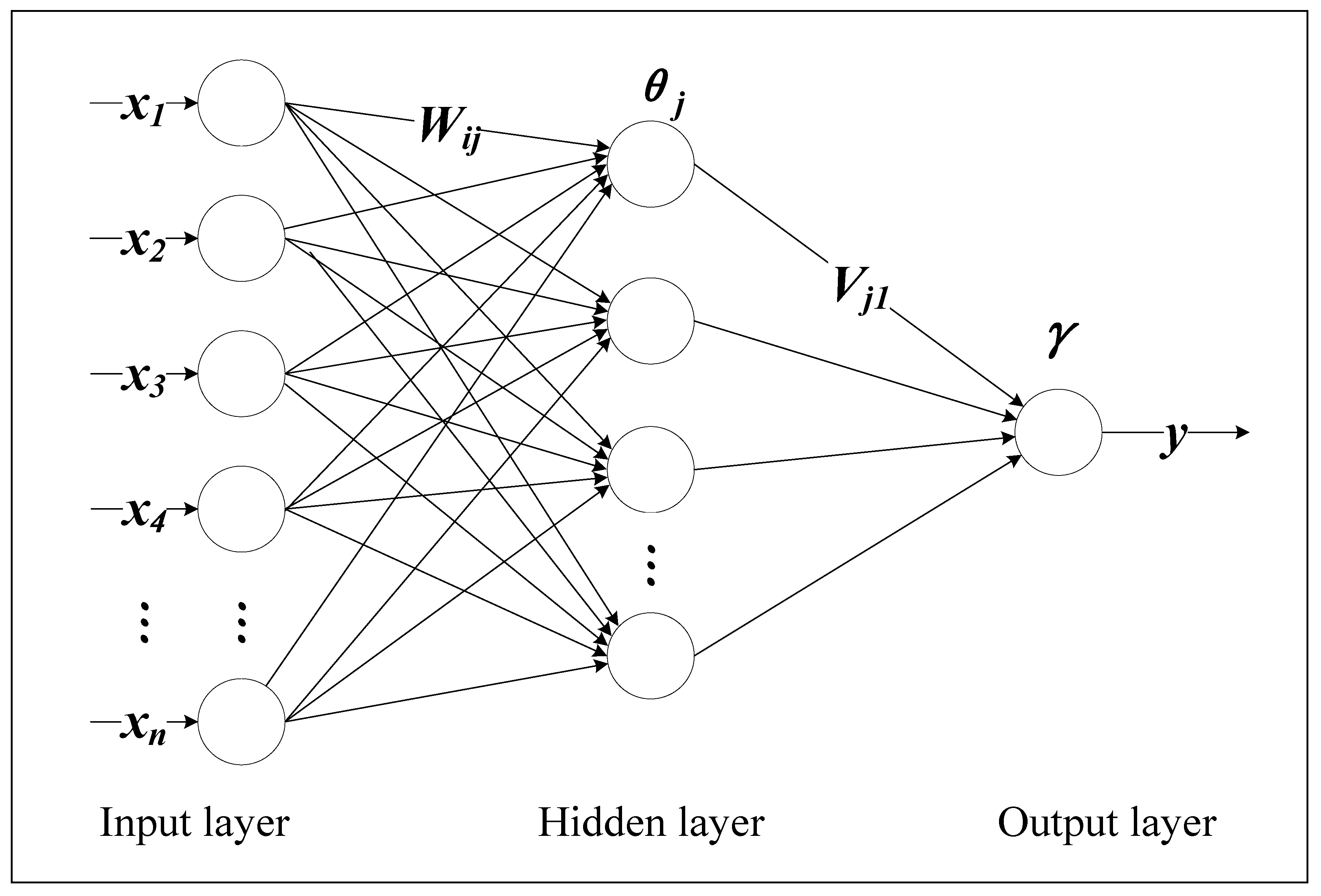
The BP Neural Network is a multilayered feedforward network, consisting of the Input Layer, Hidden Layer and Output Layer. In calculations and predictions related to policy analysis, the BP Neural Network with single hidden layer can approximate any continuous function in a bounded region with any specified precision [52]. In our model, the number of neurons (nodes) on the input and output layers of the BP Neural Network equals the number of dimensions of our input vector (pollutant data) and output vector (assessment score). Its topological structure is shown in Figure A1, in which represents the Input Vector of pollutant data in the past n days while the expectation value of the (n+1)th day is y. Let the number of nodes on the hidden layer be m, the link weight between the input layer and hidden layer be , the link weight between the hidden layer and output layer be , and the thresholds of nodes on the hidden layer and output layer be and respectively.
Figure A1.
Structure of Single Hidden Layer, Single Output BP Neural Network.

Through forward propagating of input signals (pollutant data) and back propagation of error signals, we can complete the calculation process of such BP Neural Network: propagating the pollutant input vector through the Input Layer, Hidden Layer and Output Layer, and obtaining the estimated output of (assessment score) on the Output Layer by using the link weight of , and between different layers as well as randomly assigned threshold values of and and the activation function; propagating —the error between the output value and the expected value of through the Input Layer, Hidden Layer and Output Layer, and modifying the link weights between different layers towards the direction of diminishing errors. Assume the number of learning samples is p, expressed by a vector of . After obtaining the output vector of the pth sample, we could calculate the error of the pth sample by the square error function.
In above equation, is the expected output.
The global error with p samples is:
(1) Output Layer Weight Change
Using the BP algorithm of accumulative error to modify in order to minimize the global error of E:
The error signal in above equation is:
(2) Hidden Layer Weight Change
The equation for weight adjustment of neural networks on the Hidden Layer is as follows:
Appendix B.2. MATLAB Algorithm
          function [A]=BP(BB)
           [N,M]=size(BB);
          for kk=1:N
              x=BB(kk,:);
          lag=6;
          iinput=x;
          n=length(iinput);
          inputs=zeros(lag,n-lag);
          for i=1:n-lag
              inputs(:,i)=iinput(i:i+lag-1)’;
          end
          targets=x(lag+1:end);
          hiddenLayerSize = 10;
          net = fitnet(hiddenLayerSize);
          net.divideParam.trainRatio = 70/100;
          net.divideParam.valRatio = 15/100;
          net.divideParam.testRatio = 15/100;
           [net,tr] = train(net,inputs,targets);
          yn=net(inputs);
          errors=targets-yn;
          errorsA(kk,:)=errors;

          fn=23;

          f_in=iinput(n-lag+1:end)’;
          f_out=zeros(1,fn);
          for i=1:fn
              f_out(i)=net(f_in);
              f_in=[f_in(2:end);f_out(i)];
          end
          A(kk,:)=f_out;
          end
          end
References
- Australia State of the Environment National Air Quality Standards: Ambient Air Quality. 2016. Available online: https://soe.environment.gov.au/theme/ambient-air-quality/topic/2016/national-air-quality-standards (accessed on 18 December 2018).
- Yang, W.; Li, L. Efficiency evaluation of industrial waste gas control in China: A study based on data envelopment analysis (DEA) model. J. Clean. Prod. 2018, 179, 1–11. [Google Scholar] [CrossRef]
- Su, P.; Lin, D.; Qian, C. Study on Air Pollution and Control Investment from the Perspective of the Environmental Theory Model: A Case Study in China, 2005–2014. Sustainability 2018, 10, 2181. [Google Scholar] [CrossRef]
- Yang, Y.; Yang, W. Does Whistleblowing Work for Air Pollution Control in China? A Study Based on Three-party Evolutionary Game Model under Incomplete Information. Sustainability 2019, 11, 324. [Google Scholar] [CrossRef]
- Ministry of Environmental Protection of the People’s Republic of China. Technical Regulation on Ambient Air Quality Index (on Trial): HJ 633-2012; China Environmental Science Press: Beijing, China, 2012.
- ISO 4220. Ambient Air—Determination of a Gaseous Acid Air Pollution Index—Titrimetric method with Indicator or Potentiometric End-Point Detection; International Organization for Standardization: Geneva, Switzerland, 1983. [Google Scholar]
- Ministry of Environmental Protection of the People’s Republic of China. Ambient Air Quality Standards: GB3095-2012; China Environmental Science Press: Beijing, China, 2012.
- Xinhuanet. Hebei’s air quality “burst” and PM2.5 Index in Shijiazhuang is over 1000. Available online: http://www.xinhuanet.com/local/2016-12/19/c_129411383.htm (accessed on 21 April 2018).
- People’s Central Broadcasting Station What is the Feeling When the PM2.5 Index has Exceeded 1400? Look at Shenyang. Available online: http://news.cnr.cn/native/gd/20151109/t20151109_520447867.shtml (accessed on 21 April 2018).
- Ministry of Environmental Protection of the People’s Republic of China. The “Twelfth Five-Year Plan” for Prevention and Control of Atmospheric Pollution in Key Regions; Clean Air Alliance of China: Beijing, China, 2012.
- Lang, J.; Cheng, S.; Wei, W.; Zhou, Y.; Wei, X.; Chen, D. A study on the trends of vehicular emissions in the Beijing-Tianjin-Hebei (BTH) region, China. Atmos. Environ. 2012, 62, 605–614. [Google Scholar] [CrossRef]
- Xu, J.; Wang, X.; Zhang, S. Risk-based air pollutants management at regional levels. Environ. Sci. Policy 2013, 25, 167–175. [Google Scholar] [CrossRef]
- Zhao, P.; Dong, F.; Yang, Y.; He, D.; Zhao, X.; Zhang, W.; Yao, Q.; Liu, H. Characteristics of carbonaceous aerosol in the region of Beijing, Tianjin, and Hebei, China. Atmos. Environ. 2013, 71, 389–398. [Google Scholar] [CrossRef]
- Sheng, L.; Lu, K.; Ma, X.; Hu, J.; Song, Z.; Huang, S.; Zhang, J. The air quality of Beijing-Tianjin-Hebei regions around the Asia-Pacific Economic Cooperation (APEC) meetings. Atmos. Pollut. Res. 2015, 6, 1066–1072. [Google Scholar] [CrossRef]
- Miao, Y.; Liu, S.; Zheng, Y.; Wang, S.; Chen, B.; Zheng, H.; Zhao, J. Numerical study of the effects of local atmospheric circulations on a pollution event over Beijing-Tianjin-Hebei, China. J. Environ. Sci. 2015, 30, 9–20. [Google Scholar] [CrossRef]
- Zhou, Y.; Cheng, S.; Lang, J.; Chen, D.; Zhao, B.; Liu, C.; Xu, R.; Li, T. A comprehensive ammonia emission inventory with high-resolution and its evaluation in the Beijing-Tianjin-Hebei (BTH) region, China. Atmos. Environ. 2015, 106, 305–317. [Google Scholar] [CrossRef]
- Han, F.; Xu, J.; He, Y.; Dang, H.; Yang, X.; Meng, F. Vertical structure of foggy haze over the Beijing-Tianjin-Hebei area in January 2013. Atmos. Environ. 2016, 139, 192–204. [Google Scholar] [CrossRef]
- Guo, X.; Fu, L.; Ji, M.; Lang, J.; Chen, D.; Cheng, S. Scenario analysis to vehicular emission reduction in Beijing-Tianjin-Hebei (BTH) region, China. Environ. Pollut. 2016, 216, 470–479. [Google Scholar] [CrossRef] [PubMed]
- Chen, L.; Shi, M.; Li, S.; Gao, S.; Zhang, H.; Sun, Y.; Mao, J.; Bai, Z.; Wang, Z.; Zhou, J. Quantifying public health benefits of environmental strategy of PM2.5 air quality management in Beijing-Tianjin-Hebei region, China. J. Environ. Sci. 2017, 57, 33–40. [Google Scholar] [CrossRef] [PubMed]
- Zhu, L.; Gan, Q.; Liu, Y.; Yan, Z. The impact of foreign direct investment on SO2 emissions in the Beijing-Tianjin-Hebei region: A spatial econometric analysis. J. Clean. Prod. 2017, 166, 189–196. [Google Scholar] [CrossRef]
- Wang, Y.; Liu, H.; Mao, G.; Zuo, J.; Ma, J. Inter-regional and sectoral linkage analysis of air pollution in Beijing-Tianjin-Hebei (Jing-Jin-Ji) urban agglomeration of China. J. Clean. Prod. 2017, 165, 1436–1444. [Google Scholar] [CrossRef]
- Zhang, X.; Shi, M.; Li, Y.; Pang, R.; Xiang, N. Correlating PM2.5 concentrations with air pollutant emissions: A longitudinal study of the Beijing-Tianjin-Hebei region. J. Clean. Prod. 2018, 179, 103–113. [Google Scholar] [CrossRef]
- Data Center of China’s Ministry of Environmental Protection. Concentration of main pollutants in the PRD Region, 2015–2018. Available online: http://datacenter.sepa.gov.cn/ (accessed on 17 July 2018).
- Wang, S.Y.; Zhu, S.S. On fuzzy portfolio selection problems. Fuzzy Optim. Decis. Mak. 2002, 1, 361–377. [Google Scholar] [CrossRef]
- Xu, W.; Ma, J.; Wang, S.Y.; Hao, G. Vague soft sets and their properties. Comput. Math. Appl. 2010, 59, 787–794. [Google Scholar] [CrossRef] [Green Version]
- China’s National Environmental Monitoring Center. The City Air Quality Publishing Platform. Available online: http://106.37.208.233:20035/ (accessed on 17 July 2018).
- Geng, X.; Dong, X. Concept evaluation approach based on rough information axiom and Cloud Model. Comput. Integr. Manuf. Syst. 2017, 23, 661–669. [Google Scholar]
- Li, K. Government Work Report at the Fourth Session of the Twelfth National People’s Congress (March 5, 2016); People’s Publishing House: Beijing, China, 2016. [Google Scholar]
- Luo, Q. Beijing’s investment in atmospheric governance exceeds 30 billion yuan in two years. Beijing Daily. 13 December 2017. Available online: http://bjrb.bjd.com.cn/html/2017-12/13/content_202216.htm (accessed on 12 February 2019).
- Chen, J. Beijing Municipal Government Work Report at the First Session of the Fifteenth Beijing Municipal People’s Congress (January 24, 2018); Beijing Daily: Beijing, China, 2018. [Google Scholar]
- Beijing Municipal Commission of Housing and Urban-Rural Development. Detailed Implementation Plan for Beijing of the “Action Plan for Comprehensive Prevention and Control of Atmospheric Pollution in the Beijing-Tianjin-Hebei Region and the Surrounding Areas in the Autumn and Winter 2017–2018”; Beijing Municipal Commission of Housing and Urban-Rural Development: Beijing, China, 2017.
- Beijing Municipal People’s Government. Beijing Municipal Air Heavy Pollution Emergency Plan (2016 Edition); Beijing Municipal People’s Government: Beijing, China, 2016.
- Yang, X. Cars with National Level I and Level II Emission Standards are forbidden within the 5th Ring Road of Beijing during workdays. Economic Daily, 2017 13 February. [Google Scholar]
- Beijing Municipal People’s Government. Production Technology and Equipment Upgrade & Retirement List of Heavy Polluting Industries of Beijing (2017 Edition); Beijing Municipal People’s Government: Beijing, China, 2017.
- The First Environmental Protection Inspectorate of the Central Government. 2017 Tianjin Environmental Protection Supervision Report; The First Environmental Protection Inspectorate of the Central Government: Tianjin, China, 2017. [Google Scholar]
- Tianjin Municipal People’s Government. The Action Plan for the Comprehensive Prevention and Control of Atmospheric Pollution in the Autumn and Winter of 2017-2018 in Tianjin; Tianjin Municipal People’s Government: Tianjin, China, 2017.
- SOHU Finance Cangzhou Bohai New Area: Beijing’s First Choice for Corporate Relocation. Available online: http://www.sohu.com/a/150424973_232843 (accessed on 21 April 2018).
- China Economic Net Lingyun Building Materials & Chemical Co.,Ltd., Beijing’s first Central-Government-Owned Enterprise Relocated in Handan. Available online: http://www.ce.cn/cysc/yq/dt/201405/16/t20140516_2824568.shtml (accessed on 21 April 2018).
- Hebei Provincial People’s Government. From Contract to Production: The 18 Months of Victor’s Relocation to Hengshui; Hebei Provincial People’s Government: Hengshui, China, 2015.
- Xinhua News Agency Tangshan: Undertaking the Transfer of Beijing and Tianjin Industry and Promoting Economic Development. Available online: http://www.xinhuanet.com/photo/2018-03/24/c_1122585335.htm (accessed on 21 April 2018).
- Wang, Q.; Li, B. Enterprises migrated to Caofeidian from Beijing. People’s Daily. 22 December 2017. Available online: http://paper.people.com.cn/rmrb/html/2017-12/22/nw.D110000renmrb_20171222_3-14.htm (accessed on 12 February 2019).
- Tangshan Environmental Protection Bureau. Public Tender Announcement for Accurate Monitoring and Decision Support System for Grid Pollution Control of Air Pollution in Tangshan; Tangshan Environmental Protection Bureau: Tangshan, China, 2017. [Google Scholar]
- Tangshan Municipal People’s Government. The scheme of Staggering-Peak Production for Tangshan City’s Steel Industry in 2017–2018 Heating Season; Tangshan Municipal People’s Government: Tangshan, China, 2017.
- Hebei Provincial Department of Environmental Protection Beijing Evening News: Fighting for the blue sky in Tangshan. Available online: http://www.hebhb.gov.cn/xwzx/mtbb/201712/t20171214_58883.html (accessed on 21 April 2018).
- Chen, J.; Zhang, Y.; Yang, P.; Qian, W.; Wang, X.; Han, J. Pollution process and optical properties during a dust aerosol event in Shijiazhuang. China Environ. Sci. 2016, 36, 979–989. [Google Scholar]
- Kang, A.; Li, Y.; Zhang, B.; Zhong, H. Reasons and Treatment Measures of Haze Formation in Shijiazhuang City. J. Hebei Univ. Econ. Bus. Compr. Ed. 2015, 15, 89–90, 100. [Google Scholar]
- Zhang, B.; Cao, J.; Du, J.; Sun, L. The Distribution of The Atmospheric Pollutants and Its Weather Background in Qinhuangdao. J. Environ. Manag. Coll. China 2016, 26, 79–82. [Google Scholar]
- Yang, W.; Li, L. Energy Efficiency, Ownership Structure, and Sustainable Development: Evidence from China. Sustainability 2017, 9, 912. [Google Scholar] [CrossRef]
- Yang, W.; Li, L. Analysis of Total Factor Efficiency of Water Resource and Energy in China: A Study Based on DEA-SBM Model. Sustainability 2017, 9, 1316. [Google Scholar] [CrossRef]
- Yang, W.; Li, L. Efficiency Evaluation and Policy Analysis of Industrial Wastewater Control in China. Energies 2017, 10, 1201. [Google Scholar] [CrossRef]
- Li, L.; Yang, W. Total Factor Efficiency Study on China’s Industrial Coal Input and Wastewater Control with Dual Target Variables. Sustainability 2018, 10, 2121. [Google Scholar] [CrossRef]
- Veelenturf, L.P.J. Analysis and Applications of Artificial Neural Networks; Prentice Hall: London, UK, 1995. [Google Scholar]
Figure 1.
Monthly average concentration of six pollutants in the BTH Region (February 2015): (a) PM2.5 (unit: ); (b) PM10 (unit: ); (c) CO (unit: ); (d) NO2 (unit: ); (e) O3 (unit: ); (f) SO2 (unit: ).
Figure 1.
Monthly average concentration of six pollutants in the BTH Region (February 2015): (a) PM2.5 (unit: ); (b) PM10 (unit: ); (c) CO (unit: ); (d) NO2 (unit: ); (e) O3 (unit: ); (f) SO2 (unit: ).


Figure 2.
Comparison between air quality assessment scores simulated by BP Neural Network and actual air quality scores of cities in the BTH region.
Figure 2.
Comparison between air quality assessment scores simulated by BP Neural Network and actual air quality scores of cities in the BTH region.


Table 1.
Air quality assessment score of cities in the BTH region (2015.02–2015.10).
| 2015-02 | 2015-03 | 2015-04 | 2015-05 | 2015-06 | 2015-07 | 2015-08 | 2015-09 | 2015-10 | |
|---|---|---|---|---|---|---|---|---|---|
| Baoding | 0.8440 | 0.8561 | 0.7136 | 0.6942 | 0.6789 | 0.6942 | 0.7094 | 0.6473 | 0.7373 |
| Beijing | 0.4373 | 0.4329 | 0.4446 | 0.4723 | 0.5354 | 0.4845 | 0.4516 | 0.4808 | 0.4200 |
| Cangzhou | 0.5017 | 0.4831 | 0.3742 | 0.6043 | 0.4379 | 0.0800 | 0.4219 | 0.4058 | 0.2640 |
| Chengde | 0.3135 | 0.2663 | 0.1712 | 0.3941 | 0.1988 | 0.3590 | 0.2240 | 0.2055 | 0.1351 |
| Handan | 0.5969 | 0.3893 | 0.5457 | 0.5285 | 0.6499 | 0.5829 | 0.8147 | 0.7053 | 0.7513 |
| Hengshui | 0.7697 | 0.6868 | 0.5638 | 0.6405 | 0.6189 | 0.6357 | 0.6046 | 0.8389 | 0.8801 |
| Langfang | 0.3117 | 0.3767 | 0.5031 | 0.4415 | 0.4170 | 0.4393 | 0.5946 | 0.6149 | 0.5629 |
| Qinhuangdao | 0.3005 | 0.3197 | 0.3800 | 0.3050 | 0.1375 | 0.1286 | 0.2647 | 0.1929 | 0.1937 |
| Shijiazhuang | 0.4626 | 0.6096 | 0.5823 | 0.3846 | 0.4678 | 0.2947 | 0.4143 | 0.4639 | 0.4341 |
| Tangshan | 0.6236 | 0.8502 | 0.9725 | 0.9995 | 0.7670 | 0.7661 | 0.6697 | 0.7291 | 0.7173 |
| Tianjin | 0.3130 | 0.3760 | 0.0886 | 0.2781 | 0.4627 | 0.0627 | 0.2310 | 0.2190 | 0.2366 |
| Xingtai | 0.7590 | 0.6527 | 0.5737 | 0.5618 | 0.7026 | 0.6843 | 0.8039 | 0.7065 | 0.7335 |
| Zhangjiakou | 0.2422 | 0.2290 | 0.2675 | 0.4207 | 0.2968 | 0.1705 | 0.2582 | 0.1371 | 0.0819 |
Table 2.
Air quality assessment score of cities in the BTH region (2015.11–2016.07).
| 2015-11 | 2015-12 | 2016-01 | 2016-02 | 2016-03 | 2016-04 | 2016-05 | 2016-06 | 2016-07 | |
|---|---|---|---|---|---|---|---|---|---|
| Baoding | 0.7371 | 0.6991 | 0.6298 | 0.8750 | 0.7225 | 0.6364 | 0.6870 | 0.6127 | 0.6329 |
| Beijing | 0.4446 | 0.3742 | 0.1996 | 0.2896 | 0.5057 | 0.3786 | 0.5397 | 0.5779 | 0.5328 |
| Cangzhou | 0.7212 | 0.4504 | 0.3726 | 0.5587 | 0.5211 | 0.4021 | 0.4265 | 0.4103 | 0.4098 |
| Chengde | 0.2902 | 0.1759 | 0.3461 | 0.4294 | 0.2476 | 0.3135 | 0.3312 | 0.3481 | 0.3446 |
| Handan | 0.6415 | 0.7078 | 0.6554 | 0.8445 | 0.7648 | 0.7955 | 0.2903 | 0.5024 | 0.3518 |
| Hengshui | 0.7449 | 0.7871 | 0.7306 | 0.9171 | 0.7632 | 0.6172 | 0.5894 | 0.6422 | 0.6467 |
| Langfang | 0.5093 | 0.4317 | 0.3473 | 0.3294 | 0.4516 | 0.2237 | 0.2164 | 0.4799 | 0.5971 |
| Qinhuangdao | 0.2070 | 0.1576 | 0.0904 | 0.1124 | 0.2889 | 0.3187 | 0.3366 | 0.2894 | 0.1180 |
| Shijiazhuang | 0.6835 | 0.5144 | 0.5899 | 0.6014 | 0.7660 | 0.3267 | 0.5278 | 0.4469 | 0.5410 |
| Tangshan | 0.6982 | 0.4357 | 0.4623 | 0.6462 | 0.8139 | 0.7107 | 0.8880 | 0.9609 | 0.5922 |
| Tianjin | 0.4943 | 0.2709 | 0.2772 | 0.1672 | 0.4672 | 0.4470 | 0.3450 | 0.4395 | 0.0983 |
| Xingtai | 0.6978 | 0.6196 | 0.6253 | 0.7029 | 0.7446 | 0.5027 | 0.5205 | 0.5598 | 0.7750 |
| Zhangjiakou | 0.4137 | 0.2942 | 0.3691 | 0.3947 | 0.2122 | 0.1761 | 0.1561 | 0.0899 | 0.2541 |
Table 3.
Air quality assessment score of cities in the BTH region (2016.08–2017.04).
| 2016-08 | 2016-09 | 2016-10 | 2016-11 | 2016-12 | 2017-01 | 2017-02 | 2017-03 | 2017-04 | |
|---|---|---|---|---|---|---|---|---|---|
| Baoding | 0.3092 | 0.6628 | 0.5853 | 0.5509 | 0.5631 | 0.6854 | 0.6255 | 0.6643 | 0.5634 |
| Beijing | 0.4877 | 0.2403 | 0.3245 | 0.2401 | 0.3293 | 0.3087 | 0.1616 | 0.3003 | 0.2197 |
| Cangzhou | 0.2731 | 0.5797 | 0.5798 | 0.5681 | 0.6649 | 0.3238 | 0.5536 | 0.6097 | 0.6751 |
| Chengde | 0.1787 | 0.0767 | 0.1436 | 0.2105 | 0.1548 | 0.2277 | 0.2727 | 0.2135 | 0.2898 |
| Handan | 0.5420 | 0.7057 | 0.4738 | 0.6708 | 0.7452 | 0.6672 | 0.7120 | 0.6064 | 0.7989 |
| Hengshui | 0.6088 | 0.6651 | 0.5344 | 0.6288 | 0.4565 | 0.5000 | 0.5819 | 0.6314 | 0.6944 |
| Langfang | 0.7345 | 0.3213 | 0.1966 | 0.2460 | 0.4123 | 0.3987 | 0.4081 | 0.4372 | 0.4947 |
| Qinhuangdao | 0.2415 | 0.2363 | 0.2490 | 0.2354 | 0.2881 | 0.4494 | 0.3947 | 0.4700 | 0.4536 |
| Shijiazhuang | 0.4370 | 0.6672 | 0.7702 | 0.7248 | 0.6939 | 0.6808 | 0.7176 | 0.7575 | 0.5961 |
| Tangshan | 0.4957 | 0.7255 | 0.6287 | 0.5398 | 0.5315 | 0.4429 | 0.5363 | 0.6436 | 0.7999 |
| Tianjin | 0.2715 | 0.4562 | 0.3333 | 0.3651 | 0.3652 | 0.3113 | 0.3510 | 0.6127 | 0.7321 |
| Xingtai | 0.3989 | 0.7404 | 0.5957 | 0.5495 | 0.6229 | 0.6827 | 0.8329 | 0.7001 | 0.5804 |
| Zhangjiakou | 0.2147 | 0.0795 | 0.2242 | 0.2973 | 0.2653 | 0.3020 | 0.2287 | 0.1595 | 0.3066 |
Table 4.
Air quality assessment score of cities in the BTH region (2017.05-2018.01).
| 2017-05 | 2017-06 | 2017-07 | 2017-08 | 2017-09 | 2017-10 | 2017-11 | 2017-12 | 2018-01 | |
|---|---|---|---|---|---|---|---|---|---|
| Baoding | 0.7170 | 0.6288 | 0.6332 | 0.5885 | 0.7320 | 0.4273 | 0.7028 | 0.7288 | 0.6464 |
| Beijing | 0.4714 | 0.3771 | 0.4886 | 0.2573 | 0.3874 | 0.2164 | 0.1696 | 0.1455 | 0.2238 |
| Cangzhou | 0.6445 | 0.5570 | 0.4912 | 0.4590 | 0.4080 | 0.6839 | 0.5789 | 0.6079 | 0.5319 |
| Chengde | 0.2721 | 0.0333 | 0.0113 | 0.0156 | 0.0321 | 0.0345 | 0.1520 | 0.1651 | 0.2904 |
| Handan | 0.8597 | 0.7773 | 0.4710 | 0.8398 | 0.6658 | 0.6679 | 0.7722 | 0.7462 | 0.8278 |
| Hengshui | 0.6058 | 0.4576 | 0.3713 | 0.4443 | 0.3034 | 0.5248 | 0.5525 | 0.5562 | 0.6148 |
| Langfang | 0.5550 | 0.4469 | 0.5713 | 0.3136 | 0.4420 | 0.2623 | 0.1900 | 0.2319 | 0.2227 |
| Qinhuangdao | 0.1415 | 0.3120 | 0.2403 | 0.2963 | 0.3901 | 0.4707 | 0.4547 | 0.3096 | 0.2895 |
| Shijiazhuang | 0.8026 | 0.7218 | 0.7478 | 0.6380 | 0.7405 | 0.5206 | 0.6798 | 0.6535 | 0.7337 |
| Tangshan | 0.8857 | 0.8552 | 0.7815 | 0.7767 | 0.7740 | 0.9348 | 0.6063 | 0.5592 | 0.4841 |
| Tianjin | 0.5620 | 0.2684 | 0.3644 | 0.3660 | 0.4094 | 0.4932 | 0.3299 | 0.3422 | 0.3066 |
| Xingtai | 0.9449 | 0.8580 | 0.8058 | 0.8240 | 0.7968 | 0.7023 | 0.8016 | 0.7332 | 0.8120 |
| Zhangjiakou | 0.2200 | 0.1316 | 0.3945 | 0.1164 | 0.0076 | 0.1465 | 0.2841 | 0.3168 | 0.2854 |
Table 5.
Air quality assessment score of cities in the BTH region in absence of pollution control policies simulated by BP Neural Network (2016.03–2017.02).
Table 5.
Air quality assessment score of cities in the BTH region in absence of pollution control policies simulated by BP Neural Network (2016.03–2017.02).
| 2016-03 | 2016-04 | 2016-05 | 2016-06 | 2016-07 | 2016-08 | 2016-09 | 2016-10 | 2016-11 | 2016-12 | 2017-01 | 2017-02 | |
|---|---|---|---|---|---|---|---|---|---|---|---|---|
| Baoding | 0.7141 | 0.6426 | 0.6936 | 0.5723 | 0.7663 | 0.7724 | 0.6455 | 0.5991 | 0.6180 | 0.7840 | 0.8399 | 0.6400 |
| Beijing | 0.3049 | 0.2277 | 0.3364 | 0.3493 | 0.4288 | 0.4765 | 0.3892 | 0.5081 | 0.3669 | 0.5614 | 0.4194 | 0.2388 |
| Cangzhou | 0.6544 | 0.4714 | 0.4608 | 0.6713 | 0.6385 | 0.5143 | 0.5513 | 0.8875 | 0.7668 | 0.5740 | 0.5653 | 0.8375 |
| Chengde | 0.2007 | 0.1839 | 0.2299 | 0.3231 | 0.3848 | 0.3714 | 0.0989 | 0.1431 | 0.1857 | 0.3122 | 0.3320 | 0.2900 |
| Handan | 0.7429 | 0.8698 | 0.5428 | 0.7207 | 0.5328 | 0.7528 | 0.6692 | 0.7502 | 0.6657 | 0.8170 | 0.6676 | 0.8009 |
| Hengshui | 0.8102 | 0.6837 | 0.6847 | 0.6510 | 0.7660 | 0.6932 | 0.6373 | 0.6334 | 0.5426 | 0.5414 | 0.6892 | 0.4523 |
| Langfang | 0.3677 | 0.2627 | 0.2616 | 0.4169 | 0.4979 | 0.5571 | 0.4164 | 0.4421 | 0.4618 | 0.4716 | 0.4404 | 0.4145 |
| Qinhuangdao | 0.2321 | 0.2816 | 0.2950 | 0.2332 | 0.1304 | 0.1523 | 0.1672 | 0.2275 | 0.2729 | 0.2912 | 0.2811 | 0.2364 |
| Shijiazhuang | 0.5435 | 0.2637 | 0.4381 | 0.4880 | 0.5605 | 0.3365 | 0.5877 | 0.5408 | 0.4270 | 0.6493 | 0.6235 | 0.7687 |
| Tangshan | 0.8113 | 0.7203 | 0.9273 | 0.6284 | 0.6987 | 0.6137 | 0.8433 | 0.4622 | 0.6677 | 0.6327 | 0.6958 | 0.4147 |
| Tianjin | 0.2904 | 0.4180 | 0.4251 | 0.4001 | 0.1298 | 0.2197 | 0.4675 | 0.3188 | 0.3793 | 0.3588 | 0.1361 | 0.1890 |
| Xingtai | 0.7526 | 0.6157 | 0.6479 | 0.6187 | 0.6765 | 0.6574 | 0.7214 | 0.5547 | 0.7381 | 0.6489 | 0.5686 | 0.8927 |
| Zhangjiakou | 0.3478 | 0.2511 | 0.2808 | 0.2428 | 0.3394 | 0.1671 | 0.1872 | 0.1969 | 0.1812 | 0.2373 | 0.4282 | 0.3372 |
Table 6.
Air quality assessment score of cities in the BTH region in absence of pollution control policies simulated by BP Neural Network (2017.03–2018.01).
Table 6.
Air quality assessment score of cities in the BTH region in absence of pollution control policies simulated by BP Neural Network (2017.03–2018.01).
| 2017-03 | 2017-04 | 2017-05 | 2017-06 | 2017-07 | 2017-08 | 2017-09 | 2017-10 | 2017-11 | 2017-12 | 2018-01 | |
|---|---|---|---|---|---|---|---|---|---|---|---|
| Baoding | 0.5835 | 0.7104 | 0.7298 | 0.7840 | 0.6943 | 0.6023 | 0.6213 | 0.7601 | 0.8161 | 0.6563 | 0.5962 |
| Beijing | 0.4722 | 0.2262 | 0.3870 | 0.2695 | 0.1791 | 0.4292 | 0.1752 | 0.3647 | 0.3668 | 0.4232 | 0.5592 |
| Cangzhou | 0.8008 | 0.6312 | 0.6974 | 0.8698 | 0.5925 | 0.5720 | 0.6442 | 0.8901 | 0.7110 | 0.6378 | 0.7566 |
| Chengde | 0.1187 | 0.2083 | 0.2715 | 0.2756 | 0.2806 | 0.0710 | 0.0947 | 0.1265 | 0.3133 | 0.3152 | 0.2944 |
| Handan | 0.6248 | 0.8848 | 0.6933 | 0.8227 | 0.5450 | 0.7733 | 0.6853 | 0.7818 | 0.7096 | 0.8973 | 0.6596 |
| Hengshui | 0.6033 | 0.5944 | 0.5077 | 0.6647 | 0.4597 | 0.4780 | 0.4740 | 0.5312 | 0.5630 | 0.5836 | 0.5839 |
| Langfang | 0.3855 | 0.4036 | 0.4090 | 0.3492 | 0.4113 | 0.3605 | 0.4343 | 0.3678 | 0.3757 | 0.4592 | 0.4507 |
| Qinhuangdao | 0.2361 | 0.2571 | 0.1853 | 0.3129 | 0.2706 | 0.2246 | 0.2333 | 0.2393 | 0.2493 | 0.2748 | 0.3849 |
| Shijiazhuang | 0.5336 | 0.4076 | 0.4625 | 0.6518 | 0.6150 | 0.5515 | 0.5547 | 0.5504 | 0.3813 | 0.5402 | 0.6140 |
| Tangshan | 0.7088 | 0.7663 | 0.9073 | 0.5687 | 0.7585 | 0.7460 | 0.8443 | 0.5906 | 0.6523 | 0.5995 | 0.7192 |
| Tianjin | 0.5981 | 0.4961 | 0.3449 | 0.2995 | 0.2353 | 0.1183 | 0.3231 | 0.4765 | 0.4491 | 0.4385 | 0.0569 |
| Xingtai | 0.7000 | 0.5182 | 0.9210 | 0.7241 | 0.6244 | 0.8950 | 0.7228 | 0.5857 | 0.8659 | 0.6564 | 0.6443 |
| Zhangjiakou | 0.2997 | 0.2921 | 0.2385 | 0.1762 | 0.2177 | 0.1173 | 0.1909 | 0.2273 | 0.3975 | 0.4304 | 0.3504 |
© 2019 by the authors. Licensee MDPI, Basel, Switzerland. This article is an open access article distributed under the terms and conditions of the Creative Commons Attribution (CC BY) license (http://creativecommons.org/licenses/by/4.0/).
Share and Cite
MDPI and ACS Style
Yuan, G.; Yang, W. Evaluating China’s Air Pollution Control Policy with Extended AQI Indicator System: Example of the Beijing-Tianjin-Hebei Region. Sustainability 2019, 11, 939. https://doi.org/10.3390/su11030939
AMA Style
Yuan G, Yang W. Evaluating China’s Air Pollution Control Policy with Extended AQI Indicator System: Example of the Beijing-Tianjin-Hebei Region. Sustainability. 2019; 11(3):939. https://doi.org/10.3390/su11030939
Chicago/Turabian StyleYuan, Guanghui, and Weixin Yang. 2019. "Evaluating China’s Air Pollution Control Policy with Extended AQI Indicator System: Example of the Beijing-Tianjin-Hebei Region" Sustainability 11, no. 3: 939. https://doi.org/10.3390/su11030939
Note that from the first issue of 2016, this journal uses article numbers instead of page numbers. See further details here.