Nonlinear Effect of Public Infrastructure on Energy Intensity in China: A Panel Smooth Transition Regression Approach

Abstract

Public infrastructure not only promotes economic growth, but also influences energy intensity, which plays an important role in the strategies related to energy. Therefore, infrastructure policy can be used as an important instrument to reconcile the dilemma of energy, economy, and environment in China. However, few studies have been made to assess the effect of public infrastructure on energy intensity in China. This paper presents an analysis of how three typical types of public infrastructure (i.e., transportation, energy, and information infrastructure) affect energy intensity for 30 Chinese provinces, from 2001 to 2016. To account for nonlinearities, we adopt the panel smooth transition regression (PSTR) approach. The results show that transportation infrastructure has a significantly negative effect on energy intensity, and this negative effect gradually strengthens when the transportation infrastructure stock exceeds the threshold value. Adversely, energy infrastructure has a significantly positive effect on energy intensity, and this positive effect gradually strengthens with the development of energy infrastructure. Our results also suggest that the development of information infrastructure could not only strengthen its own significantly negative effect on energy intensity, but also could promote the negative effect of transportation infrastructure on energy intensity. Moreover, the positive impact of energy infrastructure on energy intensity gradually decreases when the stock of information infrastructure surpasses the larger threshold value. Our findings suggest that policy makers could reduce energy intensity by accelerating the development of transportation and information infrastructure. Furthermore, they could strengthen the negative effects of transportation and information infrastructure on energy intensity and weaken energy infrastructure’s positive effect on energy intensity by increasing their information infrastructure investment.

1. Introduction

China’s current national policies promote high levels of economic growth. The average annual growth rate of real GDP was 11.3% from 2001 to 2016. Meanwhile, China’s energy consumption also experienced a high annualized growth of around 7.1% and increased from 1.56 billion tons of coal equivalent (tce) per year in 2001 to 4.36 billion tce per year in 2016. As a result, the gap between energy demand and supply expanded from 81 million tce in 2001 to 898 million tce in 2016. Consequently, energy shortages are gradually becoming one of the main constraints to sustainable economic growth in China. Moreover, the problem of ecological damage and air pollution caused by the dramatic raise of energy consumption has become increasingly serious [1,2]. One of the most efficient and effective ways to solve these problems is to sufficiently reduce energy intensity [3]. As a result, Chinese policymakers have placed great importance on energy intensity reduction, which has become a strategic plan for sustainable development in China [4,5]. It is therefore crucial to explore the determinants of energy intensity in China.

In recent years, extant literature on this topic has emerged and has considered a variety of factors, including energy structure [6], energy price [7,8,9], foreign direct investment [8], sectoral energy efficiency [10,11], demand structure [10,12], production structure [10,13,14], urbanization [15,16,17], industrialization [18], technological factors [7,14,18], energy saving materials [19], education [20] and so on. However, little attention has been paid to the impact of public infrastructure on energy intensity. This lack of research is troubling because one of the prominent features of China’s growth is that it is led by public infrastructure investment [21]. However, research on the role of public infrastructure in economic development and infrastructure efficiency has been well documented [22,23,24,25,26,27,28,29,30,31,32,33]. In addition to affecting economic growth, public infrastructure also impacts energy intensity through various channels. On one hand, public infrastructure investment can stimulate the development of energy-intensive industries, such as the steel and cement industries [10,16], thereby increasing energy intensity and escalating the energy constraints to economic growth. However, on the other hand, public infrastructure investment also increases public physical capital, which may reduce energy intensity and ease the constraints on economic and social development [34,35,36]. The few works on this topic analyzed the effect of energy investment [37], urban public infrastructure [38], state owned investment [39] and infrastructure investment [10] on energy intensity or energy consumption. These studies present, however, three major drawbacks. First, they ignored the nonlinear effect of public infrastructure on energy intensity. According to Duggal et al., ignoring nonlinearity will cause biased and inconsistent estimates of the results since infrastructure has nonlinear effects on economic output [25]. Second, they ignored the effect of interaction among different types of public infrastructure [40]. Third, infrastructure is usually measured by aggregated infrastructure investment, which ignores the difference in the effects of various infrastructure on energy intensity.

Thus, the main purpose of this article is to empirically study the nexus between public infrastructure and energy intensity using provincial data from the period of 2001 to 2016, and gain insights for future infrastructure policies that will help to reconcile the dilemma of energy, economy, and environment in China. In our view, the contributions of this article are as follows. First, we analyze the effect of three types of public infrastructure (i.e., transportation, energy, and information infrastructure) on energy intensity. Thus, it is possible to examine different patterns of the impact of public infrastructure on energy intensity. Second, to account for nonlinear effects, this study employs a panel smooth transition regression (PSTR) approach which allows the public infrastructure–energy intensity coefficients to vary not only between provinces, but also with time. Third, we analyze the interaction effects between transportation, energy infrastructure and information infrastructure by using information infrastructure as a transition variable in the model, which will enrich the existing literature on the relationship between public infrastructure and energy intensity.

The remainder of the paper is structured as follows: In Section 2, we briefly analyze the influence of public infrastructure on energy intensity. Section 3 presents the methodology used in this paper and discusses the problem of model specification. Section 4 analyzes the results. Finally, the conclusions and policy implications are presented in Section 5.

2. Influence of Public Infrastructure on Energy Intensity

Energy intensity is a comprehensive index that can reflect energy efficiency. With increasing concerns about energy efficiency, a wealth of literature has emerged on the topic of energy intensity since the 1973 oil crisis. This literature can be divided into two categories. The first focuses on the decomposition analysis of the change of energy intensity [41,42,43,44,45,46,47]. This perspective generally regards the change in energy intensity as primarily influenced by the sectoral technological level and the economic structure. Therefore, many scholars have tried to deconstruct the change of energy intensity into technique effects (measured by energy intensity at lower sector level or product level) and structural effects (measured by sectoral structure shifting or product structure shifting), and explore which effects are the main sources of variation in energy intensity [48]. Though this kind of research could quantitatively measure the direct sources of energy intensity variation, it is unable to recognize the indirect effects of economic activities on energy intensity. The other category of literature focuses on the above-mentioned indirect effects. In these studies, scholars further analyzed the impacts of various economic activities on structural effects and technique effects on energy intensity [49,50]. Public infrastructure could strengthen the impact of economic activities as a type of substantial physical capital, and further indirectly influence energy intensity through various channels. Therefore, this paper will analyze the effects of public infrastructure on energy intensity following the latter kind of literature.

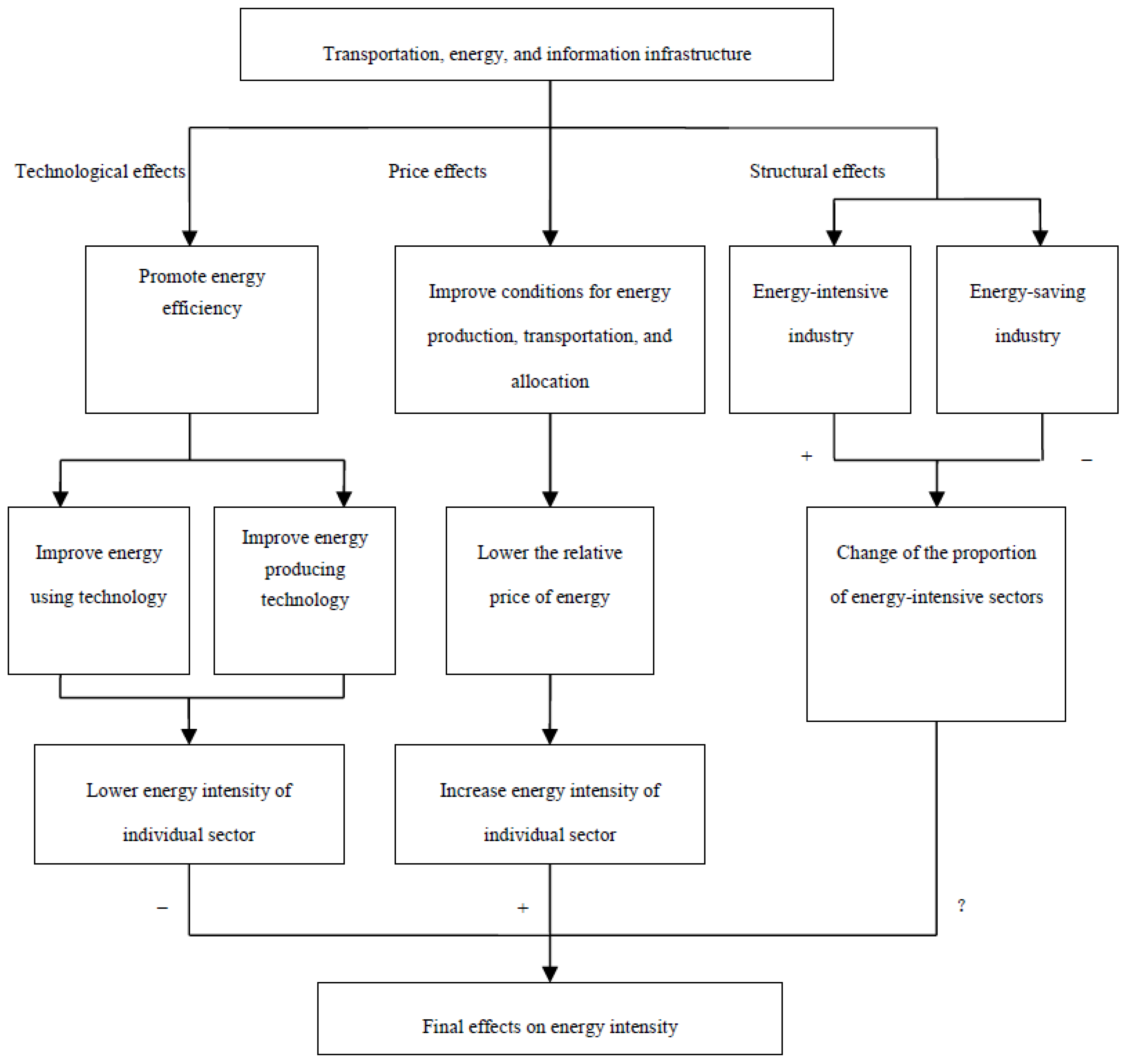
The critical problem is how does infrastructure affect energy intensity indirectly? We think that there are at least three kinds of effects: (1) technological effects, (2) price effects, and (3) structural effects. First, public infrastructure is beneficial in promoting the diffusion of technology. For example, transportation and information infrastructure speed up technology diffusion and then promote technological progress. Additionally, good public infrastructure also accelerates the inflow of foreign direct investment [51], which is beneficial for the technological progress of the host country [3,52], and decreases energy intensity. Second, good public infrastructure improves the conditions for energy production and transportation (i.e., decreasing the number of force majeure events and reducing cost of energy transport), which then lowers the price of energy. Although China keeps energy prices under tight control, the controlled price is usually based on the actual cost of energy. Good public infrastructure, such as natural gas pipelines, high voltage transmission lines, highways, and high-speed railways, has a substantial negative effect on energy prices and could lower energy costs. In theory, higher energy prices can push economic agents to save energy [53], or induce energy-saving innovations [54], and thus have a negative effect on energy intensity. Therefore, public infrastructure increases energy intensity indirectly through the channel of price effects. Third, in general, it is believed that well-developed transportation infrastructure will increase the proportion of the logistics industry in the overall economy [55], and modern information infrastructure will increase the proportion of the information industry in the overall economy [56]. Because the logistics industry is energy-intensive, while the information industry is energy-saving, the final effects of the increase of both kinds of infrastructure on energy intensity depend on the proportional growth of each sector. Figure 1 shows the impact public infrastructure mechanisms have on energy intensity through different effects.

The above figure shows that public infrastructure has a negative impact on energy intensity caused by technological effects and a positive impact caused by price effects. In addition, public infrastructure can also influence energy intensity through structural effects, but the direction of influence depends on the type of infrastructure. It is difficult to measure the specific influence quantitatively due to the lack of detailed data. Therefore, although we know public infrastructure influences energy intensity, we cannot determine the direction of the final effects.

However, we think the technological effects are the relatively more important effects. That is to say, the final effects will be negative or will eventually become negative once the scale of infrastructure reaches a certain level. We offer the following three reasons for our stance: first, technological effects will strengthen along with an increase in public infrastructure for its network effect; second, empirical literature found that energy intensity is less influenced by energy prices in China [9,57,58]. (There are at least two reasons for this phenomenon. One reason is that China is still in the middle stage of industrialization, and growth in energy consumption has outpaced the growth in energy supply, so the energy demand is rigid [58]. Another reason is that energy prices in China are mainly controlled by state-owned enterprises [7], and do not fully reflect scarcity of energy resources, environmental degradation, and imbalances in domestic demand and supply [8].), and the positive effects on energy intensity through the price effects will also be insignificant; and third, the influence of negative technological effects is wider than the influence of positive structural effects, because the former effects could influence all industries and sectors while the latter effects could only affect several individual sectors. Therefore, we propose that public infrastructure has a significant impact on energy intensity.

3. Methodology, Variables, and Model Specification

3.1. Methodology

In this paper, we adopt a PSTR model developed by Gonzalez et al. [59] and further improved by Fouquau et al. [60]. The PSTR model was first applied by González et al. (2005) to examine the effect of capital market imperfections on investment. This methodology has been commonly used in finance [61] and recently, in energy and environmental economics [62,63,64,65]. However, the public infrastructure–energy intensity relationship has not been studied from this perspective. After estimating a PSTR model of the income relationship of energy intensity and electricity consumption, Destais et al. [66] and Heidari et al. [67] summarize the four main advantages of this type of model. First, it allows the regression coefficients to change for each of the provinces in the panel along with time, thereby providing more consistent estimators. Second, PSTR modelling enables a smooth rather than an abrupt transition between extreme regimes, which is a more flexible and reliable framework. Third, the threshold value is not given a priori, but is calculated in the model. Finally, as infrastructure is also added as an explanatory variable, its impact on energy intensity is easy to measure. Capturing non-linearities and regime switching in this way makes the PSTR a good tool for the study of the public infrastructure–energy intensity relationship.

In a PSTR model, regression coefficients can take on a small number of different values depending on the value of another observable variable. Interpreted differently, the observations in the panel are divided into a small number of homogeneous groups or ‘regimes’, with different coefficients in different regimes. The basic PSTR model with two extreme regimes is defined as follows:

$$y_{it}={\mu }_i+{\beta }_0{x}_{it}+{\beta }_1{x}_{it}g(q_{it};\gamma ,c)+u_{it}$$

(1)

for i = 1,2,……N, and t = 1,2,……T, where N and T denote the cross-section and time dimensions of the panel respectively. y_it is an explained variable, x_it is a k-dimensional vector of time-varying explanatory variables, μ_i represents the individual fixed effects, and u_it represents the errors. q_it is a transition variable, γ is the slope parameter, c is the location parameter, and β₀ and β₁ are the regression coefficients. The transition function g(·) is a continuous function of the observable transition variable q_it and is normalized to be bounded between 0 and 1. The transition function is defined by Granger and Terasvirta [68] and Terasvirta [69] using the logistic specification as follows:

$$g(q_{it};\gamma ,c)={\left(1+\exp (-\gamma {\displaystyle \prod _{j=1}^m(q_{it}-c_j)}\right))}^{-1}, \gamma >0,c_1\le c_2\le \cdots c_m$$

(2)

where c_j is a location parameter, m is the number of location parameters, and the slope parameter γ determines the smoothness of the transition. The restrictions in the function are imposed only for identification purposes.

In the above PSTR model, the regression coefficients consist of the linear element β₀ and nonlinear element β₁·g(·) and fluctuate between β₀ and β₀ + β₁ as the threshold variable q_it increases, where the fluctuation is centered around c_j. Compared to a threshold model, a special characteristic of a PSTR model is that it allows for the regression coefficients to switch gradually when observations move from one group to another group. This assumption is more realistic, prompting a growing interest in the PSTR model.

3.2. Variables and Data Sources

3.2.1. Dependent Variable

This paper uses energy intensity (EI) as the dependent variable, which measures the energy efficiency of an economy and is calculated as units of energy per unit of GDP. It is given below in Equation (3) [4].

$$E{I}_{it}=\frac{TE{C}_{it}}{GD{P}_{it}}$$

(3)

where TEC_it denotes total energy consumption of province i at time t and GDP_it denotes real gross product of province i at year t using 2001 as the base year.

3.2.2. Explanatory Variables

This paper uses public infrastructure as an explanatory variable, which refers to public physical and organizational infrastructure needed for the operation of a society or enterprise, such as roads, electrical grids, or telecommunications [25,70]. Considering the importance and data availability of various types of infrastructure in China, we used the stock of transportation infrastructure (STI), energy infrastructure (SEI), and information infrastructure (SII) as the proxy variable of public infrastructure. The stock of these three kinds of infrastructure are measured by the density of highways above class II, the density of electrical grids, and the density of mobile phone exchange capacity, respectively. They are given below.

$$ST{I}_{it}=\frac{w_{LOE}LO{E}_{it}+w_{LOH1}LOH{1}_{it}+w_{LOH2}LOH{2}_{it}}{AO{P}_i}$$

(4)

where LOE_it, LOH1_it, and LOH2_it denote the length of expressway, the length of class I highway, and the length of class II highway of province i at year t, respectively. AOP_i denotes the area of province i. w_LOE, w_LOH1 and w_LOH2 are the weights of different kinds of highway which depend on the road’s capacity [71,72].

$$SE{I}_{it}=\frac{w_{LOPL1}LOPL{1}_{it}+w_{LOPL2}LOPL{2}_{it}+w_{LOPL3}LOPL{3}_{it}+w_{LOPL5}LOPL{5}_{it}}{AO{P}_i}$$

(5)

where LOPL1_it, LOPL2_it, LOPL3_it, and LOPL5_it represent the length of 110kV power line, the length of 220 kV power line, the length of 330 kV power line, and the length of 500kV power line of province i at year t respectively. AOP_i denotes the area of province i. w_LOPL1, w_LOPL2, w_LOPL3 and w_LOPL5 are the weights of the different kinds of power line which depend on their transmission and distribution capacity [71,72].

$$SI{I}_{it}=\frac{ME{C}_{it}}{AO{P}_i}$$

(6)

where MEC_it represents mobile phone exchange capacity of province i at year t. AOP_i denotes the area of province i.

3.2.3. Control Variables

Besides explanatory variables, we also used industry structure (IND), real income per capita (YPC), and provincial energy endowment (EE) as control variables following Ang [73], Greening et al. [74], Hubler and Keller [49], and Jiang and Ji [4]. Industry structure is measured in the proportion of secondary industry. Real income per capita is computed using 2001 as the base year and provincial energy endowment is measured in the ratio of provincial energy production to national energy production.

3.2.4. Transition Variables

What determines the size of the impact of specific infrastructure on energy intensity? There are at least two factors which could affect the shape of the infrastructure/energy intensity relationship: the stock of the specific infrastructure itself and the stock of information infrastructure. As such, we use these two factors as transition variables in this paper.

Transportation infrastructure, energy infrastructure, and information infrastructure are all typical network capital with economies of scale and network externality [25,75]. In other words, the effect of public infrastructure on energy intensity will change when the infrastructure stock increases gradually, and the final effect is nonlinear. In terms of network externality, once infrastructure stock reaches a critical level, its impact on energy intensity will rapidly switch from one equilibrium to another equilibrium [76].

Another factor thought to play a major role in determining the shape of the infrastructure–energy intensity relationship is the stock of information infrastructure, which could expand the impact of information and communication technologies (ICT hereafter). In one aspect, ICT could promote the operational and management efficiency of the infrastructure network, and then strengthen the effect of infrastructure on energy intensity [77]. In another aspect, ICT could also promote infrastructure-use efficiency through providing information and guidelines to the users of the infrastructure system [40].

3.2.5. Data Sources

The panel dataset is yearly and covers the period from 2001 to 2016 for 30 Chinese provincial regions. Tibet, Hong Kong, Macau and Taiwan are excluded due to data constraints. The data on the length of highways above class II, the capacity of mobile phone exchange, the region area, the share of secondary industry and gross domestic product of the 30 provinces were taken from the China Statistical Yearbook [78]. The data on the length of power line above 110 kV for the 30 provinces were taken from the China Electrical Yearbook [79]. Data on energy consumption and production of the 30 provinces were taken from China Energy Yearbook [80]. Weights used in Equations (4) and (5) were taken from Wang and Bi [72]. Based on the above data and Equations (3) to (6), we calculate the values of all variables used in this paper. All variables are expressed in natural logarithms.

Table 1. Descriptive statistics.

Variable	Obs	Mean	Std. Dev.	Min	Max	Description	Unit
lnEI	480	0.3258	0.4977	−0.7869	1.6060	energy intensity	tce per 104 yuan
lnSTI	480	5.3913	1.2310	1.6133	7.8635	stock of transportation infrastructure	km per 104 km2
lnSEI	480	7.7905	1.0809	4.2513	10.0917	stock of energy infrastructure	km per 104 km2
lnSII	480	5.0764	1.6177	0.1864	8.9672	stock of information infrastructure	subscribers per km2
lnIND	480	3.8099	0.1995	2.9581	4.0783	industry structure	%
lnYPC	480	0.5771	0.6884	−1.2096	2.1786	yield per capita	104 yuan
lnEE	480	0.3553	1.5485	−4.4619	3.4812	energy endowment	%

Notes: If prices are involved, the data is at 2001 constant price. For structure variables, the current year’s price is adopted.

reports the descriptive statistics for all variables.

3.3. Model Specifications

In accordance with the previous discussion, we assumed that the nonlinear relationship between public infrastructure and energy intensity depends on the scale of infrastructure stock. The basic equation is specified as follows:

$$\begin{array}{ll}\ln E{I}_{it}=& {\mu }_i+{\beta }_1\ln IN{D}_{it}+{\beta }_2\ln YP{C}_{it}+{\beta }_3\ln E{E}_{it}+{\beta }_4\ln IN{F}_{it}\\ & +{\beta }_5\ln IN{F}_{it}\cdot g(q_{it};\gamma ,c)+u_{it}\end{array}$$

(7)

where lnEI, lnIND, lnYPC, lnEE, and lnINF denote the natural logarithm values of EI, IND, YPC, EE, and INF. q_it is a transition variable. γ is the slope parameter, c is the location parameter and u_it represents the errors. The stock of transportation infrastructure (STI), energy infrastructure (SEI), and information infrastructure (SII) are used as the proxy variables of INF, respectively, and the specific infrastructure stock itself is used as the transition variable. Furthermore, information infrastructure stock (SII) will be used as a transition variable while STI and SEI are used as proxy variable of INF.

There are two problems that need to be solved before the estimation of Equation (7), namely, testing the linearity hypothesis of the model and choosing the proper value of m in Equation (2).

The PSTR model (Equation (7)) can be reduced to a linear model by imposing either γ = 0 or β₅ = 0. Therefore, testing the linearity hypothesis of model (Equation (7)) is equivalent to testing the null hypotheses as follows:

$$H_0:\gamma =0; or {H^{\prime }}_0:{\beta }_5=0$$

(8)

However, the associated tests are nonstandard because under either null hypothesis, the PSTR model contains the unidentified nuisance parameter c. This problem was first studied by Davies [81]. Luukonen et al. [82], Andrews and Ploberger [83], and Hansen [84] later proposed alternative solutions in the time series context, while Gonzalez et al. [59] proposed a solution in the panel data context. We follow Luukonen et al. [82] and Gonzalez et al. [59], and test the linearity hypothesis of the model using the null hypothesis H₀:γ = 0. To circumvent the identification problem, we replaced g(q_it; γ,c) in Equation (7) by its first-order Taylor expansion around γ = 0. After reparameterization, this leads to the following auxiliary regression equation:

$$\begin{array}{ll}\ln E{I}_{it}=& {\mu }_i+{\beta }_1\ln IN{D}_{it}+{\beta }_2\ln YP{C}_{it}+{\beta }_3\ln E{E}_{it}+{\beta }_4\ln IN{F}_{it}\\ & +{\beta }_1^{*}\ln IN{F}_{it}\cdot q_{it}+\cdots +{\beta }_m^{*}\ln IN{F}_{it}\cdot q_{it}^m+u_{it}^{*}\end{array}$$

(9)

According to the definition of the Taylor expansion, the parameter vectors β₁^*,…, β_m^* are multiples of γ. Consequently, testing the null hypothesis H₀:γ = 0 in Equation (8) is equivalent to testing the null hypothesis H_0′:β₁ ^* =…= β_m^* = 0 in Equation (9). This null hypothesis could be conveniently tested by a Lagrange multiplier test (LM). To define the LM statistics, we follow Mehrara et al. [85] in the following strategy: considering SSR₀ as the sum of the squares of panel errors in the null hypothesis H_0′ and SSR₁ as the sum of the squares of panel errors in Equation (9), the LM statistic is equal to the following:

$$LM=\left(\left(SS{R}_0-SS{R}_1\right)/k\cdot m\right)/\left(SS{R}_0/\left(T\cdot N-N-k\cdot m\right)\right)$$

(10)

where k refers to the number of explanatory variables, m is the number of location parameters, and N and T denote the cross-section and time dimensions of the panel, respectively. Under the null hypothesis, the LM statistic (Equation (10)) is asymptotically distributed as a chi-squared distribution with k·m degrees of freedom and the corresponding F statistic as the distribution F (k·m, T·N-N-k·m).

Another problem is the selection of an appropriate value for m, i.e., the number of location parameters. In practice, it is usually enough to consider m = 1 or m = 2, as these values allow for commonly encountered types of variations in the parameters [59]. Granger and Terasvirta [68] and Terasvirta [69] proposed a sequence of tests for choosing between m = 1 or m = 2 in similar studies. Applied to the present situation, this testing sequence reads as follows: using the auxiliary regression Equation (9) with m = 3, test null hypothesis H_00′: β₁^* = β₂^* = β₃^* = 0. If it is rejected, test H_03′: β₃^* = 0, H_02′: β₂^* = 0|β₃^* = 0 and H_01′: β₁^* = 0|β₂^* = β₃^* = 0. According to Terasvirta [69], if m = 2, then H_02′ will be rejected more strongly than H_03′ and H_01′. For m = 1, the situation is just the opposite. Therefore, we can select m = 2 if the rejection of H_02′ is the strongest. Otherwise, we should select m = 1.

Because the null hypothesis H_0′ contains the unknown parameter m, we first selected the proper value of m following the above testing sequence and then tested the linearity hypothesis of the models with the determined value for m.

Model 1 to Model 5 are described in the Appendix A. According to

Table 2. Linearity tests for selecting m.

Model (Explanatory Variable/Transition Variable)	H00′		H03′		H02′		H01′
	LM	p-Value	LM	p-Value	LM	p-Value	LM	p-Value
Model 1 (STI/STI)	40.7879	0.0000	0.7203	0.3901	9.5112	0.0020	31.2356	0.0000
Model 2 (STI/SII)	40.6435	0.0000	15.9915	0.0000	24.7144	0.0000	0.8299	0.3693
Model 3 (SEI/SEI)	21.7359	0.0000	0.6153	0.4328	3.9636	0.0465	17.3272	0.0000
Model 4 (SEI/SII)	62.6728	0.0000	10.9015	0.0000	48.4463	0.0000	5.0364	0.0248
Model 5 (SII/SII)	33.4464	0.0000	2.6352	0.1045	0.3203	0.5714	30.6814	0.0000

, all the null hypotheses H_00′ are strongly rejected, showing evidence of a nonlinear relationship among them. Rejection of H_01′ is the strongest in Model 1, Model 3, and Model 5, suggesting that these three models are the PSTR models with m = 1. In addition, the rejection of H_02′ is the strongest in Model 2 and Model 4. Thus, the PSTR models with m = 2 are chosen for Model 2 and Model 4.

4. Results

We estimate all five PSTR models described in the Appendix A using the non-linear square method and report the estimated results in

Table 3. Estimation results of PSTR models.

Model (Explanatory Variable/Transition Variable)	Model 1 (STI/STI)	Model 2 (STI/SII)	Model 3 (SEI/SEI)	Model 4 (SEI/SII)	Model 5 (SII/SII)
γ	15.5432 (18.5043)	0.2869 (0.1823)	2.7773 (1.9942)	0.9699 ** (0.4493)	3.9383 (2.7765)
c1	3.9604 *** (0.0819)	10.0443 *** (2.0140)	4.8595 *** (0.4553)	7.6793 *** (0.1083)	7.8414 *** (0.1829)
c2		2.1483 *** (0.4146)		1.7189 *** (0.2075)
lnSTI	−0.0034 * (0.0019)	−0.0025 * (0.0016)
lnSTI·g(lnSTI)	−0.0876 *** (0.0245)
lnSTI·g(lnSII)		−0.3394 * (0.1819)
lnSEI			0.0323 *** (0.0829)	0.1339 *** (0.0329)
lnSEI·g(lnSEI)			0.0805 * (0.0492)
lnSEI·g(lnSII)				−0.0281 *** (0.0060)
lnSII					−0.0963 *** (0.0197)
lnSII·g(lnSII)					−0.0728 *** (0.0163)
lnIND	0.2293 *** (0.0339)	0.6361 *** (0.0517)	0.6555 *** (0.0481)	0.5628 *** (0.0509)	0.3209 *** (0.0168)
lnYPC	−0.2685 *** (0.0304)	−0.3936 *** (0.0331)	−0.4466 *** (0.0314)	−0.4733 *** (0.0289)	−0.1660 *** (0.0326)
lnEE	0.0768 *** (0.0108)	0.0146 (0.0127)	0.0234 * (0.0126)	0.0185 (0.0129)	0.0859 *** (0.0108)
N	480	480	480	480	480

Notes: ***, ** and * denote significance at the 1%, 5% and 10% levels, respectively; standard errors are given in brackets.

. The estimated slope parameters are relatively small in all models, implying that there is a continuum of conditions between two regimes. That is to say, the transition from one regime to another is smooth. We also employed a quadratic polynomial model to explore the nonlinear relationship between public infrastructure and energy intensity. The results are presented in

Table A1. Estimation results of quadratic polynomial models.

Variable	Model 6	Model 7	Model 8	Model 9	Model 10
lnSTI	0.2620 **	0.0722
	(0.1031)	(0.0895)
lnSEI			0.5217 **	0.1619
			(0.2050)	(0.1125)
lnSII					0.2119 ***
					(0.0748)
(lnSTI)2	−0.0313 ***
	(0.0100)
lnSTI *lnSII		−0.0134 *
		(0.0072)
(lnSEI)2			0.0319 **
			(0.0122)
lnSEI *lnSII				−0.0052
				(0.0072)
(lnSII)2					−0.0130 ***
					(0.0044)
IND	0.2437 *	0.2706 **	0.2037	0.2534 *	0.1733
	(0.1345)	(0.1213)	(0.1374)	(0.1283)	(0.1434)
YPC	−0.3018	−0.2818	−0.3045 *	−0.3196 *	−0.3602 **
	(0.1896)	(0.2071)	(0.1526)	(0.1677)	(0.1703)
EE	0.0383 **	0.0509 **	0.0388 **	0.0540 **	0.0352 **
	(0.0164)	(0.0207)	(0.0158)	(0.0204)	(0.0152)
cons	−1.0182 *	−0.7119	−2.4368 **	−1.5823 *	−0.8382
	(0.5875)	(0.6173)	(0.9366)	(0.8552)	(0.5273)
N	480	480	480	480	480
FE	Y	Y	Y	Y	Y
Wald test	9.82 ***	3.42 *	6.83 **	0.53	8.76 ***
Adj.R2	0.8565	0.8423	0.8559	0.8435	0.8600

Notes: (1) ***, ** and * denote significance at the 1%, 5% and 10% levels, respectively; standard errors are given in brackets. (2) Energy intensity is the explained variable in all five models used to explore the nonlinear relationship between public infrastructure and energy intensity. (3) Model 6 uses transportation infrastructure (lnSTI) and quadratic term of lnSTI as explanatory variables. Model 7 uses transportation infrastructure (lnSTI) and interaction term of lnSTI and information infrastructure (lnSII) as explanatory variables. Model 8 uses energy infrastructure (lnSEI) and quadratic term of lnSEI as explanatory variables. Model 9 uses energy infrastructure (lnSEI) and interaction term of lnSEI and lnSII as explanatory variables. Model 10 uses lnSII and quadratic term of lnSII as explanatory variables. (4) Null hypothesis of Wald test is that the coefficient of quadratic term in the model is equal to zero.

in the Appendix A. According to the Wald test in Table A1, linearity hypotheses are rejected in all five models except Model 9, implying that it is more proper to take the nonlinearity relationship into account. In general, the nonlinear effect of public infrastructure on energy intensity in PSTR models tends to be quite similar to the results of quadratic polynomial models in most cases, which confirms that the PSTR is a good approximation of the quadratic fixed effects model. Indeed, the inclusion of quadratic and interaction terms might be well suited to model U-shaped relations, but fails to account properly for more complex nonlinear effects that could be well modeled by the PSTR approach [86]. Therefore, in the following paragraphs we will focus on the estimation results of the PSTR approach.

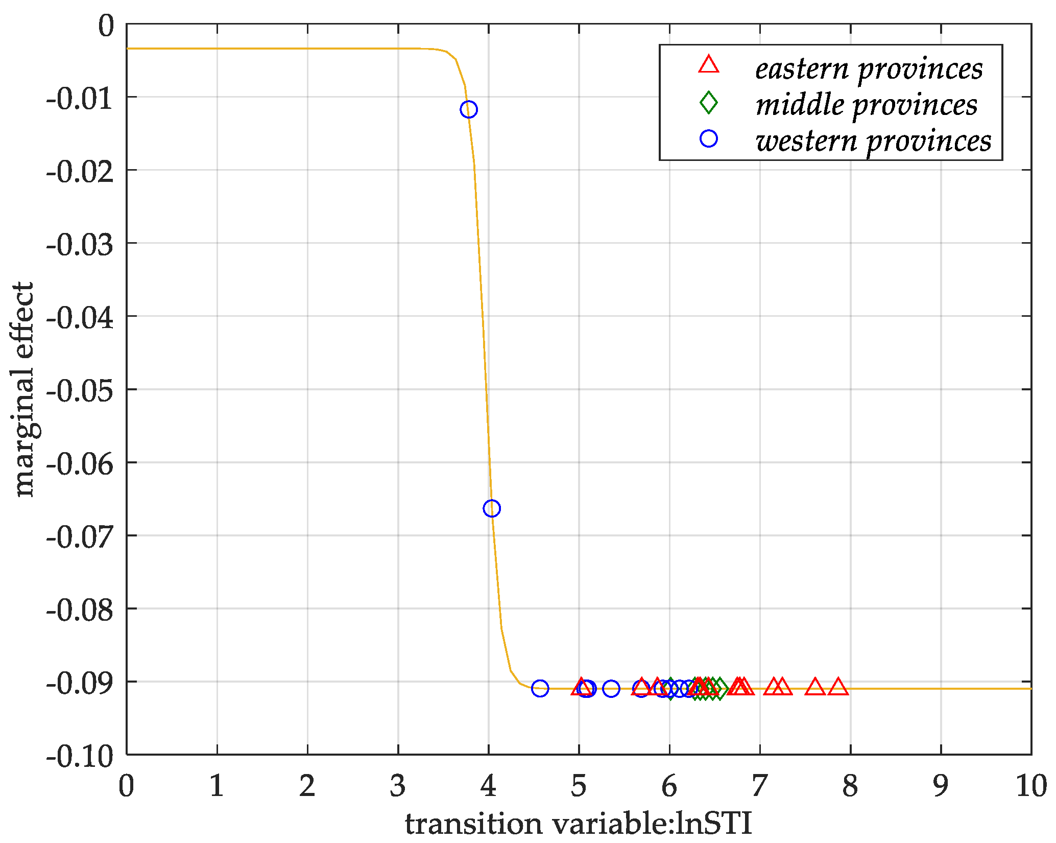
Model 1 and Model 2 of Table 3 show the results when public infrastructure is proxied by transportation infrastructure and the transition variable is proxied by transportation and information infrastructure, respectively. As shown in Model 1, there is a significantly negative relationship between transportation infrastructure and energy intensity, since the estimated coefficients of lnSTI are significantly negative (−0.0034 and −0.091) in the two regimes. These results suggest that as the stock of transportation infrastructure rises, energy intensity decreases slowly in the early stage of the transportation development. In the later stage, energy intensity then rapidly decreases after the level of transportation infrastructure exceeds approximately 52.5 km per 10⁴ km² (estimated location parameter is 3.9604). These results are similar to those of Rudra [87] and Guo and Zhang [88]. They found that investment in transportation infrastructure could enhance energy efficiency, but they did not take a nonlinearity relationship between transportation infrastructure on energy intensity into consideration. The marginal effect (see details in the Appendix A) of transportation infrastructure on energy intensity using transportation infrastructure as a transition variable is shown as the yellow line in Figure 2. The final effects of transportation infrastructure on the energy intensity of 30 provinces in 2016 are also shown in Figure 2. The provinces are divided into eastern, middle, and western provinces (see details in

Table A2. The stock of three types of public infrastructure in 30 provinces in 2016.

	Province	Transportation Infrastructure	Energy Infrastructure	Information Infrastructure
Eastern Provinces	Beijing	7.151	9.212	8.043
	Fujian	6.311	8.603	6.498
	Guangdong	6.774	8.881	7.108
	Hainan	5.865	8.174	6.162
	Hebei	6.429	8.851	6.442
	Heilongjiang	5.024	7.412	5.225
	Jiangsu	7.245	9.574	6.991
	Jilin	5.691	8.080	5.366
	Liaoning	6.336	8.883	6.113
	Shandong	6.823	8.953	6.739
	Shanghai	7.864	10.090	8.940
	Tianjin	7.609	9.447	7.762
	Zhejiang	6.747	9.186	7.065
Middle Provinces	Anhui	6.397	8.753	6.472
	Henan	6.556	8.732	6.649
	Hubei	6.476	8.700	6.186
	Hunan	6.010	8.208	5.845
	Jiangxi	6.279	8.239	5.566
	Shanxi	6.337	8.749	5.828
Western Provinces	Chongqing	6.213	8.603	6.195
	Gansu	5.068	7.222	4.385
	Guangxi	5.686	7.924	5.419
	Guizhou	5.997	8.094	5.665
	Neimenggu	4.569	7.169	4.047
	Ningxia	6.110	7.974	5.367
	Qinghai	4.035	6.047	2.900
	Shannxi	5.923	7.987	5.595
	Sichuan	5.354	7.966	5.834
	Xinjiang	3.781	6.013	3.685
	Yunnan	5.095	8.009	5.021

Notes: The stocks of the three types of public infrastructure in the 30 provinces were calculated according to Equation (4) to (6), and the original data were taken from China Statistical Yearbook, China Electrical Yearbook, and China Energy Yearbook. All variables are expressed in natural logarithm. The units of the stocks of transportation infrastructure, energy infrastructure and information infrastructure are km per 10⁴ km², km per 10⁴ km² and subscribers per km² respectively.

in the Appendix A). According to Figure 2, except for two western provinces, Qinghai and Xinjiang, transportation infrastructure stocks have already exceeded the threshold value in the remaining provinces, which implies that these provinces will remain in the high-impact regime when the stock of transportation infrastructure increases.

The two threshold parameters in Model 2 are estimated to be approximately 8.57 subscribers per km² (estimated location parameter is 2.1483) and 23,024.17 subscribers per km² (estimated location parameter is 10.0443). It is implied that when the transition variable (information infrastructure) grows, the marginal effect of transportation infrastructure on energy intensity will gradually decrease from 0.3419 to 0.0025 in absolute value after the level of information infrastructure stock exceeds the smaller threshold value. Then, it will gradually increase to 0.3419 again when information infrastructure stock exceeds the bigger threshold value. These findings provide an interpretation of the different influences of ICT infrastructure found by Abdolrasoul and Roghayeh [89]. They observed that information infrastructure strengthens the impact of transportation infrastructure on energy intensity in some countries, while it weakens the previously mentioned impact in other countries. Furthermore, both coefficients of the transportation infrastructure and transition variable are significantly negative in Model 2, implying that the impact of transportation infrastructure on energy intensity is still negative when using information infrastructure as the transition variable. The marginal effect of transportation infrastructure and the impacts of 30 provinces in 2016 are presented in Figure 3. According to Figure 3, the information infrastructure stocks of these provinces are all between the two threshold values, implying that the impact of transportation infrastructure on energy intensity tends to increase as information infrastructure increases.

Model 3 and Model 4 of Table 3 show the results when public infrastructure is proxied by energy infrastructure and the transition variable is proxied by energy and information infrastructure respectively. As shown in Model 3, there is a significantly positive relationship between energy infrastructure and energy intensity, which is similar to the findings of Wang et al. [90]. However, in our model, we took the nonlinear relationship into consideration and found that the influence of energy infrastructure on energy intensity gradually switches from low impact regime (0.0323) to high impact regime (0.1128). This change occurs when the energy infrastructure stock exceeds the threshold value of 128.96 km per 10⁴ km² (estimated location parameter is 4.8595). The marginal effects of energy infrastructure on the 30 provinces’ energy intensity are shown in Figure 4. According to Figure 4, the energy infrastructure stocks of all provinces have already exceeded the threshold value, implying that the impact of energy infrastructure on energy intensity has already switched from a low impact regime to a high impact regime.

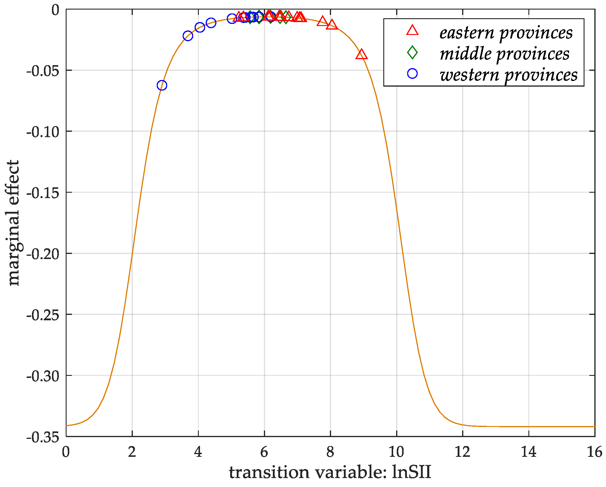
Considering Model 4, which uses the stock of information infrastructure as the transition variable, the results clearly demonstrate a nonlinear relationship. The two threshold parameters in Model 4 are estimated to be approximately 5.58 subscribers per km² (estimated location parameter is 1.7189) and 2163.11 subscribers per km² (estimated location parameter is 7.6793). This result implies that information infrastructure could make energy infrastructure more efficient and thus strengthens the positive impact of the energy infrastructure on energy intensity, which is consistent with Laitner’s results [77]. But when the information infrastructure stock exceeds the larger threshold value, the positive influence of the energy infrastructure on energy intensity will gradually decrease to 0.1048, which is consistent with the findings of Wang et al. [90]. Our results provide an integrated interpretation to the different impacts of energy infrastructure on energy intensity as described by Laitner and Wang et al. Figure 5 clearly shows the nonlinear impact of energy infrastructure on energy intensity and the smooth switching from one regime to another regime as information infrastructure increases. Additionally, according to Figure 5, the information infrastructure stock in three eastern provinces (i.e., Shanghai, Beijing and Tianjin) has already surpassed the larger threshold value, thus weakening the positive influence of energy infrastructure on energy intensity. However, the information infrastructure in the remaining provinces remains at a relatively lower level and should be improved in the future.

The results of Model 5 show that there is a significantly negative relationship between information infrastructure on energy intensity, since the estimated coefficients of information infrastructure are both significantly negative (−0.0963 and −0.1691) in the two regimes, which is similar to Zhou et al. [13]. These results suggest that as information infrastructure stock rises, energy intensity slowly decreases during the early stage of information infrastructure development, and then rapidly decreases during the later stage, after the level of information infrastructure exceeds 2543.76 subscribers per km² (estimated location parameter is 7.8414). Figure 6 shows the marginal effect of information infrastructure on energy intensity as information infrastructure grows. In Figure 6, we also presented the influences of the 30 provinces. According to Figure 6, the information infrastructure stocks are still below the threshold value, except for three eastern provinces (i.e., Shanghai, Beijing and Tianjin). This means that improving the information infrastructure in most of the provinces would reduce the energy intensity.

In addition, the estimated coefficients of industry structure and energy endowment, are positive in all the models, although the coefficients of energy endowment in Model 2 and Model 4 are insignificant, implying that energy intensity will increase when the proportion of secondary industry or the ratio of provincial energy production to national energy production increases, which is consistent with economic theory and the existing literature [4,49]. The significantly negative coefficients of income per capita mean that energy intensity will decrease when income per capita increases, which is consistent with Greening et al. [74].

5. Conclusions and Policy Implications

Using a panel smooth transition regression model, this paper empirically assessed the nonlinear relationship between public infrastructure and energy intensity in 30 Chinese provinces from 2001 to 2016. Noticing that different types of public infrastructure may have different impact patterns on energy intensity, we used three types of public infrastructure (i.e., transportation, energy, and information infrastructure) as the proxy variables, respectively. The results show that there exists a clear nonlinear relationship between energy intensity and public infrastructure.

The main conclusions are as follows. First, transportation infrastructure has a significantly negative effect on energy intensity, and this negative effect could be gradually strengthened when the transportation infrastructure stock exceeds the threshold value. Adversely, energy infrastructure has a significantly positive effect on energy intensity, and this positive effect will be gradually strengthened during the development of energy infrastructure. Second, the development of information infrastructure could not only strengthen its own significantly negative effect on energy intensity, but it could also promote the negative effect of transportation infrastructure on energy intensity. Moreover, the positive impact of energy infrastructure on energy intensity gradually decreases when the stock of information infrastructure surpasses the larger threshold value. Finally, different types of public infrastructure have different nonlinear impact patterns on energy intensity, which may explain why existing studies on the nexus between public infrastructure and energy intensity appear to exhibit diverse and dissimilar results.

The above results can provide guidance on developing appropriate infrastructure and energy policies and reconcile the dilemma of economic growth, energy consumption, and environmental protection in China. The important policy implications of these conclusions are as follows: First, the findings suggest that policy makers could reduce energy intensity by accelerating the development of transportation infrastructure. Moreover, they could further strengthen the negative effect of transportation infrastructure on energy intensity in Xinjiang and Qinghai through the increase of transportation infrastructure investment, since the stock of transportation infrastructure is still below the threshold value in these two provinces. Second, policy makers could also reduce energy intensity by accelerating the development of information infrastructure. Furthermore, they could strengthen the negative effects of transportation infrastructure and information infrastructure on energy intensity and weaken the positive effect of energy infrastructure on energy intensity by increasing information infrastructure investment since the scale of information infrastructure in most of provinces is still below the threshold values. Finally, paying more attention to accelerating the development of information infrastructure in western provinces will be beneficial to strengthening the negative effects of public infrastructure on energy intensity, because western provinces are lagging behind the middle and eastern provinces in the construction of information infrastructure.

Although using transportation, energy and information infrastructure as proxy variables of public infrastructure correspondingly provides valuable insights, it has limitations, which should serve to stimulate further research. First, our research is limited to the sample data. Extending the study to evaluate other types of public infrastructure to confirm our findings and test the sensitivity of the results is one area where we could extend this study. Second, this paper could not provide more information about the relationship between energy intensity and aggregated measures of public infrastructure. In further research, we may consider building an aggregative indicator of public infrastructure using two methods. One is by using the principal components analysis method to aggregate different types of physical public infrastructure. The other is by calculating the capital stock of the different types of public infrastructure that could be aggregated directly. Then we can further analyze the nexus between energy intensity and aggregated public infrastructure.

References

- Wu, L.; Kaneko, S.; Matsuoka, S. Driving forces behind the stagnancy of China’s energy-related CO2 emissions from 1996 to 1999: The relative importance of structural change, intensity change and scale change. Energy Policy 2005, 33, 319–335. [Google Scholar] [CrossRef]
- Yang, L.; Yang, T. Energy consumption and economic growth from perspective of spatial heterogeneity: Statistical analysis based on variable coefficient model. Ann. Oper. Res. 2015, 228, 151–161. [Google Scholar] [CrossRef]
- Huang, J.; Du, D.; Tao, Q. An analysis of technological factors and energy intensity in China. Energy Policy 2017, 109, 1–9. [Google Scholar] [CrossRef]
- Jiang, L.; Ji, M. China’s Energy Intensity, Determinants and Spatial Effects. Sustainability 2016, 8, 544. [Google Scholar] [CrossRef]
- Zhao, X.; Ma, C.; Hong, D. Why did China’s energy intensity increase during 1998–2006: Decomposition and policy analysis. Energy Policy 2010, 38, 1379–1388. [Google Scholar] [CrossRef] [Green Version]
- Han, Y.; Fan, Y.; Jiao, L.; Yan, J.S.; Wei, Y.M. Energy structure, marginal efficiency and substitution rate: An empirical study of China. Energy 2007, 32, 935–942. [Google Scholar] [CrossRef]
- Li, K.; Lin, B. The nonlinear impacts of industrial structure on China’s energy intensity. Energy 2014, 69, 258–265. [Google Scholar] [CrossRef]
- Jiang, L.; Folmer, H.; Ji, M. The drivers of energy intensity in China: A spatial panel data approach. China Econ. Rev. 2014, 31, 351–360. [Google Scholar] [CrossRef]
- Yang, G.; Li, W.; Wang, J.; Zhang, D. A comparative study on the influential factors of China’s provincial energy intensity. Energy Policy 2016, 88, 74–85. [Google Scholar] [CrossRef]
- Zeng, L.; Xu, M.; Liang, S.; Zeng, S.; Zhang, T. Revisiting drivers of energy intensity in China during 1997–2007: A structural decomposition analysis. Energy Policy 2014, 67, 640–647. [Google Scholar] [CrossRef]
- Jiang, X.; Duan, Y.; Green, C. Regional disparity in energy intensity of China and the role of industrial and export structure. Resour. Conserv. Recycl. 2017, 120, 209–218. [Google Scholar] [CrossRef]
- Li, H.; Lo, K.; Wang, M.; Zhang, P.; Xue, L. Industrial Energy Consumption in Northeast China under the Revitalisation Strategy: A Decomposition and Policy Analysis. Energies 2016, 9, 549. [Google Scholar] [CrossRef]
- Zhou, X.; Zhou, D.; Wang, Q. How does information and communication technology affect China’s energy intensity? A three-tier structural decomposition analysis. Energy 2018, 151, 748–759. [Google Scholar] [CrossRef]
- Voigt, S.; Cian, E.D.; Schymura, M.I.; Verdolini, E. Energy intensity developments in 40 major economies: Structural change or technology improvement? Energy Econ. 2014, 41, 47–62. [Google Scholar] [CrossRef] [Green Version]
- Elliott, R.; Sun, P.; Zhu, T. The direct and indirect effect of urbanization on energy intensity: A province-level study for China. Energy 2017, 123, 677–692. [Google Scholar] [CrossRef]
- Ma, B. Does urbanization affect energy intensities across provinces in China? Long-run elasticities estimation using dynamic panels with heterogeneous slopes. Energy Econ. 2015, 49, 390–401. [Google Scholar] [CrossRef]
- Yan, H. Provincial energy intensity in China: The role of urbanization. Energy Policy 2015, 86, 635–650. [Google Scholar] [CrossRef]
- Huang, J.; Du, D.; Hao, Y. The driving forces of the change in China’s energy intensity: An empirical research using DEA-Malmquist and spatial panel estimations. Econ. Model. 2017, 65, 41–50. [Google Scholar] [CrossRef]
- Tyutikov, V.V.; Smirnov, N.N.; Lapateev, D.A. Analysis of energy efficiency from the use of heat-reflective window screens in different regions of Russia and France. Procedia Eng. 2016, 150, 1657–1662. [Google Scholar] [CrossRef]
- Sequeira, T.; Santos, M. Education and Energy Intensity: Simple Economic Modelling and Preliminary Empirical Results. Sustainability 2018, 10, 2625. [Google Scholar] [CrossRef]
- Shi, Y.; Guo, S.; Sun, P. The role of infrastructure in China’s regional economic growth. J. Asian Econ. 2017, 49, 26–41. [Google Scholar] [CrossRef]
- World Bank. World Development Report 1994: Infrastructure for Development; Oxford University Press: Oxford, UK, 1994. [Google Scholar]
- Easterly, W.; Luis, S. The Limits of Stabilization: Infrastructure, Public Deficits, and Growth in Latin America. World Bank Publ. 2003, 42, 1139–1140. [Google Scholar]
- Sahoo, P.; Dash, R.K. Infrastructure development and economic growth in India. J. Asia Pac. Econ. 2009, 14, 351–365. [Google Scholar] [CrossRef]
- Duggal, V.G.; Saltzman, C.; Klein, L.R. Infrastructure and productivity: A nonlinear approach. J. Econom. 1999, 92, 47–74. [Google Scholar] [CrossRef]
- Romer, P.M. Increasing returns and long-run growth. J. Political Econ. 1986, 94, 1002–1037. [Google Scholar] [CrossRef]
- Barro, R.J. Government spending in a simple model of endogenous growth. J. Political Econ. 1990, 98, 103–125. [Google Scholar] [CrossRef]
- Hulten, C.R. Infrastructure, Externalities, and Economic Development: A Study of the Indian Manufacturing Industry. World Bank Econ. Rev. 2006, 20, 291–308. [Google Scholar] [CrossRef]
- Ansar, A.; Flyvbjerg, B.; Budzier, A. Does infrastructure investment lead to economic growth or economic fragility? Evidence from China. Oxf. Rev. Econ. Policy 2016, 32, 360–390. [Google Scholar] [CrossRef] [Green Version]
- Wiśnicki, B.; Chybowski, L.; Czarnecki, M. Analysis of the efficiency of port container terminals with the use of the Data Envelopment Analysis method of relative productivity evaluation. Manag. Syst. Prod. Eng. 2017, 25, 9–15. [Google Scholar] [CrossRef]
- Anna, M.; Raymond, J.; Adriana, R. Regional infrastructure investment and efficiency. Reg. Stud. 2018, 52, 1684–1694. [Google Scholar]
- Bankole, F.; Osei-Bryson, K.; Brown, I. The Impacts of Telecommunications Infrastructure and Institutional Quality on Trade Efficiency in Africa. Inf. Technol. Dev. 2015, 21, 29–43. [Google Scholar] [CrossRef]
- Mitra, A.; Sharma, C.; Veganzones-Varoudakis, M. Estimating impact of infrastructure on productivity and efficiency of Indian manufacturing. Appl. Econ. Lett. 2012, 19, 779–783. [Google Scholar] [CrossRef]
- Cho, Y.; Lee, J.; Kim, T.Y. The impact of ICT investment and energy price on industrial electricity demand: Dynamic growth model approach. Energy Policy 2007, 35, 4730–4738. [Google Scholar] [CrossRef]
- Wang, D.; Han, B. The impact of ICT investment on energy intensity across different regions of China. J. Renew. Sustain. Energy 2016, 8, 855–901. [Google Scholar] [CrossRef]
- Privitera, R.; La, R.D. Reducing Seismic Vulnerability and Energy Demand of Cities through Green Infrastructure. Sustainability 2018, 10, 2591. [Google Scholar] [CrossRef]
- Zhang, D.; Cao, H.; Wei, Y.M. Identifying the determinants of energy intensity in China: A Bayesian averaging approach. Appl. Energy 2016, 168, 672–682. [Google Scholar] [CrossRef]
- Burton, E. The compact city: Just or just compact? A preliminary analysis. Urban Stud. 2000, 37, 1969–2006. [Google Scholar] [CrossRef]
- Herrerias, M.J.; Cuadros, A.; Orts, V. Energy intensity and investment ownership across Chinese provinces. Energy Econ. 2013, 36, 286–298. [Google Scholar] [CrossRef] [Green Version]
- Giannopoulos, G.A. The application of information and communication technologies in transport. Eur. J. Oper. Res. 2004, 152, 302–320. [Google Scholar] [CrossRef]
- Howarth, R.B. Energy use in U.S. manufacturing: The impacts of the energy shocks on sectoral output, industry structure, and energy intensity. J. Energy Dev. 1989, 14, 175–191. [Google Scholar]
- Schipper, L.; Howarth, R.; Andersson, B. Energy Use in Denmark: An International Perspective. Natural Resour. Forum 1993, 17, 83–103. [Google Scholar] [CrossRef]
- Ang, B.W. Multilevel decomposition of industrial energy consumption. Energy Econ. 1995, 17, 265–270. [Google Scholar] [CrossRef]
- Zarnikau, J. A Note: Will Tomorrow’s Energy Efficiency Indices Prove Useful in Economic Studies? Energy J. 1999, 20, 139–145. [Google Scholar] [CrossRef]
- Boyd, G.A.; Roop, J.M. A note on the Fischer ideal index decomposition for structural change in energy intensity. Energy J. 2004, 25, 87–101. [Google Scholar] [CrossRef]
- Lescaroux, F. Decomposition of US manufacturing energy intensity and elasticities of components with respect to energy prices. Energy Econ. 2008, 30, 1068–1080. [Google Scholar] [CrossRef]
- Wang, C.; Liao, H.; Pan, S.Y.; Zhao, L.T.; Wei, Y.M. The fluctuations of China’s energy intensity: Biased technical change. Appl. Energy 2014, 135, 407–414. [Google Scholar] [CrossRef]
- Liao, H.; Fan, Y.; Wei, Y.M. What induced China’s energy intensity to fluctuate: 1997–2006? Energy Policy 2007, 35, 4640–4649. [Google Scholar] [CrossRef]
- Hubler, M.; Keller, A. Energy savings via FDI? empirical evidence from developing countries. Environ. Dev. Econ. 2009, 15, 59–80. [Google Scholar] [CrossRef]
- Karl, Y.; Chen, Z. Government expenditure and energy intensity in China. Energy Policy 2010, 38, 691–694. [Google Scholar]
- Sahoo, P. FDI in south Asia: Trends, policy, impact and determinants. Asian Dev. Bank Inst. Discuss. Pap. 2006, 56, 36–43. [Google Scholar]
- Keller, W. International technology diffusion. J. Econ. Lit. 2004, 42, 752–782. [Google Scholar] [CrossRef]
- Birol, F.; Keppler, J.H. Prices, technology development and the rebound effect. Energy Policy 2000, 28, 457–469. [Google Scholar] [CrossRef]
- Fisher-Vanden, K.; Jefferson, G.H.; Liu, H.M.; Tao, Q. What is driving China’s decline in energy intensity? Resour. Energy Econ. 2004, 26, 77–97. [Google Scholar] [CrossRef]
- Zhang, Z.; Figliozzi, M.A. A Survey of China’s Logistics Industry and the Impacts of Transport Delays on Importers and Exporters. Transp. Rev. 2010, 30, 179–194. [Google Scholar] [CrossRef] [Green Version]
- Hong, J.P.; Byun, J.F.; Kim, P.R. Structural changes and growth factors of the ICT industry in Korea: 1995–2009. Telecommun. Policy 2016, 40, 502–513. [Google Scholar] [CrossRef]
- Hang, L.; Tu, M. The impacts of energy prices on energy intensity: Evidence from China. Energy Policy 2007, 35, 2978–2988. [Google Scholar] [CrossRef]
- Song, F.; Zheng, X. What drives the change in China’s energy intensity: Combining decomposition analysis and econometric analysis at the provincial level. Energy Policy 2012, 51, 445–453. [Google Scholar] [CrossRef]
- González, A.; Terasvirta, T.; Dijk, D.V. Panel Smooth Transition Regression Model; No. 165; Working Paper Series; Quantitative Finance Research Centre, University of Technology: Sydney, Australia, 2005. [Google Scholar]
- Fouquau, J.; Ghislaine, D.; Hurlin, C. Energy demand models: A threshold panel specification of the kuznets curve. Appl. Econ. Lett. 2009, 16, 1241–1244. [Google Scholar] [CrossRef]
- Chang, T.; Chiang, G. Regime-switching effects of debt on real GDP per capita the case of Latin American and Caribbean countries. Econ. Model. 2011, 28, 2404–2408. [Google Scholar] [CrossRef]
- Bessec, M.; Fouquau, J. The non-linear link between electricity consumption and temperature in Europe: A threshold panel approach. Energy Econ. 2008, 30, 2705–2721. [Google Scholar] [CrossRef]
- Lee, C.C.; Chiu, Y.B. Electricity demand elasticities and temperature: Evidence from panel smooth transition regression with instrumental variable approach. Energy Econ. 2011, 33, 896–902. [Google Scholar] [CrossRef]
- Chiu, Y.B. Deforestation and the environmental Kuznets curve in developing countries: A panel smooth transition regression approach. Can. J. Agric. Econ. 2012, 60, 177–194. [Google Scholar] [CrossRef]
- Chai, J.; Xing, L.; Lu, Q.; Liang, T.; Kin, K.; Wang, S. The Non-Linear Effect of Chinese Financial Developments on Energy Supply Structures. Sustainability 2016, 8, 1021. [Google Scholar] [CrossRef]
- Destais, G.; Fouquau, J.; Hurlin, C. Economic Development and Energy Intensity: A Panel Data Analysis. In The Econometrics of Energy Systems; Girod, J., Bourbonnais, R., Keppler, J.H., Eds.; Palgrave Macmillan: Basingstoke, UK, 2007. [Google Scholar]
- Heidaria, H.; Katircioglu, S.T.; Saeidpour, L. Economic growth, CO2 emissions, and energy consumption in the five ASEAN countries. Electr. Power Energy Syst. 2015, 64, 785–791. [Google Scholar] [CrossRef]
- Granger, C.W.; Terasvirta, T. Modeling Nonlinear Economic Relationships; Oxford University Press: Oxford, UK, 1993. [Google Scholar]
- Terasvirta, T. Specification, estimation and evaluation of smooth transition autoregressive models. J. Am. Stat. Assoc. 1994, 89, 208–218. [Google Scholar]
- Fung, K.C.; Garcia-Herrero, A.; Iizaka, H.; Sin, A. Hard or soft? institutional reforms and infrastructure spending as determinants of foreign direct investment in China. Jpn. Econ. Rev. 2005, 56, 408–416. [Google Scholar] [CrossRef]
- Sanchez-Robles, B. Infrastructure Investment and Growth Some Empirical Evidence. Contemp. Econ. Policy 1998, 16, 98–108. [Google Scholar] [CrossRef]
- Wang, Z.; Bi, C. The impact of infrastructure investment on energy intensity: Empirical analysis based on provincial panel data. Stat. Inf. Forum 2012, 47, 45–51. (In Chinese) [Google Scholar]
- Ang, B.W. Is the energy intensity a less useful indicator than the carbon factor in the study of climate change? Energy Policy 1999, 27, 943–946. [Google Scholar] [CrossRef]
- Greening, L.A.; Greene, D.L.; Difiglio, C. Energy efficiency and consumption—the rebound effect—A survey. Energy Policy 2000, 28, 389–401. [Google Scholar] [CrossRef]
- Tapscott, D. The Digital Economy; Mc Graw-Hill: New York, NY, USA, 1996. [Google Scholar]
- Katz, M.L.; Shapiro, C. Systems Competition and Network Effects. J. Econ. Perspect. 1994, 8, 93–115. [Google Scholar] [CrossRef]
- Laitner, J.A.S. The Energy Efficiency Benefits and the Economic Imperative of ICT-Enabled Systems. In ICT Innovations for Sustainability. Advances in Intelligent Systems and Computing; Hilty, L., Aebischer, B., Eds.; Springer: Cham, Switzerland, 2015. [Google Scholar]
- National Bureau of Statistics of China. China Statistical Yearbook; China Statistics Press: Beijing, China, 2002–2017.
- The Editorial Board of China Electrical Yearbook. China Electrical Yearbook; China Electric Power Press: Beijing, China, 2002–2017. [Google Scholar]
- National Bureau of Statistics of China. China Energy Yearbook; China Statistics Press: Beijing, China, 2002–2017.
- Davies, R.B. Hypothesis testing when a nuisance parameter is present only under the alternative. Biometrika 1987, 74, 33–43. [Google Scholar]
- Luukkonen, R.; Saikkonen, P.; Teresavirta, T. Testing Linearity against Smooth Transition Autoregressive Models. Biometrika 1988, 75, 491–499. [Google Scholar] [CrossRef]
- Andrews, D.W.K.; Ploberger, W. Optimal Tests when a Nuisance Parameter is Present Only under the Alternative. Econometrica 1994, 62, 1383. [Google Scholar] [CrossRef]
- Hansen, B.E. Inference When a Nuisance Parameter Is Not Identified under the Null Hypothesis. Econometrica 1996, 64, 413–430. [Google Scholar] [CrossRef]
- Mehrara, M.; Musai, M.; Amiri, H. The relationship between health expenditure and GDP in OECD countries using PSTR. Eur. J. Econ. Financ. Adm. Sci. 2010, 24, 50–58. [Google Scholar]
- Fracasso, A.; Marzetti, V.G. International R&D spillovers, absorptive capacity and relative backwardness: A panel smooth transition regression model. Int. Econ. J. 2014, 28, 137–160. [Google Scholar]
- Rudra, P.P. Transport infrastructure, energy consumption and economic growth triangle in India: Cointegration and causality analysis. J. Sustain. Dev. 2010, 3, 167–173. [Google Scholar]
- Guo, X.M.; Zhang, Z.Y. What is Keeping Energy Intensity in China’s Transportation Sector from Deterioration? J. Ind. Eng. Eng. Manag. 2012, 26, 90–99. [Google Scholar]
- Abdolrasoul, G.; Roghayeh, M.K. The impact of ICT on energy intensity in transport sector. Iran. Energy Econ. 2015, 3, 169–190. [Google Scholar]
- Wang, Y.P.; Yan, W.L.; Zhuang, S.W.; Li, J. Does grid-connected clean power promote regional energy efficiency? An empirical analysis based on the upgrading grid infrastructure across China. J. Clear. Prod. 2018, 186, 736–747. [Google Scholar] [CrossRef]