An Exploration of Factors Affecting Drivers’ Daily Fuel Consumption Efficiencies Considering Multi-Level Random Effects

Abstract

This paper investigates the factors affecting drivers’ vehicle fuel consumption efficiency, which was defined as the daily average fuel consumption for a unit of driving mileage. Based on the long-term Controller Area Network (CAN) data collected from private cars during 10 months in Toyota City, Japan, we explored the relationships between drivers’ fuel consumption efficiencies, and factors including drivers’ characteristics, car attributes, date-specific environmental attributes, and travel behavior. Furthermore, a multi-level model was applied to explicitly incorporate the effects of individual-specific, date-specific, and observation-specific unobserved factors. According to the estimation results, it was found that, on working days, model fit was significantly enhanced by incorporating all three error terms. Several findings regarding the relationships between observed factors and drivers’ fuel consumption efficiencies were also obtained.

1. Introduction

With the increased concern of energy consumption and urban air pollution due to private vehicles, there is a need for models of vehicle fuel consumption. Vehicle fuel consumption and carbon emissions have a significant linear relationship. In previous studies, physical and empirical methods were usually considered in modeling fuel consumption and emission. It was found that, vehicle fuel consumption and emission rates were usually associated with cruise speed, drivers’ acceleration aggressiveness, road grade [1,2,3,4], traffic control strategies [5], and characteristics of a vehicle, e.g., weight [6,7,8].

In these studies, the fuel consumptions and emissions were estimated for a given driving task, while the fuel consumptions were assumed to be only related to the driving environment and driving behavior. Then, the following problem was, for an individual traveler, how to determine his/her daily driving tasks. The activity-based models provided a promising solution to this problem. The combination of an activity-based model [9] and a fuel consumption model can be found in previous studies [10]. This kind of simulation-based model can provide detailed analysis about fuel consumption and carbon emissions. However, to develop an activity-based model, abundant data resources are required. Therefore, it is often not feasible in practice.

In this paper, we discuss this problem from a more macroscopic perspective. Since drivers’ driving behavior and travel behavior are both related to the characteristics of drivers, road environments, and vehicles, we tried directly exploring the relationships between these characteristics and drivers’ daily fuel consumptions. The data used in study are the long-term Controller Area Network (CAN) data collected from private vehicles in Toyota City, as well as the data about drivers and their cars’ characteristics. Utilizing these data, the main contributions of this study are as follows:

(1)

The presentation of an analysis on factors that affect drivers’ daily vehicle consumption efficiencies;

(2)

The proposition of a multi-level model to incorporate the random effects of unobserved factors which are individual-specific, date-specific, and observation-specific.

To describe the relationships between the attribute variables and drivers’ daily fuel consumptions, the most direct way is to develop a linear regression model. However, the ordinary linear regression model cannot reflect multi-level unobserved factors. In this study, the data were collected from multiple drivers on multiple days. The observations are correlated because they share the same driver or the same date.

To consider the complicated correlations corresponding to the multi-level heterogeneities, a multi-level linear regression model is proposed in this study [11]. The multi-level linear regression model received increasing popularity recently in different fields [12,13] with the increasing richness of data resources, such as in the field of transportation [14,15,16,17].

However, because of the lack of data, few studies were found to apply models that are more than two levels in transportation research. In this study, since observations were cross-nested in individuals and dates, a three-level model was applied and estimated. Model performances and behavioral findings are discussed based on the estimation results.

Therefore, this paper contributes to the literature by providing an empirical study on daily vehicle fuel consumptions considering multi-level random terms, utilizing long-term CAN data.

This paper is organized as follows: Section 2 describes the CAN data used in the study and provides some descriptive statistics and basic tests. Detailed model specifications are described in Section 3. Section 4 shows the estimation results of proposed models, and presents some analyses based on the estimation results. Conclusions and directions for future research are given in the final section.

2. Data and Descriptive Statistics

2.1. Data Description

The data used in this study are the CAN (Controller Area Network) data collected from private vehicles. In this study, the data were collected from private vehicles in Toyota City, Japan in 2011 as a part of a green mobility-related project. Unlike some other Japanese cities (such as Tokyo), which are heavily dependent on public transportation systems, Toyota is a city on wheels. More than 200 drivers participated in this survey. On-board equipment was installed in their private cars to record the CAN data, including driving operations and real-time fuel consumptions, as well as global positioning system (GPS) trajectory data. The data were uploaded to the internet by the participants every week. The data were collected over a period of about 10 months (March 2011 to December 2011). It should be noted that not all participants took part in the survey for this whole period. After some basic data cleaning work, data collected from 153 drivers remained for use in this study.

Table 1. Driver and vehicle characteristics.

Drivers		Vehicles
Gender		Type
Male	141	Normal	73
Female	12	Hybrid	82
Age (years)		Capacity (tons)
Mean (SD)	44.56 (11.06)	Mean (SD)	1.23 (0.58)
≤35	37	≤1	61
35–50	60	1–1.5	32
>50	56	>1.5	60
Occupation		Displacement (L)
Company employee	40	Mean (SD)	1.93 (0.46)
Organization employee	90	≤1.6	30
Unknown	23	1.6–2	107
		>2	46

gives a basic description of driver and vehicle characteristics.

Although this dataset was collected about seven years ago, the development level of society and economics in Japan was stable in recent years, and there was no significant change in engine technology from 2011 until now. On the other hand, it is very difficult and expensive to collect private vehicle usage data over such a long period because of privacy issues. Therefore, the dataset used in this study is still valid and valuable.

The road network and distributions of trip destinations (distributions of trip origins are very similar to those of destinations) are shown in Figure 1. The study area was the urban area of Toyota city, which has a dense road network. As shown in Figure 1, this network includes 12,068 nodes and 35,138 links in an area of 20 × 16 km².

In this study, as a measurement of efficiency, fuel consumption was defined as the daily average fuel consumption for a unit of driving mileage, expressed in liter per hundred kilometers (L/100 km), which can be calculated directly based on the CAN data. For each driver, multi-observations were obtained across days, while, for each day, multi-observations were obtained across drivers. Figure 2a,b show the distributions of daily fuel efficiencies averaged across drivers and days, respectively. It can be found that drivers’ fuel efficiencies varied across days and individuals. This implies that individual- and date-specific factors may affect drivers’ fuel consumption efficiency.

2.2. Inter-Individual and Time Variation

The variations in drivers’ fuel consumption were explored. At first, the coefficients of variation for each day were computed across drivers. For each day, means and standard deviations of drivers’ fuel efficiencies were estimated, where the coefficients of variation (CV) were the ratios of the standard deviations to the means. The distribution is shown in Figure 3a. It can be found that the inter-individual variations of drivers’ daily fuel efficiencies were significant. The mean of coefficients of variation was 0.4. This indicates that it was necessary to incorporate individual-specific factors in the modeling of daily fuel consumption.

Similarly, the time variations of drivers’ fuel efficiencies were also explored. For each driver, means and standard deviations of drivers’ fuel efficiencies on different dates were estimated. The distribution of ratios of the standard deviations to the means is shown in Figure 3b. The mean of coefficients of variation was 0.3. This indicates that the time variations of drivers’ daily fuel efficiencies were significant, and it was necessary to incorporate date-specific factors in the modeling of daily fuel consumption.

2.3. Working Days and Holidays

It was presumed that drivers’ fuel efficiencies on holidays were different from those on working days. Figure 4 shows the distribution of the ratios of mean fuel efficiencies across holidays and working days. It can be found that half of the drivers had lower fuel efficiencies on holidays, while the other half had higher fuel efficiencies on working days. This indicates that the effects of working days and holidays on fuel consumptions are heterogeneous for different drivers. It also further implies that drivers’ fuel consumptions on working days and holidays should be modeled separately. In Section 4, this implication is quantitatively tested.

Since, for each driver, we had hundreds of observations on different days, it was possible to test the differences between fuel efficiencies on working days and holidays for each driver. From the t-tests, the differences of 95 drivers were significant. This indicates that it was necessary to consider these differences when modeling drivers’ daily fuel efficiencies.

2.4. Fuel Consumption and Weather

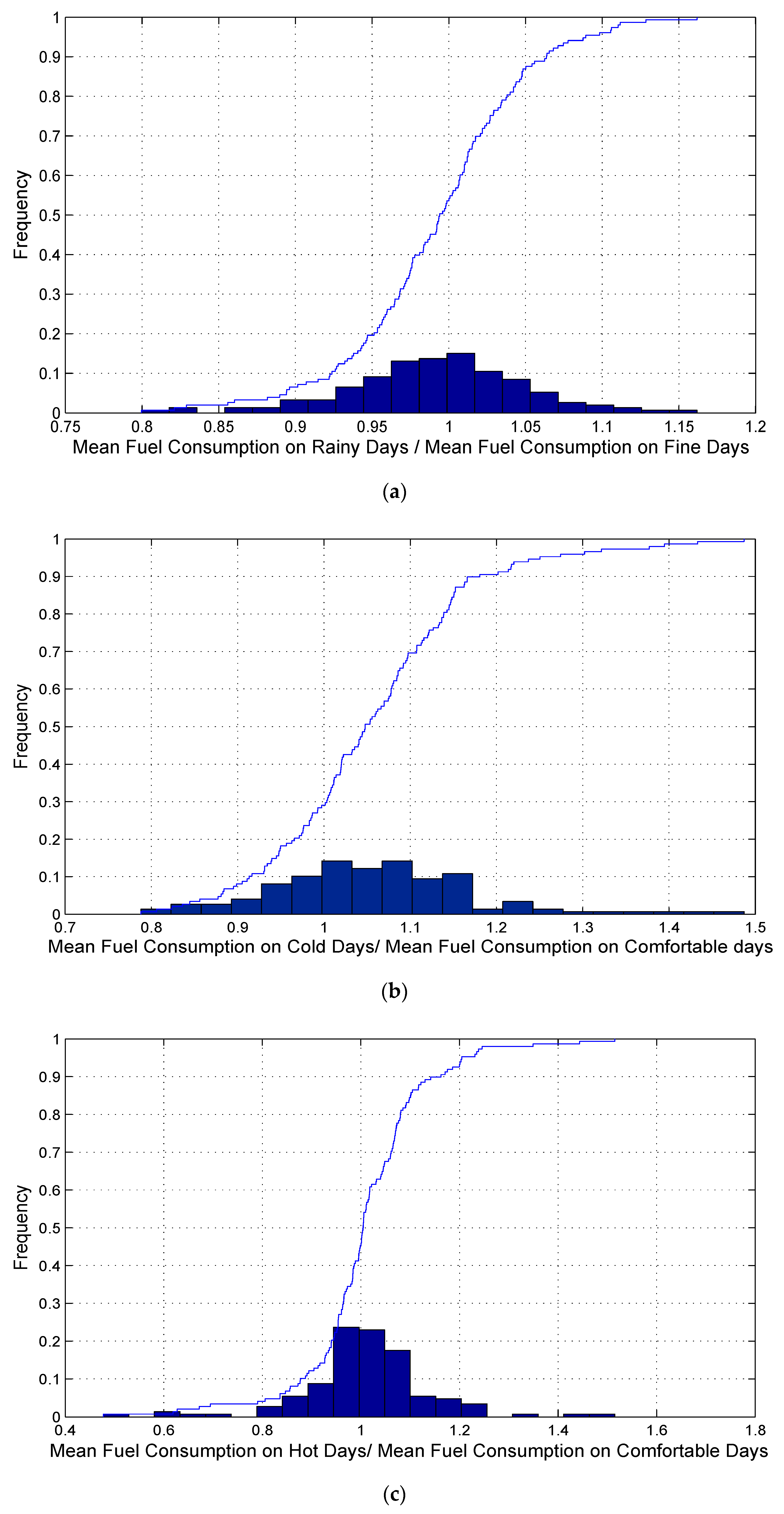
The effects of weather on drivers’ fuel efficiencies were also explored. The weather data were from the Japan Meteorological Agency, including temperature and rainfall. Figure 5a shows the distribution of the ratios of mean fuel efficiencies across rainy and fine days. Fine days refer to days without precipitation. From the t-tests, the differences of 142 drivers were significant. This indicates that it was necessary to consider these differences when modeling drivers’ daily fuel consumptions.

In this study, the days with temperatures lower than 10 °C were defined as cold days, and the days with temperatures higher than 25 °C were defined as hot days. The other days were defined as comfortable days. Figure 5b,c show the effects of cold temperature and high temperature, respectively. Based on the t-tests, 121 and 123 drivers on cold days and hot days, respectively, had fuel consumptions significantly different from those on comfortable days.

3. Incorporating Both Observed and Unobserved Multi-Level Factors

As shown in last section, the data used in this study can be categorized as hierarchical data. The observations were correlated because there was some tie to same unit: the same driver or the same date. For each driver, there were multi-observations from different days which shared some individual-specific attributes, such as drivers’ driving styles. For each day, there were multi-observations for different drivers which shared some date-specific attributes, such as the weather conditions. In addition to the individual- and date-specific attributes, there were some observation-specific attributes that affected drivers’ daily fuel consumption, such as drivers’ daily schedules.

Therefore, the factors discussed here can be divided to three parts: individual-specific, date-specific, and observation-specific. At first, we considered the following ordinary linear regression model as a solution for this problem:

$$\mathrm{Model}1:\log (\mathrm{Fue}{\mathrm{l}}_{ij})={\beta }_0+{\beta }_1{X}_i+{\beta }_2{Y}_j+{\beta }_3{Z}_{ij}+{\epsilon }_{ij},$$

(1)

where $\mathrm{Fue}{\mathrm{l}}_{ij}$ is the fuel consumption of driver i for day j; $X_i$ is the observed individual-specific attributes for driver i; $Y_j$ is the observed date-specific attributes for day j; $Z_{ij}$ is the observed observation-specific attributes for driver i on day j; ${\epsilon }_{ij}$ is the independent and identically distributed (i.i.d.) Gaussian distributed error term for each observation; ${\beta }_0$ is the constant term, while ${\beta }_{1~3}$ are parameters to be estimated.

In Model 1, $X_i$, $Y_j$, and $Z_{ij}$ represent observed heterogeneity, while ${\epsilon }_{ij}$ can be interpreted as unobserved heterogeneity. The problem of Model 1 is that it cannot consider the correlations of unobserved heterogeneity. Since drivers’ daily fuel consumption is affected by many factors and the available data are limited, it is a general situation that, in addition to attributes in $X_i$, $Y_j$ and $Z_{ij}$, there are other unobserved attributes that can significantly affects drivers’ daily fuel consumption. These unobserved attributes cause random effects crossing observations, which can also be categorized into three parts: individual-specific, date-specific, and observation-specific. In Model 1, since ${\epsilon }_{ij}$ terms are i.i.d. error terms, they can only incorporate the observation-specific unobserved heterogeneity. For the observations sharing the same driver or date, the correlations of error terms cannot be incorporated.

To incorporate unobserved individual-specific and date-specific factors, the following three multi-level models are proposed:

$$\begin{array}{l}\mathrm{Model}2:\log (\mathrm{Fue}{\mathrm{l}}_{ij})={\beta }_0+{\beta }_1{X}_i+{\beta }_2{Y}_j+{\beta }_3{Z}_{ij}+u_i+{\epsilon }_{ij}\\ \mathrm{Model}3:\log (\mathrm{Fue}{\mathrm{l}}_{ij})={\beta }_0+{\beta }_1{X}_i+{\beta }_2{Y}_j+{\beta }_3{Z}_{ij}+v_j+{\epsilon }_{ij}\\ \mathrm{Model}4:\log (\mathrm{Fue}{\mathrm{l}}_{ij})={\beta }_0+{\beta }_1{X}_i+{\beta }_2{Y}_j+{\beta }_3{Z}_{ij}+u_i+v_j+{\epsilon }_{ij}\end{array}$$

(2)

where $u_i$ and $v_j$ are Gaussian distributed random errors that represent individual- and date-specific unobserved heterogeneity, respectively.

The key points of the multi-level models were considered using the correlations of multiple observations by introducing some error terms that were shared by these observations.

Model 2 was a two-level model that considered random effects caused by both individual-specific and observation-specific factors, while Model 3 was another two-level model that considered both date-specific and observation-specific factors. Model 4, which was the combination of Model 2 and Model 3, was a three-level model that explicitly incorporated all three parts of the random effects.

It should be noted that, in Model 4, $u_i$ and $v_j$ were cross-nested, which means that, different drivers shared the same $v_j$ on the same day, while the same driver on different dates shared the same $u_i$.

4. Estimation and Analysis

All four models could be estimated by the simulated maximum-likelihood method. Because the estimation modules for multi-level models are already available in many statistical tools, such as Stata and R, the technical details of estimation are not be described in this paper.

The four models were estimated based on the whole data, data on working days, and data on holidays. The explanatory variables are described in

Table 2. Descriptions of explanatory variables.

Explanatory Variables	Description
Individual-specific
Disp	The displacement of vehicle engines; unit: L
Capacity	The capacity of vehicle; unit: tons
Hybrid	Dummy variable, 1 for hybrid vehicle
Job	Dummy variable, 1 for company employee
Age	The age in years of the driver
Gender	Dummy variable, 1 for male
Dis2Hall	The distance between home location and Toyota city hall; unit: km
Date-specific
Rain	Dummy variable, 1 for rainy day
Work_Holi	Dummy variable, 1 for holidays
Temp_0_10	Minimize(10, temperature); unit: °C
Temp_10_25	Maximize(Minimize(15, temperature–10), 0); unit: °C
Temp_25_Inf	Maximize(0, temperature–25); unit: °C
Observation-specific
Dri_Time	The total driving time for each driver on each day
Arr_Time	The arrival time of the last trip for each driver on each day
Dep_Time	The departure time of the first trip for each driver on each day

. All the driver- and vehicle-specific variables which were available in this study were considered. The dummy variable “Hybrid” was included to consider the differences between hybrid vehicles and traditional vehicles. The estimation results are shown in

Table 3. Estimation results of models for all days.

Parameters	Model 1	Model 2	Model 3	Model 4
Disp	0.547 ***	0.585 ***	0.547 ***	0.585 ***
Capacity	−0.236 ***	−0.337 ***	−0.236 ***	−0.337 ***
Hybrid	0.072 ***	−0.014	0.071 ***	−0.014
Job	0.009 **	0.018	0.009 **	0.018
Age	−0.003 ***	−0.002	−0.003 ***	−0.002
Gender	0.056 ***	0.008	0.056 ***	0.008
Dis2Hall	−0.009 ***	−0.006	−0.009 ***	−0.006
Rain	0.001 ***	0.001 ***	0.001 ***	0.001 ***
Work_Holi	−0.026 ***	−0.046 ***	−0.027 ***	−0.047 ***
Dri_Time	2.016 ***	2.765 ***	2.016 ***	2.779 ***
Arr_Time	0.070 ***	−0.068 ***	0.069 ***	−0.071 ***
Dep_Time	0.106 ***	0.080 ***	0.107 ***	0.084 ***
Temp_0_10	−0.019 ***	−0.019 ***	−0.019 ***	−0.019 ***
Temp_10_25	−0.001	−0.001	−0.001	−0.001
Temp_25_Inf	0.028 ***	0.0276 ***	0.028 ***	0.028 ***
Constant	−3.383 ***	−3.228 ***	−3.382 ***	−3.224 ***
$\mathrm{Std}({\epsilon }_{ij})$	0.160 ***	0.110 ***	0.159 ***	0.109 ***
$\mathrm{Std}(u_i)$		0.052 ***		0.052 ***
$\mathrm{Std}(v_j)$			0.000	0.001 ***
Final LL	−13,560.558	−8804.237	−13,559.432	−8794.648
N	27,044	27,044	27,044	27,044

* p < 0.05, ** p < 0.01, *** p < 0.001.

,

Table 4. Estimation results of models for working Days.

	Model 1	Model 2	Model 3	Model 4
Disp	0.546 ***	0.593 ***	0.546 ***	0.594 ***
Capacity	−0.242 ***	−0.358 ***	−0.242 ***	−0.358 ***
Hybrid	0.067 ***	−0.028	0.067 ***	−0.028
Job	0.013 ***	0.020	0.013 ***	0.020
Age	−0.003 ***	−0.002	−0.003 ***	−0.002
Gender	0.047 ***	0.002	0.047 ***	0.002
Dis2Hall	−0.011 ***	−0.006 *	−0.011 ***	−0.006 *
Rain	0.001 ***	0.001 ***	0.001 ***	0.001 ***
Dri_Time	1.555 ***	2.621 ***	1.555 ***	2.635 ***
Arr_Time	0.082 ***	−0.078 ***	0.082 ***	−0.080 ***
Dep_Time	0.100 ***	0.102 ***	0.101 ***	0.105 ***
Temp_0_10	−0.0193 ***	−0.0211 ***	−0.0193 ***	−0.0211 ***
Temp_10_25	−0.00183 *	−0.00160 **	−0.00185 *	−0.00166 *
Temp_25_Inf	0.0295 ***	0.0278 ***	0.0295 ***	0.0278 ***
Constant	−3.317 ***	−3.175 ***	−3.315 ***	−3.168 ***
$\mathrm{Std}({\epsilon }_{ij})$	0.132 ***	0.080 ***	0.132 ***	0.079 ***
$\mathrm{Std}(u_i)$		0.056 ***		0.056 ***
$\mathrm{Std}(v_j)$			0.000	0.001 ***
Final LL	−7934.506	−3328.949	−7932.938	−3315.674
N	19,460	19,460	19,460	19,460

* p < 0.05, ** p < 0.01, *** p < 0.001.

and

Table 5. Estimation results of models for holidays.

	Model 1	Model 2	Model 3	Model 4
Disp	0.536 ***	0.554 ***	0.536 ***	0.554 ***
Capacity	−0.210 ***	−0.264 ***	−0.210 ***	−0.264 ***
Hybrid	0.086 ***	0.036	0.086 ***	0.036
Job	−0.002	0.003	−0.002	0.003
Age	−0.002 ***	−0.003	−0.002 ***	−0.00303
Gender	0.0877 ***	0.0329	0.0877 ***	0.033
Dis2Hall	−0.003 ***	−0.003	−0.003 ***	−0.003
Rain	0.001 *	0.001 **	0.001 *	0.001 **
Dri_Time	2.779 ***	3.182 ***	2.779 ***	3.182 ***
Arr_Time	0.010	−0.075 *	0.010	−0.075 *
Dep_Time	0.174 ***	0.123 **	0.174 ***	0.124 **
Temp_0_10	−0.017 ***	−0.016 ***	−0.017 ***	−0.016 ***
Temp_10_25	0.002	0.002	0.002	0.002
Temp_25_Inf	0.024 ***	0.025 ***	0.024 ***	0.025 ***
Constant	−3.573 ***	−3.396 ***	−3.573 ***	−3.396 ***
$\mathrm{Std}({\epsilon }_{ij})$	0.225 ***	0.176 ***	0.225 ***	0.176 ***
$\mathrm{Std}(u_i)$		0.050 ***		0.050 ***
$\mathrm{Std}(v_j)$			0.000	0.000
Final LL	−5108.663	−4379.890	−5108.663	−4379.818
N	7584	7584	7584	7584

* p < 0.05, ** p < 0.01, *** p < 0.001.

. In Table 3, all the models were estimated with observations on all days. To consider the differences between holidays and working days, a dummy variable “Work_Holi” was incorporated. Since the observations were abundant enough, we also estimated the models with observations on working days and holidays. The estimation results are shown in Table 4 and Table 5, respectively.

At first, according to the likelihood-ratio test based on the finallog-likelihoods (LLs) shown in Table 3, Table 4 and Table 5, it can be found that, for all models, it was better to estimate parameters for holidays and working days separately. The parameters of Work_Holi in Table 3 were all negative and significant at the 0.001 level, which indicates that fuel consumption on holidays was significantly less than that on working days. This finding is reasonable. The possible explanation is that, on working days, most trips are commuting trips, which are made in peak hours, while trips on holidays are more dispersive. The possible congestion in peak hours will cause higher fuel consumption on working days.

Then, our attentions turned to the final LLs in Table 4 and Table 5. In this study, to consider the multi-level random effects, three error terms were incorporated in Model 4. According to the likelihood-ratio tests based on the final LLs, the model fit on working days was significantly enhanced by incorporating all three error terms, compared with all other models. However, on holidays, Model 4 did not significantly fit the data better than Model 2, which did not consider the date-specific unobserved factors. These findings indicate that, for working days, it was necessary to consider all three levels of unobserved factors, which could not be well described by the observed explanatory variables, while, on holidays, the date-specific factor was already well described by the observed date-specific explanatory variables; thus, it was not necessary to incorporate the date-specific error term. The final LLs of Model 2 for both working days and holidays were significantly higher than those of Model 1. This indicates that the individual-specific explanatory variables in this study could not well described drivers’ individual-specific characteristics that affect their fuel consumption; therefore, an individual-specific error term had to be incorporated.

The findings above could also be confirmed with the p-values of estimated parameters. With Model 4, the estimates of $\mathrm{Std}(v_j)$ were significantly different from 0 on both working days and holidays, while $\mathrm{Std}(v_j)$ was not significant on holidays. Comparing results of Model 1 and 2, it was interesting to find that, in Model 1, the estimates of all parameters were significant; however, when the unobserved individual-specific error term was incorporated, the estimates of parameters on some individual-specific explanatory variables became not significant. Since p-values are an important basis of behavior analysis, this implies that, if the multi-level random effects are not explicitly incorporated, in addition to a decrease in model performance, it is also possible to get some wrong behavioral findings.

At last, we analyzed the estimates of parameters. Since Model 4 had the best model fit, our findings were based the estimation results of Model 4. Considering the individual-specific characteristics, according to the signs of parameters Disp and Capacity, it can be found that drivers with higher-displacement and low-capacity vehicles consumed more fuel per unit driving distance. Considering the date-specific characteristics, the positive sign of the Rain parameter indicates that fuel consumption on rainy days was higher than that on fine days. The shape of the piecewise definition of temperature with estimated parameters indicates that, on cold days, fuel consumption increased with the decrease in temperature, while, on hot days, fuel consumption increased with the increase in temperature. A possible explanation is the usage of air conditioners on hot days and cold days. Regarding the observation-specific characteristics, it can be found that, when drivers departed home later and arrived home earlier, driving for a longer time, their fuel consumption was higher, according to the signs of parameters Dep_Time, Arr_Time, and Dri_Time.

5. Conclusions

This study explored drivers’ daily fuel consumption efficiency and related factors, based on the long-term CAN (Controller Area Network) data collected by private vehicles in Toyota, Japan. The daily fuel consumption was defined as the daily average fuel consumption for a unit of driving mileage, expressed in liter per hundred kilometers (L/100 km), an index measure of drivers’ fuel efficiencies. Based on the descriptive statistics and statistical tests, multi-level heterogeneities were preliminarily proven to be significant.

Then, models were proposed to consider the multi-level random effects simultaneously: individual-specific, date-specific, and observation-specific. To explore these multi-level observed heterogeneities, explanatory variables which described drivers’ characteristics, attributes of each date, and characteristics related to specific observations were incorporated in developed models. In addition to the observed factors, there were still some factors that could not be described by the explanatory variables, which would cause random effects. The random effects were incorporated by the multi-level specifications of error terms in the developed models.

Four models with different specifications of error terms were estimated based on the hierarchical panel data and compared with each other. From the estimation results, we found it necessary to develop models for holidays and working days separately. Fuel consumption on holidays was significantly lower than that on working days.

It was also found that it was not always necessary to consider all three levels of random effects. In this study, on working days, model fit was significantly enhanced by incorporating all three error terms, compared with all other models, while the date-specific random effects were found to be not significant.

Several behavioral findings were also obtained based on the estimation results. Drivers with higher-displacement and low-capacity vehicles consumed more fuel per unit driving distance. Fuel consumption on rainy days was higher than that on fine days. On cold days, fuel consumption increased with the decrease in temperature, while fuel consumption increased with the increase in temperature on hot days. When drivers departed home later and arrived home earlier, driving for a longer time, their fuel consumption was higher.

In this study, drivers’ driving behavior was not considered. In future research, we can analyze drivers’ driving patterns using the CAN data and combine it with fuel consumption analysis. Fuel consumption is only one measure of drivers’ car usage. In the future, we can develop models with multi-outputs to consider the correlations between different car usage measures, such as travel time and mileage.

References

- El-Shawarby, I.; Ahn, K.; Rakha, H. Comparative field evaluation of vehicle cruise speed and acceleration level impacts on hot stabilized emissions. Transp. Res. Part D Transp. Environ. 2005, 10, 13–30. [Google Scholar] [CrossRef]
- Zhang, K.; Frey, H.C. Road grade estimation for on-road vehicle emissions modeling using light detection and ranging data. J. Air Waste Manag. Assoc. 2006, 56, 777–788. [Google Scholar] [CrossRef] [PubMed]
- Chen, C.; Huang, C.; Jing, Q.; Wang, H.; Pan, H.; Li, L.; Zhao, J.; Dai, Y.; Huang, H.; Schipper, L.; et al. On-road emission characteristics of heavy-duty diesel vehicles in Shanghai. Atmos. Environ. 2007, 41, 5334–5344. [Google Scholar] [CrossRef]
- Ross, M. Automobile fuel consumption and emissions: Effects of vehicle and driving characteristics. Annu. Rev. Energy Environ. 1994, 19, 75–112. [Google Scholar] [CrossRef]
- Tang, T.-Q.; Yi, Z.-Y.; Lin, Q.-F. Effects of signal light on the fuel consumption and emissions under car-following model. Phys. A Stat. Mech. Appl. 2017, 469, 200–205. [Google Scholar] [CrossRef]
- Koffler, C.; Rohde-Brandenburger, K. On the calculation of fuel savings through lightweight design in automotive life cycle assessments. Int. J. Life Cycle Assess. 2009, 15, 128. [Google Scholar] [CrossRef]
- Delogu, M.; del Pero, F.; Pierini, M. Lightweight Design Solutions in the Automotive Field: Environmental Modelling Based on Fuel Reduction Value Applied to Diesel Turbocharged Vehicles. Sustainability 2016, 8, 1167. [Google Scholar] [CrossRef]
- Del Pero, F.; Delogu, M.; Pierini, M. The effect of lightweighting in automotive LCA perspective: Estimation of mass-induced fuel consumption reduction for gasoline turbocharged vehicles. J. Clean. Prod. 2017, 154, 566–577. [Google Scholar] [CrossRef]
- Axhausen, K.W.; Gärling, T. Activity-based approaches to travel analysis: Conceptual frameworks, models, and research problems. Transp. Rev. 1992, 12, 323–341. [Google Scholar] [CrossRef]
- Hatzopoulou, M.; Hao, J.Y.; Miller, E.J. Simulating the impacts of household travel on greenhouse gas emissions, urban air quality, and population exposure. Transportation 2011, 38, 871–887. [Google Scholar] [CrossRef]
- Snijders, T.A.; Bosker, R.J. Multilevel Analysis: An Introduction to Basic and Advanced Multilevel Modeling; SAGE: Newcastle upon Tyne, UK, 2011. [Google Scholar]
- Casaló, L.V.; Escario, J.-J. Heterogeneity in the association between environmental attitudes and pro-environmental behavior: A multilevel regression approach. J. Clean. Prod. 2018, 175, 155–163. [Google Scholar] [CrossRef]
- Ritz, C.; Laursen, R.P.; Damsgaard, C.T. Simultaneous inference for multilevel linear mixed models—With an application to a large-scale school meal study. J. R. Stat. Soc. Ser. C (Appl. Stat.) 2017, 66, 295–311. [Google Scholar] [CrossRef]
- Ding, C.; Lin, Y.; Liu, C. Exploring the influence of built environment on tour-based commuter mode choice: A cross-classified multilevel modeling approach. Transp. Res. Part D Transp. Environ. 2014, 32, 230–238. [Google Scholar] [CrossRef]
- Hess, S.; Train, K.E. Recovery of inter- and intra-personal heterogeneity using mixed logit models. Transp. Res. Part B Methodol. 2011, 45, 973–990. [Google Scholar] [CrossRef]
- Hess, S.; Rose, J.M. Allowing for intra-respondent variations in coefficients estimated on repeated choice data. Transp. Res. Part B Methodol. 2009, 43, 708–719. [Google Scholar] [CrossRef] [Green Version]
- Park, Y.; Akar, G. Why do bicyclists take detours? A multilevel regression model using smartphone GPS data. J. Transp. Geogr. 2019, 74, 191–200. [Google Scholar] [CrossRef]
Figure 1.
The study network and distributions of trip destinations.
Figure 2.
The distributions of average fuel consumption. (a) Frequency histograms and cumulative curves of daily average fuel consumption, i.e., average values across drivers on each date. (b) Frequency histograms and cumulative curves of drivers’ personal average fuel consumption, i.e., average values across days for each driver.
Figure 3.
The variations of fuel consumption: frequency histograms and cumulative curves of coefficients of variation (CVs). (a) Inter-individual variation: distributions of CVs calculated across drivers. (b) Time variation: distributions of CVs calculated across days.
Figure 4.
Frequency histograms and cumulative curves of ratios of fuel efficiencies on holidays and working days.
Figure 5.
The effects of weather on fuel consumption. (a) The effects of rain: frequency histograms and cumulative curves of ratios of mean fuel efficiencies across rainy and fine days. (b) The effects of low temperature: frequency histograms and cumulative curves of ratios of mean fuel efficiencies across cold and comfortable days. (c) The effects of high temperature: frequency histograms and cumulative curves of ratios of mean fuel efficiencies across hot and comfortable days.