County-Scale Destination Migration Attractivity Measurement and Determinants Analysis: A Case Study of Guangdong Province, China


1
School of Geography & Tourism, Guangdong University of Finance & Economics, Guangzhou 510320, China
2
Department of Management, Guangdong Polytechnic Normal University, Guangzhou 510665, China
3
Population Studies and Training Center, Brown University, Providence, RI 02912, USA
*
Author to whom correspondence should be addressed.
Sustainability 2019, 11(2), 362; https://doi.org/10.3390/su11020362
Submission received: 30 November 2018
/
Revised: 28 December 2018
/
Accepted: 9 January 2019
/
Published: 12 January 2019
(This article belongs to the Section Sustainability in Geographic Science)
Abstract
:Measuring destination attractivity and finding the determinants of attractivity at the county scale can finely reveal migration flows and explain what kinds of counties have higher attractivity. Such understanding can help local governors make better policies to enhance county attractivity and attract more migrants for regional development. In this study, the county-scale relative intrinsic attractivity (RIA) of Guangdong Province is computed using the number of migrants and the corresponding distances between origins and destinations. The results show that the RIA has a higher positive correlation with the flows of migrants to destination and demonstrates an obvious phenomenon of distance decay. The RIA decreases faster when the distance between origins and destinations increases. Spatially, the RIA reveals a core-periphery belt pattern in Guangdong Province. The center of the Pearl River Delta is the highest core of RIA and the outside areas of the delta represent the low-RIA belt. The highest RIA is 6811 in Dongguan City and the lowest RIA is 1 in Yangshan County. The core area includes Dongguan, Shenzhen City and the southern regions of Guangzhou, Foshan and Zhongshan City where the RIA value is higher than 1000. The second belt is mainly composed of the periphery districts of the Pearl River Delta, which include Shunde, Nanhai, Luohu, Tianhe Huicheng, Panyu, Haizhu, Huiyang, Huadu, Yuexiu, Xiangzhou and the Yuexiu, Huangpu and Boluo, where the RIA values are higher than 100 and lower than 1000. The third belt includes the western wing, eastern wing and northern area. Most of these RIA values range from 1 to 2. In this belt, there are three areas with relatively higher RIA attractivity scattered in the ring: the downtowns of Zhanjiang City, Chaozhou and Shantou Cities and Shaoguan City. The areas farther away from the core have a lower RIA score. Determinants analysis indicates that the RIA is positively determined by destination economic development level, social service and living standard level and destination population quality. A region will be more attractive if it has higher per capital GDP, tertiary industry level, investment and number of industrial enterprises involved in economic development. A region with a high annual average wage of employees and high social service and living standards will be more attractive, while a region with low destination population quality, including aspects such as the adult illiteracy rate, will be less attractive.
1. Introduction
Migration from less developed and rural regions to developing and urban regions has become an intrinsic process of regional economic development [1,2,3,4,5,6]. With the rapid world economic development, the stock of international migrants reached to 258 million and the proportion of international migration in the world population is 3.4% in 2017 [7]. Asia, Europe and North American are the main destinations of migrants and the in migrants of them were 80 million, 78 million and 58 million respectively while Asia, Europe, Latin American and Africa are the main migration origins and the out migrants were 110 million, 64 million, 39 million and 38 million respectively in 2017 [7]. Asia is the first place international migration destination and origin in the world. In Asia, China has the largest population size in the world and the migration flow of China is one of the most important flows of world migration.
The Chinese economy has developed rapidly in the 40 years since the beginning of China’s Reform and Opening policy. The real GDP per capita increased from 381 Yuan in 1978 to 59,262 Yuan in 2017 and the real GDP per capita in 2017 was 150 times that in 1978. Migration has increased in step with the rapid economic development, industry development and urbanization in China [8]. The number of migrants from less developed areas to developed areas in China increased from 39.6 million to 121.0 million during the period 1990 to 2000 [9,10] and further increased to 247 million at the end of 2015 [11]. The internal migration of China is considered the largest migration in the world [12].
Because of the rapid economic development in China, this large-scale internal migration has become a research hotspot internationally. Studies have mainly focused on four aspects of migration. The first was the impacts of migration on the destination economy, society and environment. For example, Fan studied the migration flows among provinces and impacts on destination economic development in China from 1990 to 2000 [13]. In early 1994, Wu studied the hukou system and migration in China [14]. Chan et al. later studied the hukou registration system and depicted migrant flows from rural to urban areas over space and time [15,16], especially focusing on rural migrant labor and the contributions to the development of manufacturing at the migration destinations [15]. They think that the hukou system enables China to create a massive exploitable migrant labor force that makes China’s industry highly competitive in the global economy. With the deepening of the Reform and Opening policy in China, a ‘new normal’ pattern of economic development is sought that will involve sustainable development with slower economic growth and better growth quality, social equality and environmental protection. Based on the new development pattern, Shen and Xu studied migration patterns and impacts on the regional economy, society and environment of both destinations and origins [8]. The current migration pattern has led to significant changes in regional economic structure that have accelerated urban development and weakened the development of rural areas. The second focus was migration flows and the characteristics of different migrant groups [13,17,18,19]. Scholars thought that the migration flows were mainly from rural to urban areas and that interprovincial flows were mainly from less developed areas to developed eastern coastal provinces. The two main kinds of flows increased gradually along with the educational level of migrants from 2000 to 2010 [20,21,22]. The third focus was mainly the determinants and mechanism of migration [9,23,24,25]. Most studies showed that the imbalanced economic situation among origins and destinations was the main factor driving migrants to leave their origins for abundant job opportunities in urban destinations. The fourth focus was the reform of China’s hukou registration system and medical insurance system, which also increased migration in China [26,27].
Since 2017, China has stepped into a ‘new era’ in which labor and talent are the most valuable resources for regional development. Most cities are trying to attract more laborers and talents. The power of cities or districts (counties) to draw laborers and talent from other areas is very important to regional development; therefore, enhancing destination attractivity is an important task for local governments. However, few scholars have studied destination attractivity, while current studies of migration are mainly focused on the characteristics of migrants, interprovincial migrant flows and impacts on the economy, society and environment of migration destinations in China. Most scholars have used numbers or rates of in-migration or net migration as the main indices of migration flows [11,15,18,19,28,29,30,31]. However, Fotheringham et al. indicated that the most commonly used indices, such as the numbers and rates of in-migration and net migration, have some deficiencies in accurately assessing destination attractiveness [32], as such measurement methods ignore the geography of the situation. If destination attractivity is determined according to inflows, a higher attractivity might be found simply if the destination is located very close to heavily populated migration origins even if the destination may have few attractive characteristics. The attributes of the destination may have very little influence on the migration inflows if migrants’ moving decisions are affected mainly by the closer geographical distance between origin and destination. In the same way, a destination might have a relatively low inflow simply because it is relatively inaccessible to migrants from most origins, even if it has many attractive characteristics [32]. Thus, destination attractivity research is now important for policy making and regional development in China. Moreover, few studies have been carried out to find the migration patterns at the county scale [33]. In China, most provinces are vast and there are obvious differences inside provinces. Based on intra-provincial differences and the characteristics of the new era, district-(county-)scale attractivity for migrants should be given more attention to reveal migration flows in detail and show what types of county have higher attractiveness. Currently, there are some policies for attracting migrants at large scale regions such as Pearl River Delta, Yangtze River Delta in China. However, there are scare policies to attract migrants at county scale that hinder migrants move into such small spatial unit for regional development. The knowledge that enhances county-scale destination migration attractivity will help local governors make better policies to enhance county attractivity and attract more migrants for regional development.
In this paper, we hope to fill in the gap of measuring county-scale migration attractivity and finding out whether the county-scale RIA of China differences spatially. Therefore, we hope to answer the following questions: how can we measure county-scale RIA and how can we analyze RIA spatial differences? What county determinants affect RIA and how? To answer these questions, this paper first introduces the study area, Guangdong Province and the data sources and methods concerned with destination attractivity measurement, spatial distribution and determinants analysis. The third section presents the main results of the destination attractivity and RIA determinants. The fourth section concludes and discusses destination attractivity and the determinant of migration.
2. Study Area, Materials and Methods
2.1. Study Area
We choose Guangdong Province as the study area for county-scale attractivity measurement and determinants analysis. Guangdong Province is located in southern China (Figure 1) and consists of 21 cities, including Guangzhou, Shenzhen, Zhuhai and Shantou. Shenzhen, Zhuhai and Shantou represented the first group of special economic zones that led to rapid regional economic development. Based on the difference in topography and the level of economic development, Guangdong Province is usually divided into four regions: the Pearl River Delta, the western wing region, the eastern wing region and the northern region.
Since 1988, the total GDP of Guangdong Province has held first place among that of all provinces, municipalities and autonomous regions of China, reaching 4195 trillion Yuan at the end of 2017. However, the imbalanced economic situation within the province of Guangdong is one of the main problems in the development process. In 2017, the GDP of the Pearl River Delta represented 79.7% of the GDP of the entire province, while the GDP of the eastern wing, northern area and western wing was 6.8%, 6.0% and 7.5%, respectively. With the rapid economic development, many migrants moved to Guangdong Province from less developed areas in China. Migrants to Guangdong Province represented 13% of all migrants in China in 2015, reaching 32 million in number at the end of 2015. Most migrants, amounting to 29 million in 2015, clustered in the Pearl River Delta areas. Since the migration to Guangdong Province is typical of migration in China, Guangdong is a suitable choice for a case study.
2.2. Materials
2.2.1. Migration Data
Migration volume, the most important index for measuring destination RIA, is defined as the number of migrants who changed residence between two specific areas over a period of time. Someone is considered a migrant if ‘the current place (county scale) of residence on the date of enumeration was different from their permanent residence 5 years ago’ and the current place of residence is considered the usual residence of the migrants if they have been away from their former place of household registration for more than one year. The migration data used in this research are derived from the 2010 Guangdong Population Census, which covers the volume of the county-level in-migration of 123 districts in Guangdong province and migrants’ origin province and destination district (county). Though there are migration flows among counties of Guangdong Province, we do not consider intra-provincial migration in this research because the origin-destination intra-provincial migration flow cannot be obtained from the current population census.
2.2.2. Migration Distance
When measuring destination attractivity, migration distance is another important variable. In this study, we compute the road distance from migrants’ origin to the destination at the county scale. Migrants’ origins are defined as the capital city of the province, while county-scale destinations are defined as the center of the county in which the migrants currently residence. For example, the hometown of a migrant is in Ledu County, a county of Qinghai Province and he moves into Panyu District, a district (county) of Guangdong Province. The origin location will be defined as the center of Xining City, the capital of Qinghai Province and the destination location will be defined as the center of Panyu district, Guangdong Province. The road distances are automatically calculated in the Gaode map system.
2.2.3. Migration Determinants
Many studies have investigated migration determinants [34,35,36,37,38,39,40,41,42,43]. For example, Fan’s research indicated that the interprovincial migration flow in China has a strong relationship with regional development, as many migrants moved from relatively poor central and western provinces into rapidly growing economic regions in the early 1990s [13]. Li’s research indicated that place attractiveness seems to be determined mainly by demographic and socioeconomic factors, while physical factors have a very small influence [44]. Delisle and Shearmur thought that the talent migration flows of Canada are strongly dependent on basic gravity variables, such as size and distance but that other variables (such as income differences, presence of graduates and border effects) do not affect all flows equally and wage levels in fact operate only at a provincial level [45]. Niedomysl and Hansen’s research indicated that in the decision to move, jobs are considerably more important than certain amenities among highly educated migrants compared with migrants with lower education [46]. Liu and Shen’s research indicated that employment opportunities, especially interregional wage differentials, play a dominant role in attracting skilled labor, while the impact of amenities on skilled migration turns out to be small and less clear [19]. Gries thought that average wages, unemployment rates, urbanization and income disparity are pull factors and rural poverty and average wage are push factors of migration in China [47]. Shen and Liu also found that less-skilled migrants tended to leave areas with a large population, small non-agricultural sector, high unemployment rate and small amount of foreign investment [31]. Fan’s research indicated that interprovincial migration is positively correlated with the level of economic development in the migration origin and the population scale in the origin and destination [36]. Based on current determinants analysis, destination economic development level, employment opportunities and average wage are the main determinants of migration; therefore, destination economic development, social service and living standards and destination population quality are chosen as the determinants for destination attractivity. The corresponding variables are shown in Table 1.
There are14 total determinants in the whole model; 8 determinants of economic dimension, 3 determinants of social service and living standard dimension and 3 determinants of destination population quality level dimension.
2.3. Methods
2.3.1. Destination Attractivity Measurement
Since traditional migration indices have deficiencies in accurately assessing destination attractiveness for ignoring the geography of the situation and distance between origins and destinations, more accuracy method such as relative intrinsic attractivity (RIA) can be used to solve the problem with combining migrant numbers and moved distance. Attractivity is usually called relative intrinsic attractivity (RIA) and it is a relative concept. Therefore, there are no units for attractivity in absolute terms. RIA is usually used to show the difference between two places; for example, place A may be two times more attractive than place B [32]. Suppose variable Mij is the migration flow from origin i to destination j and variable dij is the migrant’s moved distance from origin i to destination j. An equation of migration flow and distance is formulated as follows:
where Dj is a dummy variable that takes 1 when the migration flow is to destination j and 0 otherwise. The RIA values of the destinations are then computed using the parameters of a in this model. The complete derivation process can be found in Fotheringham’s research [32]. When estimating the parameters of a, one destination must be removed from Equation (1). The RIA value for the destination removed from Equation (1) is computed by:
and the RIA for the other destinations are given by:
RIA (removed_destination) = exp(a0)
RIA (included_destination j) = exp(a0 + aj)
Then, it is generally rescaled as:
RIA (rescaled) = RIA/minimum (RIA)
2.3.2. Attractivity Spatial Difference Measurement—Global Spatial Autocorrelation
The indices of spatial association analysis can reveal the clusters of a feature in space. Compared with the commonly used hierarchical thematic map, spatial autocorrelation can find both the high-high or low-low clusters and the low-high or high-low clusters. The global spatial autocorrelation can reveal the spatially cluster pattern in the whole region while the local spatial autocorrelation can reveal the spatially cluster pattern in the local unit. We can find the high-high or low-low or high-low or low-high different cluster patterns of migration with spatial autocorrelation and the cluster information is richer than hierarchical thematic map. The spatial autocorrelation index measures spatial autocorrelation using the values and locations of features simultaneously. The global Moran’s I index is computed as follows [48]:
where n is the number of features, zi is the deviation of feature i (), wi,j is the spatial weight of features i and j and S0 is the sum of all spatial weights:
The value range of the global Moran’s I falls between −1 and 1. The larger the absolute value, the more spatially clustered the feature attribute is.
Accompanied with global Moran I index, a z-score and corresponding p-value will be computed to explain whether the feature’s spatial cluster is statistically significant or not. The ZI for the statistic is computed as:
where,
The spatial distribution of a feature is considered random if the p-value is not statistically significant. Otherwise, the spatial distribution is more spatially clustered if the z-score is positive while it is more spatially dispersed if the z-score is negative.
2.3.3. Attractivity Spatial Difference Measurement Method—Local Spatial Autocorrelation (LISA)
Spatial clustering of migrants at a local level can be tested using local spatial autocorrelation [49]. The cluster in individual units can be studied using Local Moran’s I (Ii) for each spatial unit. It can be computed as follows:
where Zi is the deviation of the attribute of feature i from the mean, the summation over j is that only neighbors’ value of j is included and wij is a spatial weight that is equivalent to 1 if feature i is a neighbor of feature j and 0 otherwise. The value of m2 can then be computed by:
where N is the number of features. The value of local Moran I falls between −1 to 1. A positive value of local Moran I with significance p-value for feature i indicates that the feature is surrounded by features with similar values. This is associated with high-high or low-low spatial patterns. A negative value of local Moran I with significance p-value for feature i show that the feature is surrounded by features with dissimilar values. This will associate with high-low or low-high spatial distribution pattern.
2.3.4. Determinants Analysis
In general, determinants analysis is tested using a regression model after possible determinants are chosen as follows [32,50]:
where y is the RIA of a county, k is an intercept to be estimated and xi represents the independent variables. Parameter ai represents the elasticity of the relationship between RIA and the corresponding independent variable. This equation was chosen for the relationship among RIA and the independent variables because a preliminary investigation suggested that several of the relationships are non-linear [32]. This form of model also produces elasticity that is independent of the units of data measurement. The model is usually calibrated by ordinary least-squares regression after first taking natural logarithms of both sides of the equation, as follows:
One of the problems in the current regression model after taking the natural logarithms of both sides is that the independent variables should have no correlation with each other, while many economic variables and social service variables are correlated; these shortcomings of determinants analysis must be overcome in the regression model. Ridge regression is a good way to solve the problem [51,52,53,54,55,56,57]. Ridge regression is a technique for analyzing multiple regression data that suffer from multicollinearity. When multicollinearity occurs, least squares estimates are unbiased but their variances are large and may be far from the true value. By adding a degree of bias to the regression estimates, ridge regression reduces the standard errors and the net effect is expected to provide more reliable estimates. Compared with another biased regression technique, principal components regression, ridge regression is more popular [58].
Suppose that the regression equation is written in matrix form as follows:
where E(Ɛ) = 0, E(Ɛ’Ɛ) = σ2I and X is (N x p) and full rank. To facilitate comparisons among models, variables are standardized so that the matrix (X′X) is in the form of a correlation matrix and the vector (X′Y) is the vector of correlation coefficients between the criterion variable and all the independent variables.
In ordinary least squares, the regression coefficients are estimated using the following formula:
The parameters obtained are unbiased; that is, E() = β. Since X′X is the correlation matrix of independent variables, these estimates are unbiased so that the expected values of the estimate are the population values. Ridge regression proceeds by adding a small value, k, to the diagonal elements of the correlation matrix, as follows:
where k is a dimensionless scalar and . This estimate is biased. It can be shown that there exists a value of k for which the mean squared error (the variance plus the bias squared) of the ridge estimator is less than that of the least squares estimator. The objective of this procedure is to take a small bias in parameter estimation and substantially improve the mean squares of the estimates and prediction. One of the main obstacles in using ridge regression is choosing an appropriate value of k. Hoerl and Kennard suggested determining k by using a graph called the ridge trace [51]. When viewing the ridge trace, one picks a value for k for which the regression coefficients have stabilized. Often, the regression coefficients will vary widely for small values of k and then stabilize. When the smallest possible value of k is chosen (which introduces the smallest bias), the regression coefficients seem to remain constant.
In our study, ridge regression is used to find the relative importance of determinants when the independent variables are correlated and multicollinearity occurs in the regression model.
3. Results
3.1. RIA Measurement
After migration flow data Mij and migrants’ moved distance data dij are obtained, the parameter values of ai can be computed by calibrating Equation (1). When the value of ai is estimated, one destination must be removed from the equation. Fotheringham proved that this does not affect the value of RIA regardless of which destination is removed [32]. In our research, we remove Liwan District in Guangzhou City. Then, an adjusted R-squared value of 0.53 is computed with the distance-decay parameter value of −1.74 and a standard error of 4.50 from Equation (1). It also produces estimates for each of the 123 destination-specific constant terms. Then, the RIA values for each district are shown in Figure 2. The top 30 districts (counties) of the RIA are listed in Table 2. Figure 3 is a scatterplot of the RIA scores with the in-migrant volume (Figure 3).
Figure 3 indicates that there are higher similarities between RIA scores and in-migrants and the determinant coefficient associated with RIA scores and the in-migrants variable is 0.98.
3.2. RIA Spatial Difference
The global spatial autocorrelation measurement index Moran’s I is computed to find RIA global distribution states using GeoDa software. When computing the global Moran’s I index, the neighborhood of feature weight is defined as a rook contiguity neighbor, which means that two features are neighbors if they share one common boundary. The value of the Moran’s I index is 0.41, with a p-value of 0.001. The ZI score is 8.52. Based on the global spatial autocorrelation analysis, the p-value is statistically significant and the z-score is positive, which means that the spatial distribution of RIA is more spatially clustered. The Moran’s I value is positive, which means that the high-value RIA features cluster together and the low-value RIA features cluster together.
Figure 4 shows the global RIA spatial difference. The RIA of Guangdong Province forms the spatial structural pattern of a core-periphery belt. The core of the pattern is the areas of highest attractivity, which are mainly found in the center of the Pearl River Delta. This area includes Dongguan, Shenzhen City and the southern regions of Guangzhou, Foshan and Zhongshan City. The RIA value is higher than 1000 and the highest RIA value (6811) appears at Dongguan. The Baoan district has the second highest RIA value, 5400. In this core area, the RIA values of Baiyun District, Zhongshan City, Futian District and Nanhai District fall from 1000 to 1452. The second belt is mainly composed of the periphery districts of the Pearl River Delta, which include Shunde, Nanhai, Luohu, Tianhe Huicheng, Panyu, Haizhu, Huiyang, Huadu, Yuexiu, Xiangzhou and the Yuexiu, Huangpu and Boluo. The RIA values in the belt are higher than 100 and lower than 1000, representing the second most attractive area in Guangdong Province. The third belt includes the western wing, eastern wing and northern area. Most of these RIA values fall from 1 to 2, indicating that this is the area with the lowest attractivity in Guangdong Province. In this belt, there are three areas with relatively higher RIA attractivity scattered in the ring: the downtowns of Zhanjiang City, Chaozhou and Shantou Cities and Shaoguan City.
Furthermore, the LISA values are computed with GeoDa software to find the significance clustered areas. The results are shown in Figure 4.
Figure 4 shows that one high-high RIA clustered area emerges which is located in the eastern area of the Pearl River Delta. Dongguan City, Shenzhen City and Foshan City are the main regions of the highest RIA spatially clustered area, which means that the RIA values of these districts and their neighbors are all high. There emerges a low-high RIA clustered area that includes the eastern area of Guangzhou City and the western area of Huizhou city. A large low-low RIA ring appears from the western area to the eastern area across the northern area, which includes most districts and counties of Maoming, Yangjiang, Yunfu, Zhaoqing, Qingyuan, Shaoguan and Meizhou cities. Two rings emerge where the RIA values appear as random patterns. The first randomly distributed ring is located between the center of the Pearl River Delta and its periphery areas. In this ring, some districts have high RIA values, while other districts have low RIA values, which means that some districts developed first and attracted more migrants than others. The second randomly distributed ring appears mainly at the west, north and east periphery of Guangdong Province. The downtown areas of the cities in this ring are developed first and attracted many migrants, while other counties attracted few migrants.
3.3. Determinants Analysis
For finding the possible determinants of RIA, traditional ordinary least-squares (OLS) regression model is run to test the multicollinearity of independent variables. The results show that the variance inflation factor (VIF) of variables x1, x2, x3 and x6 is higher than 10 and the highest VIF is 33.53 with x1 meaning that there is significant multicollinearity of independent variables; as such, traditional regression model may not the best one for identifying determinants. The possible determinants of RIA scores are then identified based on ridge regression analysis with SPSS software since the ridge regression model can overcome the multicollinearity.
The first step is to take the natural logarithms of both RIA and the possible determinants. The second step in ridge regression analysis is to standardize the variables (both dependent variable and independent variables) as follows:
where xi represents the variables, is the mean of variable x and σ is the standard deviation of variable x. After running the ridge regression program with standardized variables in SPSS, the third important step is to choose an appropriate value of k. In our study, the ridge trace graph (Figure 5) is used to choose the value of k that Hoerl and Kennard suggested [51]. When the value of k equals 0.25, the regression coefficients become stable; therefore, we choose 0.25 as the value of k. When k equals 0.25, the regression coefficients and significance are shown in Table 3, in which the independent variables x6, x8, x11, x12 and x14 are not statistically significant at the 95% level. Then, the ridge regression program is run again with statistically significant independent variables and the value of k is chosen to 0.25. The final model results are shown in Table 4, in which all independent variables are statistically significant at the 95% level. The adjusted r-squared associated with the regression model is 0.80 and the model is therefore acceptable.
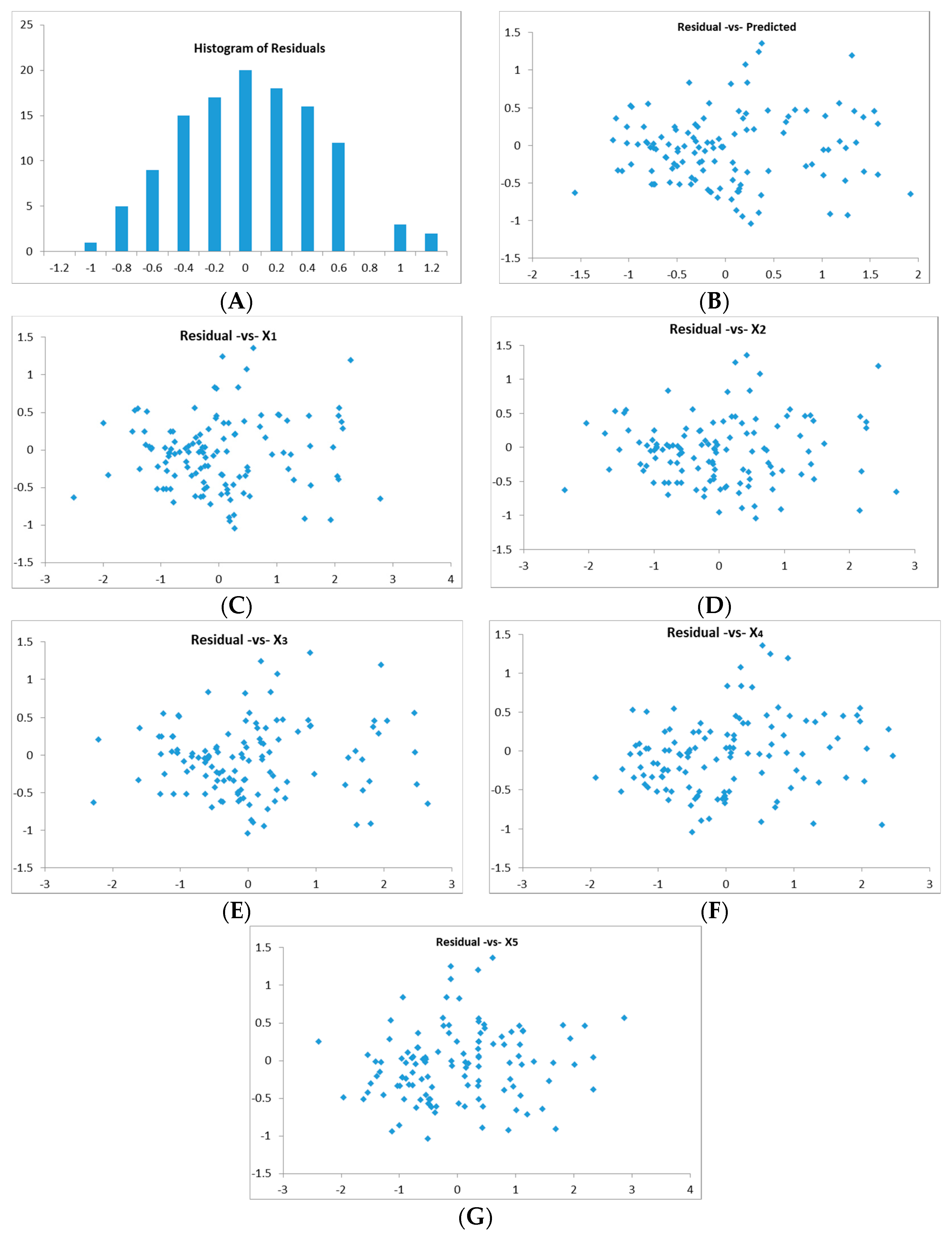
Furthermore, the ridge regression model was validated with residual analysis to test the assumption of normality, homoscedasticity of error and statistical independence. The normal probability plot of error shows that the error distribution is normal (Figure 6A). Residual versus predicted value plot and residual versus independent variable plots are created to test homoscedasticity of error and statistical independence (Figure 6B–G). The errors do not systematically get larger or become smaller in one direction with the values of predicted or the independent variable that means the residuals are randomly distributed around zero and the error is homoscedasticity. The randomly distributed plots of residual versus independent variable also show that the model is statistically independence. Based on the whole model validation and residual analysis, the assumption of model is valid and the model can be accepted.
The determinants of RIA are divided into three ranks according to the regression coefficients. The first-rank independent variables are x10 and x4, representing the annual average wage of fully employed staff and workers and per capital GDP, respectively and the regression coefficient is greater than 0.14. The second-rank independent variables include x3, x5, x7 and x13, representing the tertiary industrial output value, total investment in fixed assets, number of industrial enterprises above designated size and adult illiteracy rate, with an absolute value between 0.10 and 0.14, while the third-rank independent variables include x1, x2 and x9, representing the GDP, secondary industrial output value and the savings deposits by urban and rural residents, respectively and the regression coefficients are less than 0.10.
3.3.1. Determinants of Economic Development
Generally, higher-level economic development, especially tertiary industrial and industry development, leads to greater labor demand. Therefore, the rapidly developing districts (counties) are always the first to experience higher attractivity. According to the determinants analysis with ridge regression, the regression coefficient of GDP, secondary industrial output value, tertiary industrial output value, per capita GDP, total investment in fixed assets and number of industrial enterprises above designated size is 0.08, 0.08, 0.12, 0.15, 0.12 and 0.11, respectively. Table 4 clearly shows that per capita GDP and tertiary industrial development prominently account for the variation in destination attractivity. Meanwhile, the total investment in fixed assets and the number of industrial enterprises above designated size also highly explain the variation in attractivity. Since the 21st century, Guangdong has given full play to its unique geographical advantages and grasped the policy advantages of the Reform and Opening. As a result, Guangdong has achieved remarkable economic development. Currently, Guangdong has become the province with the highest level of economic development in China. Meanwhile, market vitality and value-added investment both contribute to making Guangdong a region where migrants are highly clustered. The rapidly developing economy is the main force attracting large numbers of migrants from less developed or rural areas to find jobs in Guangdong Province.
Specifically, the areas with higher migration attractivity are mainly concentrated in the Pearl River Delta region, where the level of industrialization is the highest. The cities of Guangzhou, Shenzhen, Dongguan and Zhongshan, with many migrants, are all located in the Pearl River Delta region. Many companies promote industrialization in the region and boost the economic level, which attracts migrants to work in these districts and counties in the Pearl River Delta. The GDP of this region represented 79.7% of the GDP of the entire province in 2017 and 90.63% (29/32 million) of the migrants in Guangdong Province were attracted to work in this area in 2015. In 2015, the western, northern and eastern regions attracted 9.37% of the in-migrants of Guangdong Province, mainly because of the low-level economic development and few job opportunities of these regions.
3.3.2. Determinants of Social Service and Living Standards
Table 4 shows that social service and living standards are another main driving force of destination attractivity. The ridge regression coefficient of the annual average wage of fully employed staff and workers is 0.15, which is the highest of all independent variables and means that salary is the most important factor attracting migrants, while the regression coefficient of savings deposits by urban and rural residents is 0.09, which means that migrants like to move into these cities, where they may save more money. However, we do not find a significant influence of the medical condition on the RIA, while the number of hospital beds is not statistically significant. The better the social service and living standard is, the higher the destination attractivity will be. The annual average wage of Guangzhou and Shenzhen reached 60,000 Yuan in 2015, the highest in Guangdong Province, while Dongguan and Foshan have the second highest annual average wage of approximately 45,000 Yuan. The annual average wage of the western wing, eastern wing and northern part is approximately 25,000 Yuan. The difference in the annual average wage leads migrants to move to higher wage areas. Moreover, the highest savings deposit of urban and rural residents is 25,732.8 Yuan in Dongguan and the attractivity of Dongguan City is the highest in 2010 as well. The savings deposits of urban and rural residents of other cities in the Pearl River Delta, including Shenzhen, Guangzhou, Foshan, Zhongshan, Zhuhai and Huizhou, are higher than 18,000 Yuan, which also resulted in larger attractivity. The first driving force of migration is seeking job opportunities in more economically developed areas since most migrants are from less developed or rural areas. If the available job opportunities are similar, salary level and life quality are the main driving forces attracting migrants.
3.3.3. Determinants of Population Quality
Destination population quality is another important driving force of attractivity. As Table 4 shows, the ridge regression coefficient of the proportion of illiterate individuals in the population aged 15 years is −0.12, which means that the greater its low-educated population, the less attractive a city will be. We do not find a significant effect of the mean years of schooling and the labor force participation rate on destination attractivity. Higher destination population quality with better social inclusion leads to higher attractivity. A better educational level results in better social inclusion, which makes migrants more comfortable living in the destination.
4. Conclusions and Discussion
In this paper, the county-scale migration RIA score of Guangdong Province is computed with a spatial interaction model introduced by Fotheringham [32]. In our study, we compute the RIA scores of 123 county-scale destinations with an adjusted R-squared value of 0.53, a distance-decay parameter value of −1.74 and a standard error of 4.50. The lowest RIA score is 1 in Yangshan County, while the highest RIA score is 6811 in Dongguan City. There is little discussion about the RIA score in Guangdong Province because we do not find published attractivity inside Guangdong Province. Compared with the RIA score of the British town considered in Fotheringham’s research, the model in our study has a higher R-squared value (0.49 of that in the British town model) and a larger distance-decay parameter (−1.06 of that in the British town model) [32]. The higher R-squared value means that the calibrated regression model has better goodness of fit. The larger distance-decay parameter in our model means that the attractivity of Guangdong Province decreases faster with the increased distance between origin and destination than does the attractivity of the British town. This is mainly because many in-migrants of Guangdong Province come from neighboring and nearby provinces, such as Hunan, Guangxi, Jiangxi, Sichuan, Henan and Hubei. There were 29 million in-migrants of Guangdong Province at the end of 2010, with those from neighboring or nearby provinces amounting to 12.2 million or 42% of all in-migrants.
Regarding the RIA spatial distribution, the RIA forms a core-periphery belt structural pattern. The core of the belt is the highest attractivity area, which is mainly the center of the Pearl River Delta. The farther away from the Pearl River Delta an area is, the less its destination attractivity is. The western wing, northern areas and eastern wing represent the periphery belt of destination attractivity, while three areas with relatively higher RIA, namely, the downtowns of Zhanjiang, Shantou and Shaoguan Cities, are embedded in the belt with the lowest RIA. Although other studies about in-migrants of Guangdong Province are not available for comparison, the pattern of migrants of Guangdong Province is almost the same as that of China. The studies of Fan [13], Chan [15] and Shen [9] proved that interprovincial migrants were mainly clustered into economically developed areas with many job opportunities, such as the Pearl River Delta and Yangtze River Delta. In Guangdong Province, the Pearl River Delta is the most developed area that attracts the most in-migrants, while the downtowns of Zhanjiang, Shantou and Shaoguan Cities are the secondary development centers that attract more migrants and other districts and counties are the less developed areas where few migrants go looking for jobs.
Ridge regression analysis shows that the destination economic development level is a very important driving force leading migrants to move into destinations. Migrants from less developed areas or rural areas try to move just to find good job opportunities and economically developed areas have more jobs that satisfy the migrants’ demands. The economic development factors of per capita GDP, tertiary industrial output value and industry play very important roles in attracting migrants. Compared with other factors, these factors have a more important effect on RIA. In areas with rapid economic development, the tertiary and secondary industries supply many jobs that need more laborers. Similarly to those of other studies [19,29,31,33,59,60], our findings show that the main driving force for migrants is the economic difference between origins and destinations. The greater the difference is, the more migrants move. We also find that the social services and living standards of destinations are another factor for attracting migrants. If destinations have the same job opportunities, the destination with a higher living standard will have a higher RIA. Of the social service and living standard factors, the annual average wage of fully employed staff and workers and the savings deposits by urban and rural residents are the main factors that attract migrants. If areas have the same job opportunities, migrants are willing to work in the areas with more savings deposits and higher wages. We do not check whether migrants consider medical conditions when choosing a destination, as we do not obtain a significant regression coefficient on the number of hospital beds. Moreover, destination population quality, especially the proportion of the illiterate population, is another aspect attracting migrants that has important effects on RIA.
There is more work to be done on migration China. One of the limitations of our study is the lack of data on the migration within Guangdong Province, which reduces the accuracy of the measured RIA. In our study, the migrants considered at the county scale are from other provinces, while data on the intra-provincial migration in Guangdong cannot be obtained from statistical books. We hope to supplement intra-provincial migration data by investigation or big data in the future. Second, although the regional determinants are discussed in our study, the data are from a statistical book that cannot explain the personal reason why migrants move into the destination. Questionnaires should be used to find the determinants of migrants. Third, more detailed work on different group migration patterns, RIA and determinants by age, skills and education level would seem a logical next step for investigation.
Author Contributions
Conceptualization, Q.Y. and H.Z.; methodology, Q.Y. and K.M.; validation, Q.Y. and K.M.; data curation, Q.Y. and K.M.; writing—original draft preparation, Q.Y.; writing—review and editing, K.M. and H.Z.
Funding
This research was funded by National Social Science Foundation of China (No: 14BRK017) and National Natural Science Foundation of China (No: 41501152).
Acknowledgments
The authors thank Xun Shi of Dartmouth College for his advice on this manuscript.
Conflicts of Interest
The authors declare no conflict of interest.
References
- Parrado, E.; Kandel, W. Industrial change, his-panic immigration and the internal migration of low-skilled native male workers in the united states, 1995–2000. Soc. Sci. Res. 2011, 40, 626–640. [Google Scholar] [CrossRef]
- Fielding, A. The impacts of environmental change on UK internal migration. Glob. Environ. Chang. 2011, 21S, S121–S130. [Google Scholar] [CrossRef]
- Yormirzoev, M. Determinants of labor migration flows to Russia: Evidence from Tajikistan. Econ. Sociol. 2017, 10, 72–80. [Google Scholar] [CrossRef] [PubMed]
- Asheim, B.; Hansen, H.K. Knowledge bases, talents and contexts: On the usefulness of the creative class approach in Sweden. Econ. Geogr. 2009, 85, 425–442. [Google Scholar] [CrossRef]
- Hansen, H.K.; Niedomysl, T. Migration of the creative class: Evidence from Sweden. J. Econ. Geogr. 2009, 9, 191–206. [Google Scholar] [CrossRef]
- Gallemore, C.; Munroe, D.; van Berkel, D. Rural-to-urban migration and the geography of absentee non-industrial private forest ownership: A case from Southeast Ohio. Appl. Geogr. 2018, 96, 141–152. [Google Scholar] [CrossRef]
- United Nations; Department of Economic and Social Affairs; Population Division. Trends in International Migrant Stock: The 2017 Revision. 2017. (United Nations Database, pop/db/mig/stock/rev.2017). Available online: http://www.un.org/en/development/desa/population/migration/data/estimates2/docs/MigrationStockDocumentation_2017.pdf (accessed on 1 January 2019).
- Shen, J.F.; Xu, W. Migration and development in China: Introduction. China Rev. Interdiscipl. J. Greater China 2016, 16, 1–7. [Google Scholar]
- Shen, J.F. Increasing internal migration in China from 1985 to 2005: Institutional versus economic drivers. Habitat Int. 2013, 39, 1–7. [Google Scholar] [CrossRef]
- Liu, S.H.; Hu, Z.; Deng, Y. The regional types of China’s floating population: Identification methodsand spatial patterns. J. Geogr. Sci. 2011, 21, 35–48. [Google Scholar] [CrossRef]
- National Health and Family Planning Commission of China. Report on China’s Migrant Population Development; China Population Publishing House: Beijing, China, 2016. [Google Scholar]
- Chen, Y.F.; Wang, J.Y.; Liu, Y.S. Regional suitability for settling rural migrants in urban China. J. Geogr. Sci. 2013, 23, 1136–1152. [Google Scholar] [CrossRef]
- Fan, C.C. Interprovincial migration, population redistribution and regional development in China: 1990 and 2000 census comparisons. Prof. Geogr. 2005, 57, 295–311. [Google Scholar] [CrossRef]
- Wu, H.X.Y. Rural to urban migration in the Peoples-Republic-of-China. China Q. 1994, 139, 669–698. [Google Scholar] [CrossRef]
- Chan, K.W. Migration and development in China: Trends, geography and current issues. Migr. Dev. 2012, 1, 187–205. [Google Scholar] [CrossRef]
- Chan, K.W.; Zhang, L. The Hukou system and rural-urban migration in China: Processes and changes. China Q. 1999, 160, 818–855. [Google Scholar] [CrossRef]
- Bai, N.S.; Li, J. China’s urbanization and rural labor migration. Chin. J. Popul. Sci. 2008, 4, 2–10. (In Chinese) [Google Scholar]
- Tapp, N. Miao migrants to Shanghai: Multilocality, in-visibility and ethnicity. Asia Pac. Viewp. 2014, 55, 381–399. [Google Scholar] [CrossRef]
- Liu, Y.; Shen, J.F. Spatial patterns and determinants of skilled internal migration in China, 2000–2005. Pap. Reg. Sci. 2014, 93, 749–771. [Google Scholar] [CrossRef]
- Qiao, X.C.; Huang, Y.H. Floating populationacross provinces in China: Analysis based on the sixthcensus. Popul. Dev. 2013, 19, 13–28. (In Chinese) [Google Scholar]
- Duan, C.R.; Yang, G.; Zhang, F. Nine trends of the changes of China’s floating population since the reformand opening-up. Popul. Res. 2008, 32, 30–43. (In Chinese) [Google Scholar]
- Liu, Y.; Stillwell, J.; Shen, J.F.; Daras, K. Interprovincial migration, regional development and state policy in China, 1985–2010. Appl. Spat. Anal. Policy 2014, 7, 47–70. [Google Scholar] [CrossRef]
- Wang, C. Place of desire: Skilled migration frommainland China to post-colonial Hong Kong. Asia Pac. Viewp. 2013, 54, 388–397. [Google Scholar] [CrossRef]
- Sun, M.J.; Fan, C.C. China’s permanent and tem-porary migrants: Differentials and changes, 1990–2000. Prof. Geogr. 2011, 63, 92–112. [Google Scholar] [CrossRef]
- Li, H.S.; Wang, Y.J.; Han, J.F. Origin distribution visualization of floating population and determinants analysis: A case study of Yiwu city. Proced. Environ. Sci. 2011, 7, 116–121. [Google Scholar] [CrossRef]
- Fan, C.C. China on the Move: Migration, the State, and the Household; Routledge: London, UK; New York, NY, USA, 2008. [Google Scholar]
- Wang, F.; Zuo, X.; Ruan, D. Rural migrants in Shanghai: Living under the shadow of socialism. Int. Migr. Rev. 2002, 36, 520–545. [Google Scholar]
- Liu, Y.; Shen, J.F.; Xu, W.; Wang, G.X. From school to university to work: Migration of highly educated youths in China. Ann. Reg. Sci. 2017, 59, 651–676. [Google Scholar] [CrossRef]
- Liu, Y.; Shen, J.F. Modelling skilled and less-skilled interregional migrations in China, 2000–2005. Popul. Space Place 2017, 23. [Google Scholar] [CrossRef]
- Zhu, Y.; Ding, J.H.; Wang, G.X.; Shen, J.F.; Lin, L.Y.; Ke, W.Q. Population geography in China since the 1980s: Forging the links between population studies and human geography. J. Geogr. Sci. 2016, 26, 1133–1158. [Google Scholar] [CrossRef]
- Shen, J.F.; Liu, Y. Skilled and less-skilled interregional migration in China: A comparative analysis of spatial patterns and the decision to migrate in 2000–2005. Habitat Int. 2016, 57, 1–10. [Google Scholar] [CrossRef]
- Fotheringham, A.S.; Champion, T.; Wymer, C.; Coombes, M. Measuring destination attractivity: A migration example. Int. J. Popul. Geogr. 2000, 6, 391–421. [Google Scholar] [CrossRef]
- Qiao, L.Y.; Li, Y.R.; Liu, Y.S.; Yang, R. The spatio-temporal change of China’s net floating population at county scale from 2000 to 2010. Asia Pac. Viewp. 2016, 57, 365–378. [Google Scholar] [CrossRef]
- Zhou, J. The new urbanisation plan and permanent urban settlement of migrants in Chongqing, China. Popul. Space Place 2018, 24. [Google Scholar] [CrossRef]
- Hao, P.; Tang, S.S. Migration destinations in the urban hierarchy in China: Evidence from Jiangsu. Popul. Space Place 2018, 24. [Google Scholar] [CrossRef]
- Fan, X.M.; Liu, H.G.; Zhang, Z.M.; Zhang, J. The spatio-temporal characteristics and modeling research of inter-provincial migration in China. Sustainability 2018, 10, 618. [Google Scholar] [CrossRef]
- Cheng, Y.; Lv, Y.X.; Rosenberg, M.; Hou, L.K. Decision making of non-agricultural work by rural residents in Weifang, China. Sustainability 2018, 10, 1647. [Google Scholar] [CrossRef]
- Amara, M.; Jemmali, H. Deciphering the relationship between internal migration and regional disparities in tunisia. Soc. Indic. Res. 2018, 135, 313–331. [Google Scholar] [CrossRef]
- Tan, S.K.; Li, Y.A.; Song, Y.; Luo, X.; Zhou, M.; Zhang, L.; Kuang, B. Influence factors on settlement intention for floating population in urban area: A China study. Qual. Quant. 2017, 51, 147–176. [Google Scholar] [CrossRef]
- Wang, L.; Wang, J.F.; Xu, C.D.; Liu, T.J. Modelling input-output flows of severe acute respiratory syndrome in mainland China. BMC Public Health 2016, 16, 191. [Google Scholar] [CrossRef]
- Kalogirou, S. Destination choice of athenians: An application of geographically weighted versions of standard and zero inflated poisson spatial interaction models. Geogr. Anal. 2016, 48, 191–230. [Google Scholar] [CrossRef]
- Chen, S.W.; Liu, Z.L. What determines the settlement intention of rural migrants in China? Economic incentives versus sociocultural conditions. Habitat Int. 2016, 58, 42–50. [Google Scholar] [CrossRef]
- Jivraj, S.; Brown, M.; Finney, N. Modelling spatial variation in the determinants of neighbourhood family migration in england with geographically weighted regression. Appl. Spat. Anal. Policy 2013, 6, 285–304. [Google Scholar] [CrossRef]
- Li, W.J.; Holm, E.; Lindgren, U. Attractive vicinities. Popul. Space Place 2009, 15, 1–18. [Google Scholar] [CrossRef]
- Delisle, F.; Shearmur, R. Where does all the talent flow? Migration of young graduates and nongraduates, canada 1996–2001. Can. Geogr.-Geogr. Can. 2010, 54, 305–323. [Google Scholar] [CrossRef]
- Niedomysl, T.; Hansen, H.K. What matters more for the decision to move: Jobs versus amenities. Environ. Plan. A 2010, 42, 1636–1649. [Google Scholar] [CrossRef]
- Gries, T.; Kraft, M.; Simon, M. Explaining inter-provincial migration in China. Pap. Reg. Sci. 2016, 95, 709. [Google Scholar] [CrossRef]
- Cliff, A.; Ord, J. Spatial Autocorrelation; Pion: London, UK, 1973. [Google Scholar]
- Anselin, L. Local indicators of spatial association–lisa. Geogr. Anal. 1995, 27, 93–115. [Google Scholar] [CrossRef]
- Thomas, M.; Stillwell, J.; Gould, M. Modelling multilevel variations in distance moved between origins and destinations in England and Wales. Environ. Plan. A 2015, 47, 996–1014. [Google Scholar] [CrossRef]
- Hoerl, A.E.; Kennard, R.W. Ridge regression: Biased estimation for nonorthogonal problems. Technometrics 1970, 12, 55–67. [Google Scholar] [CrossRef]
- Khalaf, G.; Shukur, G. Choosing ridge parameter for regression problems. Commun. Stat.-Theory Methods 2005, 34, 1177–1182. [Google Scholar] [CrossRef]
- Hoerl, A.E.; Kennard, R.W. Ridge regression: Biased estimation for nonorthogonal problems. Technometrics 2000, 42, 80–86. [Google Scholar] [CrossRef]
- Lecessie, S.; Vanhouwelingen, J.C. Ridge estimators in logistic-regression. Appl. Stat.-J. R. Stat. Soc. Ser. C 1992, 41, 191–201. [Google Scholar]
- Casella, G. Minimax ridge-regression estimation. Ann. Stat. 1980, 8, 1036–1056. [Google Scholar] [CrossRef]
- Marquardt, D.W.; Snee, R.D. Ridge regression in practice. Am. Stat. 1975, 29, 3–20. [Google Scholar]
- Hoerl, A.E.; Kennard, R.W.; Baldwin, K.F. Ridge regression–some simulations. Commun. Stat. 1975, 4, 105–123. [Google Scholar] [CrossRef]
- Vigneau, E.; Devaux, M.F.; Qannari, E.M.; Robert, P. Principal component regression, ridge regression and ridge principal component regression in spectroscopy calibration. J. Chemom. 1997, 11, 239–249. [Google Scholar] [CrossRef]
- Shen, J.F.; Wang, L. Urban competitiveness and migration in the yrd and prd regions of China in 2010. China Rev. Interdiscipl. J. Greater China 2016, 16, 149–174. [Google Scholar]
- Shen, J.F. Explaining interregional migration changes in China, 1985–2000, using a decomposition approach. Reg. Stud. 2015, 49, 1176–1192. [Google Scholar] [CrossRef]
Figure 1.
Location of Guangdong Province in China (top) and study areas of Guangdong (bottom).

Figure 2.
RIA scores of Guangdong Province.
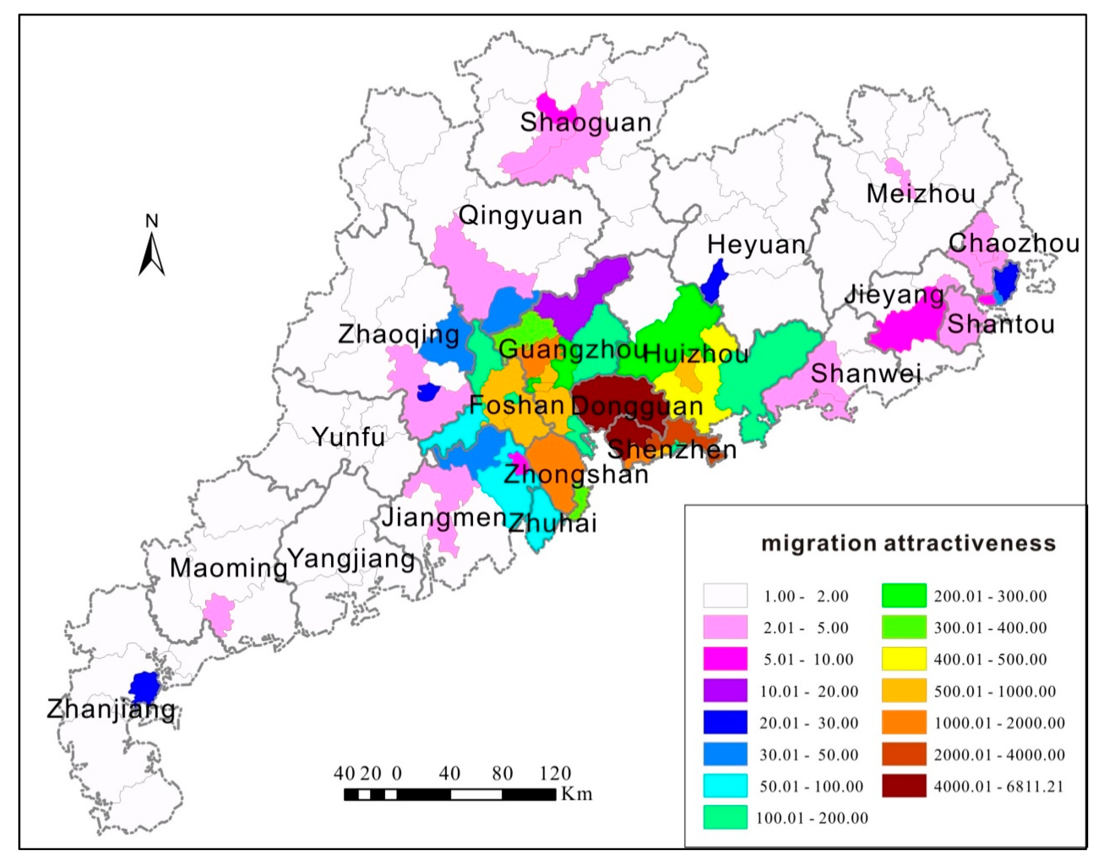
Figure 3.
Scatterplot of in-migrants and relative intrinsic attractivity (RIA) of Guangdong Province.
Figure 3.
Scatterplot of in-migrants and relative intrinsic attractivity (RIA) of Guangdong Province.
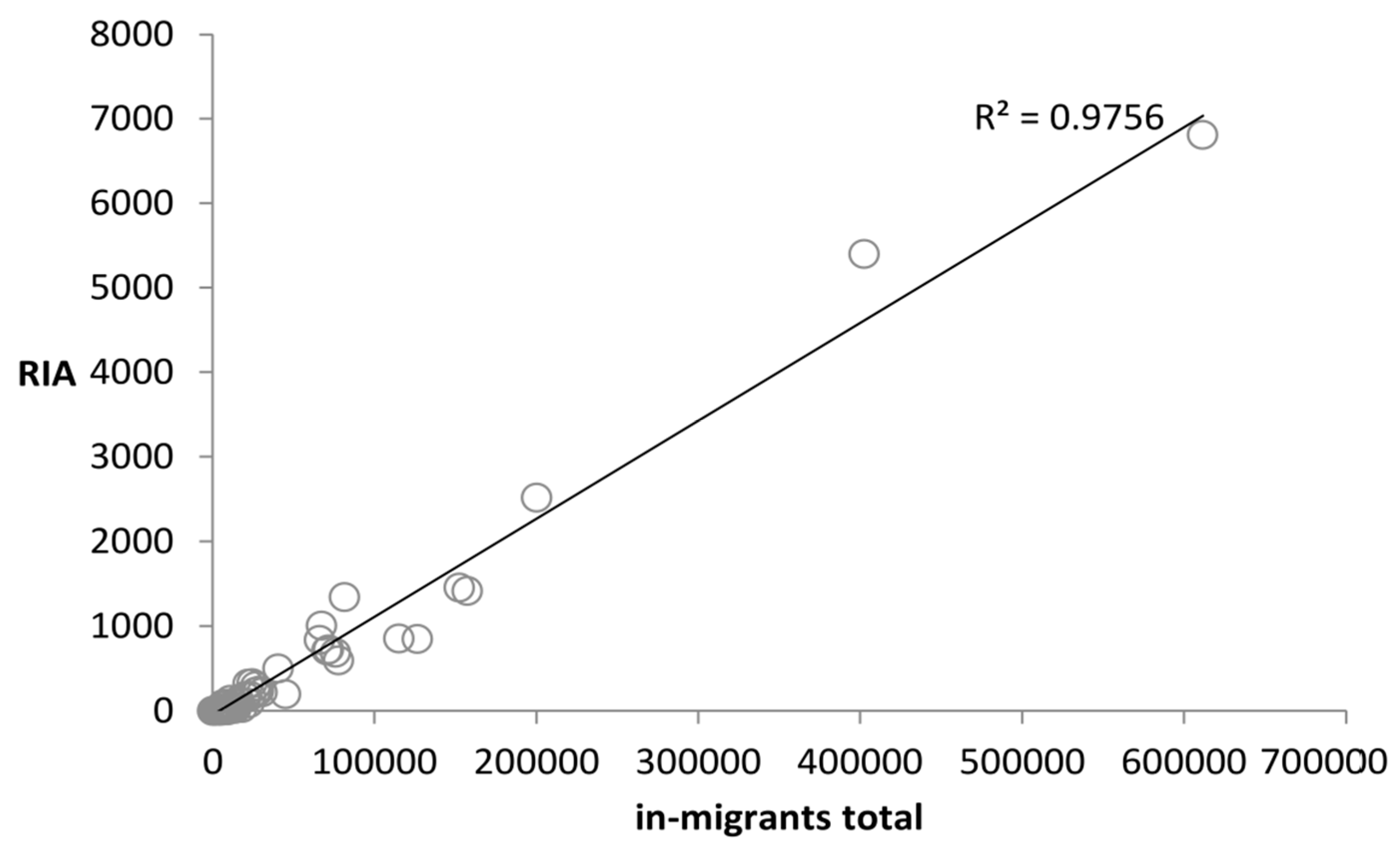
Figure 4.
Local spatial autocorrelation cluster map.

Figure 5.
Ridge trace graph and coefficient of x with k = 0.25.
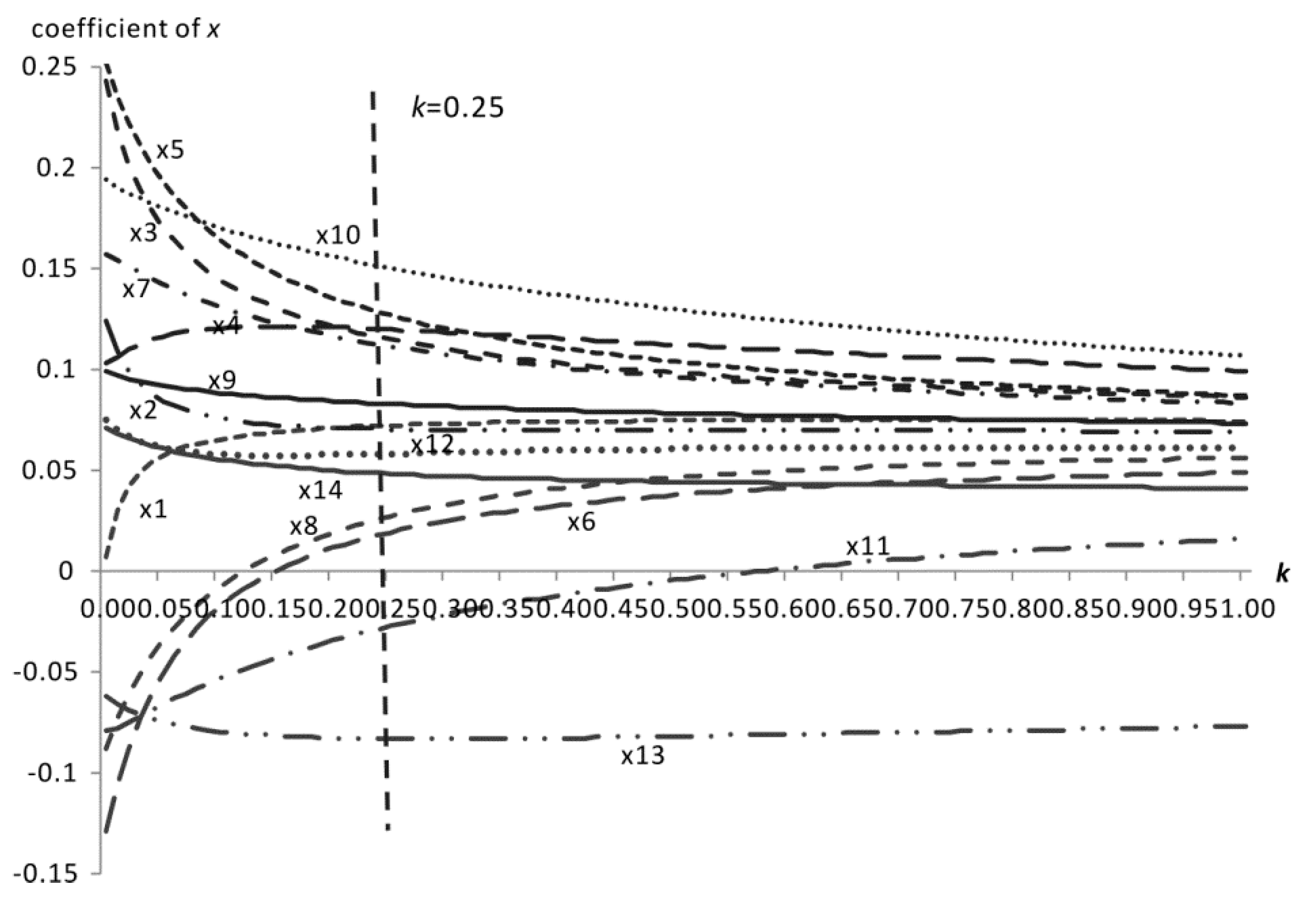
Figure 6.
(A) Histogram of residuals; (B) Residual versus predicted value plot; (C) Residual vs. independent variable (x1); (D) Residual vs. independent variable (x2); (E) Residual vs. independent variable (x3); (F) Residual vs. independent variable (x4); (G) Residual vs. independent variable (x5).
Figure 6.
(A) Histogram of residuals; (B) Residual versus predicted value plot; (C) Residual vs. independent variable (x1); (D) Residual vs. independent variable (x2); (E) Residual vs. independent variable (x3); (F) Residual vs. independent variable (x4); (G) Residual vs. independent variable (x5).

Table 1.
Determinant variables.
| Factors | Variables |
|---|---|
| Economics factors | GDP (x1) |
| Secondary Industrial Output Value (x2) | |
| Tertiary Industrial Output Value (x3) | |
| Per Capital Gross Domestic Product (x4) | |
| Total Investment in Fixed Assets (x5) | |
| Total Retail Sales of Consumer Goods (x6) | |
| the number of industrial enterprises above designated size (x7) | |
| the industrial output value of industrial enterprises above the designated size (x8) | |
| Social service and living standard | the Savings Deposits by Urban and Rural Residents (x9) |
| the Annual Average Wage of Fully Employed Staff and Workers (x10) | |
| the Number of Hospital Beds (x11) | |
| Destination population level | Mean Years of Schooling (x12) |
| Adult illiteracy Rate, Population 15+ years both Sexes (x13) | |
| Labor Force Participation Rate (x14) |
Table 2.
RIA scores: top 30 districts (counties).
| County | Dongguan | Baoan | Longgang | Baiyun | Zhonshan |
|---|---|---|---|---|---|
| RIA | 6811 | 5400 | 2515 | 1452 | 1417 |
| County | Futian | Nanshan | Shunde | Nanhai | Luohu |
| RIA | 1339 | 1002 | 853 | 847 | 838 |
| County | Tianhe | Huicheng | Panyu | Haizhu | Huiyang |
| RIA | 726 | 715 | 683 | 593 | 496 |
| County | Huadu | Xiangzhou | Yuexiu | Huangpu | Boluo |
| RIA | 322 | 318 | 289 | 233 | 223 |
| County | Liwan | Chancheng | Sanshui | Zengcheng | Luogang |
| RIA | 218 | 194 | 175 | 172 | 163 |
| County | Nansha | Huidong | Yantian | Pengjiang | Xinhui |
| RIA | 130 | 123 | 116 | 89 | 82 |
RIA means relative intrinsic attractivity.
Table 3.
Possible 14 determinants and ridge regression statistic.
| Ridge Regression with k = 0.25 | |||||
|---|---|---|---|---|---|
| Mult R | 0.91 | ||||
| RSquare | 0.82 | ||||
| Adj Rsquare | 0.80 | ||||
| SE | 0.45 | ||||
| ANOVA table | |||||
| df | SS | MS | F value | Sig F | |
| Regress | 14 | 98.73 | 7.05 | 35.14 | 0.00 |
| Residual | 106 | 21.27 | 0.20 | ||
| Variables in the Equation | |||||
| B | SE(B) | Beta | T | sig | |
| x1 | 0.0722 | 0.0247 | 0.0722 | 2.9280 | 0.0042 |
| x2 | 0.0705 | 0.0321 | 0.0705 | 2.1973 | 0.0302 |
| x3 | 0.1147 | 0.0335 | 0.1147 | 3.4272 | 0.0009 |
| x4 | 0.1197 | 0.0367 | 0.1197 | 3.2651 | 0.0015 |
| x5 | 0.1266 | 0.0376 | 0.1266 | 3.3687 | 0.0011 |
| x6 | 0.0194 | 0.0336 | 0.0194 | 0.5756 | 0.5661 |
| x7 | 0.1114 | 0.0377 | 0.1114 | 2.9588 | 0.0038 |
| x8 | 0.0272 | 0.0351 | 0.0272 | 0.7753 | 0.4399 |
| x9 | 0.0829 | 0.0375 | 0.0829 | 2.2088 | 0.0293 |
| x10 | 0.1501 | 0.0364 | 0.1501 | 4.1229 | 0.0001 |
| x11 | −0.0274 | 0.0371 | −0.0274 | −0.7378 | 0.4623 |
| x12 | 0.0582 | 0.0357 | 0.0582 | 1.6304 | 0.1060 |
| x13 | −0.0831 | 0.0374 | −0.0831 | −2.2229 | 0.0283 |
| x14 | 0.0482 | 0.0346 | 0.0482 | 1.3944 | 0.1661 |
| Constant | 0.0000 | 0.0407 | 0.0000 | 0.0000 | 1.0000 |
Table 4.
Final 9 statistically significant determinants and statistics.
| Ridge Regression with k = 0.25 | |||||
|---|---|---|---|---|---|
| Mult R | 0.91 | ||||
| RSquare | 0.82 | ||||
| Adj Rsquare | 0.81 | ||||
| SE | 0.44 | ||||
| ANOVA table | |||||
| df | SS | MS | F value | Sig F | |
| Regress | 9 | 98.36 | 10.93 | 56.06 | 0.00 |
| Residual | 111 | 21.64 | 0.20 | ||
| Variables in the Equation | |||||
| B | SE(B) | Beta | T | sig | |
| x1 | 0.0811 | 0.0265 | 0.0811 | 3.0640 | 0.0027 |
| x2 | 0.0822 | 0.0349 | 0.0822 | 2.3573 | 0.0202 |
| x3 | 0.1195 | 0.0340 | 0.1195 | 3.5156 | 0.0006 |
| x4 | 0.1466 | 0.0366 | 0.1466 | 4.0018 | 0.0001 |
| x5 | 0.1184 | 0.0377 | 0.1184 | 3.1379 | 0.0022 |
| x7 | 0.1092 | 0.0368 | 0.1092 | 2.9650 | 0.0037 |
| x9 | 0.0919 | 0.0371 | 0.0919 | 2.4760 | 0.0148 |
| x10 | 0.1567 | 0.0356 | 0.1567 | 4.3991 | 0.0000 |
| x13 | −0.1157 | 0.0375 | −0.1157 | −3.0885 | 0.0025 |
| Constant | 0.0000 | 0.0401 | 0.0000 | 0.0000 | 1.0000 |
© 2019 by the authors. Licensee MDPI, Basel, Switzerland. This article is an open access article distributed under the terms and conditions of the Creative Commons Attribution (CC BY) license (http://creativecommons.org/licenses/by/4.0/).
Share and Cite
MDPI and ACS Style
Yang, Q.; Zhang, H.; M Mwenda, K. County-Scale Destination Migration Attractivity Measurement and Determinants Analysis: A Case Study of Guangdong Province, China. Sustainability 2019, 11, 362. https://doi.org/10.3390/su11020362
AMA Style
Yang Q, Zhang H, M Mwenda K. County-Scale Destination Migration Attractivity Measurement and Determinants Analysis: A Case Study of Guangdong Province, China. Sustainability. 2019; 11(2):362. https://doi.org/10.3390/su11020362
Chicago/Turabian StyleYang, Qingsheng, Hongxian Zhang, and Kevin M Mwenda. 2019. "County-Scale Destination Migration Attractivity Measurement and Determinants Analysis: A Case Study of Guangdong Province, China" Sustainability 11, no. 2: 362. https://doi.org/10.3390/su11020362
Note that from the first issue of 2016, this journal uses article numbers instead of page numbers. See further details here.