Investigation for the Decomposition of Carbon Emissions in the USA with C-D Function and LMDI Methods

Abstract

Residual problems are one of the greatest challenges in developing new decomposition techniques, especially when combined with the Cobb–Douglas (C-D) production function and the Logarithmic Mean Divisia Index (LMDI) method. Although this combination technique can quantify more effects than LMDI alone, its decomposition result has residual value. We propose a new approach that can achieve non-residual decomposition by calculating the actual values of three key parameters. To test the proposed approach, we decomposed the carbon emissions in the United States to six driving factors: the labor input effect, the investment effect, the carbon coefficient effect, the energy structure effect, the energy intensity effect, and the technology state effect. The results illustrate that the sum of these factors is equivalent to the CO₂ emissions changes from t to t-1, thereby proving non-residual decomposition. Given that the proposed approach can achieve perfect decomposition, the proposed approach can be used more widely to investigate the effects of labor input, investment, and technology state on changes in energy and emission.

1. Introduction

When exploring the factors affecting energy consumption or carbon emissions, it is the pursuit of more scholars to decompose more factors. However, the factors that can be decomposed by using a single decomposition method are limited. In order to explore more drivers, many scholars have adopted a way to combine decomposition models with other economic models. To quantify the effects of fixed asset investment and labor input on changes in energy consumption and carbon emissions, Wang et al. [1] combined the Cobb–Douglas (C-D) production function and the Logarithmic Mean Divisia Index (LMDI) econometric method. This combined technique can quantify more effects than can LMDI alone. However, the results of the decomposition using this technique have residual problems, which means that the technique cannot solve the zero-value problem or implement perfect decomposition. In a recent study, Dong et al. [2] confessed that the combination technique could not implement complete decomposition, but nevertheless, was still applied, because this technique was able to quantify the effects of labor force input and fixed asset investment on changes in carbon emissions. However, the combined decomposition technique with residuals will result in inaccurate results, which will reduce the credibility of the conclusions. Therefore, the purpose of this paper is to solve the residual problem and achieve perfect decomposition of the combination technique and to conduct empirical analysis based on US carbon emissions. Guided by applied intermediate macroeconomics [3], this paper reports a new approach to solving the zero-value problem and exploring one more factor, which is the technology state factor. In this way, the combined decomposition technique can be better used in studying the effects of fixed asset investment, labor force input and technology state on energy consumption changes and carbon emissions changes.

The remainder of this paper is structured as follows. Section 2 is a literature review of decomposition techniques. Section 3 presents the proposed approach to using the combined decomposition technique to achieve perfect decomposition. Section 4 describes the testing of the proposed approach by decomposing CO2 emissions in the United States. Finally, Section 5 concludes this paper.

2. Literature Review

Generally, there are two primary categories of the decomposition method: structural decomposition analysis (SDA) and index decomposition analysis (IDA) [1,4]. The SDA method, which is based upon the input–output tables, is widely used to analyze the influencing factors driving the energy consumption and energy-related emissions changes [5,6,7,8,9,10]. For CO₂ emissions in Spain, José M. Cansino et al. used SDA to decompose the changes into six effects [11]. Bin Su et al. [12] and Jing Wei et al. [13] also employed SDA to analyze the influencing factors of CO2 emission changes in Singapore and Beijing. Zhu et al. utilized an input–output framework and SDA method to explore the driving forces for the changes in India’s total emissions and intensity [14]. However, input–output tables are not always readily available, thereby limiting the widespread use of SDA [5,15]. Wang et al. compared the application of the SDA method and IDA method in energy consumption and energy-related emissions research from the viewpoints of methodology and application [16]. Xu and Ang reviewed and summarized 80 papers that applied the IDA method on emission studies during 1991 to 2012, and the results revealed that IDA is more widely used than SDA when decomposed CO₂ emissions change [17]; and then, they employed the IDA method to decompose the residential energy consumption in Singapore [18]. The IDA method can be separated into two approaches: the Laspeyres Index approach and the Divisia Index approach [19,20,21]. The Laspeyres Index approach has rarely been used to analyze carbon emissions due to the residual problem [22]. The Divisia Index approach was first proposed by Boyd and included the Arithmetic Mean Divisia Index (AMDI) and Logarithmic Mean Divisia Index (LMDI) methods. LMDI is more extensively utilized because AMDI results in incomplete decomposition and zero-value problems [23,24]. Based on the expansion and improvement of the Divisia Index method by previous research [25,26,27,28,29], LMDI has become the preferred method for decomposing CO₂ emissions [23,30]. To solve zero-value problems, Ang and Liu have put forward eight strategies [31]. Moreover, Ang summarized the basic formulas for the eight LMDI models and made comparisons between these models, and then developed model selection guidelines for potential users [32].

LMDI has been adopted by many academics to investigate the decomposition of CO₂ emissions at national levels [33,34], provincial levels [35,36,37] and the levels of specific industries [16,38] such as the chemical industry [22], construction industry [39,40], manufacturing industry [41], heavy industry [42], logistics Industry [43], and power industry [9], as well as at the levels of the whole of industry [44]. Akbostanci et al. applied LMDI to decompose the CO₂ emissions of the Turkish manufacturing industry into five influencing factors: overall activity, economy structure, sectoral energy intensity, sectoral energy structure, and CO₂ emission coefficient [45]. Babak Mousavi et al. analyzed the influencing factors driving Iran’s CO₂ emission changes [46]. Jeong et al. decomposed the CO₂ emissions from South Korean industrial manufacturing into five influencing factors: economic activity, economic structure, energy intensity, energy-mix, and emission-factor [47]. Achour et al. calculated the contributions of the transportation intensity, energy intensity, economic output, population scale effect, and transportation structure effect of the Tunisian transportation sector [48]. Zhao et al. used LMDI method to decompose CO₂ emissions in Guangdong Province from a sector perspective, and the results showed that the energy intensity effect and economic output effect were the critical factors for carbon emissions in Guangdong Province [37]. Wang et al. used the LMDI model and Tapio decoupling model to study the influencing factors of decoupling status between CO₂ emissions and economy from the city level, and the results showed that the economic effect and population effect inhibited the decoupling and energy intensity accelerated the decoupling [16]. It can be concluded that the research objects have been divided very carefully in the above research using LMDI to explore the decomposition of CO₂ emissions, but there is seldom innovation in the driving factors. To explore the contributions of the fixed asset investment and labor factors to China’s energy consumption changes, Wang et al. proposed a decomposition technique combining the C-D production function and LMDI [1]. The results illustrated that the factors of fixed asset investment and labor were critical to influencing energy consumption. Moreover, Dong et al. used the combined decomposition technique to analyze energy consumption in Liaoning Province and showed that the fixed asset investment effect played a negative role while the labor effect played a very weak role in the phenomenon of decoupling [2].

By reviewing the development of the decomposition method, it can be seen that the combination of the C-D production function and LMDI can decompose the effects of labor force input and fixed asset investment on changes in energy consumption and carbon emissions. However, this combined decomposition technique caused incomplete decomposition and had residuals in its results. Moreover, the combined decomposition technique ignored the effect of the technology state. In this paper, the proposed approach is aimed at solving the residual value of the combined decomposition technique.

3. Proposed Approach to Achieve Complete Decomposition

When applying the LMDI method, the total CO₂ emissions can always be expressed in the traditional decomposition form [49,50]. The traditional influencing factors include the carbon coefficient, energy structure, energy intensity, and economic outputs. The function is as follows:

$${\mathit{C}}_{\mathit{t}}={\displaystyle \mathit{\sum }}_{\mathit{i}=\mathit{1}}^{\mathit{3}}\frac{{\mathit{C}}_{\mathit{i}\mathit{t}}}{{\mathit{E}}_{\mathit{i}\mathit{t}}}\mathit{\times }\frac{{\mathit{E}}_{\mathit{i}\mathit{t}}}{{\mathit{E}}_{\mathit{t}}}\mathit{\times }\frac{{\mathit{E}}_{\mathit{t}}}{\mathit{G}\mathit{D}{\mathit{P}}_{\mathit{t}}}\mathit{\times }\mathit{G}\mathit{D}{\mathit{P}}_{\mathit{t}}$$

(1)

$$={\displaystyle \mathit{\sum }}_{\mathit{i}=\mathit{1}}^{\mathbf{3}}{\mathit{F}}_{\mathit{i}\mathit{t}}\mathit{\times }{\mathit{S}}_{\mathit{i}\mathit{t}}\mathit{\times }{\mathit{I}}_{\mathit{t}}\mathit{\times }\mathit{G}\mathit{D}{\mathit{P}}_{\mathit{t}}$$

(2)

where t denotes the time in years; i denotes energy type; ${\mathit{C}}_{\mathit{t}}$ and ${\mathit{C}}_{\mathit{i}\mathit{t}}$ denote, respectively, the total CO₂ emissions and the CO₂ emissions of the i-th energy type in t year; ${\mathit{E}}_{\mathit{t}}$ and ${\mathit{E}}_{\mathit{i}\mathit{t}}$ denote, respectively, the total energy consumption and the consumption of the ith energy in year t; $\mathit{G}\mathit{D}{\mathit{P}}_{\mathit{t}}$ denotes the gross domestic product in year t; ${\mathit{F}}_{\mathit{i}\mathit{t}}=\frac{{\mathit{C}}_{\mathit{i}\mathit{t}}}{{\mathit{E}}_{\mathit{i}\mathit{t}}}$ denotes the carbon coefficient of the i-th energy in year t; $S_{it}=\frac{{\mathit{E}}_{\mathit{i}\mathit{t}}}{{\mathit{E}}_{\mathit{t}}}$ denotes the energy structure of the i-th energy in year t; and $I_t=\frac{E_t}{Q_t}$ denotes energy intensity in year t.

The above analysis shows that the traditional decomposition form cannot reflect the impacts of fixed asset investment and labor on carbon emissions. Building on previous research and economic theory, Wang et al. [1] combined the C-D production function and LMDI to formulate the proposed combined decomposition technique. The C-D production function is a particularly useful one in many mathematical functions, because it has the production function properties that we expect and has been extended to the field of economics by Paul Douglas and Charles Cobb. In particular, the C-D production function describes how the real economy transforms fixed asset investment and labor into GDP. So, we can use the C-D production function, which is shown below, to describe GDP:

$$\mathit{G}\mathit{D}{\mathit{P}}_{\mathit{t}}=\mathit{A}{\left({\mathit{L}}_{\mathit{t}}\right)}^{\mathit{\alpha }}{\left({\mathit{K}}_{\mathit{t}}\right)}^{\mathit{\beta }}$$

(3)

Putting Equation (3) into the GDP on the right-hand side of Equation (2), a new form of decomposition can be obtained:

$${\mathit{C}}_{\mathit{t}}={\displaystyle \mathit{\sum }}_{\mathit{i}=\mathbf{1}}^{\mathbf{3}}{\mathit{F}}_{\mathit{i}\mathit{t}}\mathit{\times }{\mathit{S}}_{\mathit{i}\mathit{t}}\mathit{\times }{\mathit{I}}_{\mathit{t}}\mathit{\times }\mathit{A}\mathit{\times }{\left({\mathit{L}}_{\mathit{t}}\right)}^{\mathit{\alpha }}\mathit{\times }{\left({\mathit{K}}_{\mathit{t}}\right)}^{\mathit{\beta }}\mathit{ }$$

(4)

where A is a positive constant that can be treated as a target of the state of technology; $\alpha \mathrm{and} \beta$ are unknown constant parameters while $\alpha +\beta =1$; and ${\mathit{L}}_{\mathit{t}}$ and ${\mathit{K}}_{\mathit{t}}$ denote the amount of labor input and fixed asset investment, respectively, in year t.

According to Ang, by using the additive form, the change in CO₂ emissions ($\mathit{\Delta }{\mathit{C}}_{\mathit{t}}$) between a base year 0 and a target year t can be decomposed into the six influencing factors: the carbon coefficient effect ($\mathit{\Delta }{\mathit{C}}_{\mathit{F}\mathit{t}}$), the energy structure effect ($\mathit{\Delta }{\mathit{C}}_{\mathit{S}\mathit{t}}$), the energy intensity effect ($\mathit{\Delta }{\mathit{C}}_{\mathit{I}\mathit{t}}$), the technology state effect ($\mathit{\Delta }{\mathit{C}}_{\mathit{A}\mathit{t}}$), the labor input effect ($\mathit{\Delta }{\mathit{C}}_{\mathit{L}\mathit{t}}$), and the investment effect ($\mathit{\Delta }{\mathit{C}}_{\mathit{K}\mathit{t}}$). The function is shown below:

$$\mathbf{\Delta }{\mathit{C}}_{\mathit{t}}={\mathit{C}}_{\mathit{t}}\mathit{-}{\mathit{C}}_{\mathbf{0}}=\mathbf{\Delta }{\mathit{C}}_{\mathit{F}\mathit{t}}+\mathbf{\Delta }{\mathit{C}}_{\mathit{S}\mathit{t}}+\mathbf{\Delta }{\mathit{C}}_{\mathit{I}\mathit{t}}+\mathbf{\Delta }{\mathit{C}}_{\mathit{A}\mathit{t}}+\mathbf{\Delta }{\mathit{C}}_{\mathit{L}\mathit{t}}+\mathbf{\Delta }{\mathit{C}}_{\mathit{K}\mathit{t}}$$

(5)

According to LMDI, each effect can be computed as follows:

$$\mathbf{\Delta }{\mathit{C}}_{\mathit{F}\mathit{t}}={\displaystyle \sum }_{i=1}^3(\frac{C_{it}-C_{i0}}{ln{C}_{it}-ln{C}_{i0}}\times ln\frac{F_{it}}{F_{i0}})$$

$$\mathbf{\Delta }{\mathit{C}}_{\mathit{S}\mathit{t}}={\displaystyle \sum }_{i=1}^3(\frac{C_{it}-C_{i0}}{ln{C}_{it}-ln{C}_{i0}}\times ln\frac{S_{it}}{S_{i0}})$$

$$\mathbf{\Delta }{\mathit{C}}_{\mathit{I}\mathit{t}}={\displaystyle \sum }_{i=1}^3(\frac{C_{it}-C_{i0}}{ln{C}_{it}-ln{C}_{i0}}\times ln\frac{I_t}{I_0})$$

$$\mathbf{\Delta }{\mathit{C}}_{\mathit{A}\mathit{t}}={\displaystyle \sum }_{i=1}^3(\frac{C_{it}-C_{i0}}{ln{C}_{it}-ln{C}_{i0}}\times ln\frac{A_t}{A_0})$$

$$\mathbf{\Delta }{\mathit{C}}_{\mathit{L}\mathit{t}}={\displaystyle \sum }_{i=1}^3(\frac{C_{it}-C_{i0}}{ln{C}_{it}-ln{C}_{i0}}\times ln\frac{{(L_t)}^{\alpha }}{{(L_0)}^{\alpha }})$$

$$\mathbf{\Delta }{\mathit{C}}_{\mathit{K}\mathit{t}}={\displaystyle \sum }_{i=1}^3(\frac{C_{it}-C_{i0}}{ln{C}_{it}-ln{C}_{i0}}\times ln\frac{{(K_t)}^{\beta }}{{(K_0)}^{\beta }})$$

The combined decomposition technique ignored the actual values of $A,\alpha \mathrm{and} \beta$ and treated them as unknown constants for computational convenience. Thus, $\ln \left(A_t/A_0\right)=0$ and $\Delta C_{At}=0$ [1,2]. In conclusion, the combined decomposition technique not only has residuals in its results but also ignores the effect of the technology state. In this paper, the actual values of $A,\alpha \mathrm{and} \beta$ are calculated according to Kevin D. Hoover’s applied intermediate macroeconomics [3]. Thus, non-residual decomposition is realized and the technology state factor is quantified. The calculation steps are as follows:

According to Equation (3) and $\alpha +\beta =1$, the C-D production function can be written as:

$$\mathit{Y}=\mathit{A}{\left(\mathit{L}\right)}^{\mathit{\alpha }}{\left(\mathit{K}\right)}^{\mathbf{1}\mathit{-}\mathit{\alpha }}$$

(6)

Calculating the derivatives of K and L for Y, we obtain the marginal product of labor input ($\mathit{m}\mathit{p}\mathit{L}$) and the marginal product of physical capital ($\mathit{m}\mathit{p}\mathit{K}$), respectively. The function is shown below:

$$\mathit{m}\mathit{p}\mathit{L}=\mathit{\alpha }\mathit{\times }\mathit{A}\mathit{\times }{\left(\frac{\mathit{K}}{\mathit{L}}\right)}^{\mathbf{1}\mathit{-}\mathit{\alpha }}=\mathit{\alpha }\mathit{\times }\frac{\mathit{Y}}{\mathit{L}}$$

(7)

$$\mathit{m}\mathit{p}\mathit{K}=\left(\mathbf{1}\mathit{-}\mathit{\alpha }\right)\mathit{\times }\mathit{A}\mathit{\times }{\left(\frac{\mathit{L}}{\mathit{K}}\right)}^{\mathit{\alpha }}=\left(\mathbf{1}\mathit{-}\mathit{\alpha }\right)\mathit{\times }\frac{\mathit{Y}}{\mathit{K}}$$

(8)

In economics, real labor income $\left({\mathit{Y}}_{\mathit{L}}\right)$ is the product of the real wage rate $\left(\mathit{\omega }/\mathit{p}\right)$ and the number of hours worked $\left(\mathit{L}\right)$:

$${\mathit{Y}}_{\mathit{L}}=\left(\mathit{\omega }/\mathit{p}\right)\mathit{\times }\mathit{L}$$

(9)

where $\mathit{\omega }$ is the wage rate and $\mathit{p}$ is the market price.

$$\mathit{L}\mathit{-}\mathit{s}\mathit{h}\mathit{a}\mathit{r}\mathit{e}=\left(\frac{{\mathit{Y}}_{\mathit{L}}}{\mathit{Y}}\right)=\left(\frac{\mathit{\omega }}{\mathit{p}}\right)\mathit{\times }\frac{\mathit{L}}{\mathit{Y}}$$

(10)

where $\mathit{L}\mathit{-}\mathit{s}\mathit{h}\mathit{a}\mathit{r}\mathit{e}$ is the labor share; and ${\mathit{Y}}_{\mathit{L}}$ and $\mathit{Y}$ denote the real labor income and the total income, respectively.

Similarly, the real capital income $\left({\mathit{Y}}_{\mathit{K}}\right)$ and the capital share $\left(\mathit{K}\mathit{-}\mathit{s}\mathit{h}\mathit{a}\mathit{r}\mathit{e}\right)$ are defined as follows:

$${\mathit{Y}}_{\mathit{k}}=\left(\mathit{\nu }/\mathit{p}\right)\mathit{\times }\mathit{K}$$

(11)

$$\mathit{K}\mathit{-}\mathit{s}\mathit{h}\mathit{a}\mathit{r}\mathit{e}=\left(\frac{{\mathit{Y}}_{\mathit{K}}}{\mathit{Y}}\right)=\left(\mathit{\nu }/\mathit{p}\right)\mathit{\times }\frac{\mathit{K}}{\mathit{Y}}$$

(12)

where $\mathit{\nu }$ is the rental rate; $\mathit{p}$ is the market price; $\left(\mathit{\nu }/\mathit{p}\right)$ is the real rental rate; and $\mathit{K}$ is the amount of fixed asset investment.

To further explain these definitions, we apply the assumption that the economy is close to perfect competition. Under this assumption, we can use the profit maximization rules, which state that each real factor price is equivalent to the corresponding marginal product. The functions are shown below:

$$\mathit{m}\mathit{p}\mathit{L}=\frac{\mathbf{\Delta }\mathit{Y}}{\mathbf{\Delta }\mathit{L}}=\mathit{\omega }/\mathit{p}$$

(13)

$$\mathit{m}\mathit{p}\mathit{K}=\frac{\mathbf{\Delta }\mathit{Y}}{\mathbf{\Delta }\mathit{K}}=\mathit{\nu }/\mathit{p}$$

(14)

Replacing the factor prices with the marginal products in Equations (10) and (12):

$$\mathit{L}\mathit{-}\mathit{s}\mathit{h}\mathit{a}\mathit{r}\mathit{e}=\left(\frac{{\mathit{Y}}_{\mathit{L}}}{\mathit{Y}}\right)=\left(\mathit{m}\mathit{p}\mathit{L}\right)\mathit{\times }\frac{\mathit{L}}{\mathit{Y}}$$

(15)

$$\mathit{K}\mathit{-}\mathit{s}\mathit{h}\mathit{a}\mathit{r}\mathit{e}=\left(\frac{{\mathit{Y}}_{\mathit{L}}}{\mathit{K}}\right)=\left(\mathit{m}\mathit{p}\mathit{K}\right)\mathit{\times }\frac{\mathit{K}}{\mathit{Y}}$$

(16)

We can replace mpL and mpK in Equations (15) and (16) with the specific forms in Equations (7) and (8). The functions are shown below:

$$\mathit{L}\mathit{-}\mathit{s}\mathit{h}\mathit{a}\mathit{r}\mathit{e}=\left(\frac{{\mathit{Y}}_{\mathit{L}}}{\mathit{Y}}\right)=\left(\mathit{\alpha }\mathit{\times }\frac{\mathit{Y}}{\mathit{L}}\right)\mathit{\times }\frac{\mathit{L}}{\mathit{Y}}=\mathit{\alpha }$$

(17)

$$\mathit{K}\mathit{-}\mathit{s}\mathit{h}\mathit{a}\mathit{r}\mathit{e}=\left(\frac{{\mathit{Y}}_{\mathit{L}}}{\mathit{K}}\right)=\left(\left(\mathbf{1}\mathit{-}\mathit{\alpha }\right)\mathit{\times }\frac{\mathit{Y}}{\mathit{K}}\right)\mathit{\times }\frac{\mathit{K}}{\mathit{Y}}=\mathbf{1}\mathit{-}\mathit{\alpha }$$

(18)

From the above analysis, we can draw the conclusion that the indexes of L and K in the C-D production function ($\alpha ,\beta$) are equal to the labor and capital shares, respectively. So, we can calculate the actual value of $\alpha$ by calculating the labor share with the following function:

$$\mathit{\alpha }=\mathit{L}\mathit{-}\mathit{s}\mathit{h}\mathit{a}\mathit{r}\mathit{e}=\frac{\mathit{c}\mathit{o}\mathit{m}\mathit{p}\mathit{e}\mathit{n}\mathit{s}\mathit{a}\mathit{t}\mathit{i}\mathit{o}\mathit{n}\mathit{ }\mathit{o}\mathit{f}\mathit{ }\mathit{e}\mathit{m}\mathit{p}\mathit{l}\mathit{o}\mathit{y}\mathit{e}\mathit{e}\mathit{s}}{\mathit{t}\mathit{o}\mathit{t}\mathit{a}\mathit{l}\mathit{ }\mathit{i}\mathit{n}\mathit{c}\mathit{o}\mathit{m}\mathit{e}}$$

(19)

$$\mathit{\beta }=\mathit{K}\mathit{-}\mathit{s}\mathit{h}\mathit{a}\mathit{r}\mathit{e}=\mathbf{1}\mathit{-}\mathit{\alpha }$$

(20)

where total income includes the compensation of employees, rental income of persons, corporate profits, net interest, miscellaneous payments, and depreciation value.

When the actual value of $\alpha$ was calculated and the data of the labor force and capital were obtained, the current year’s technology state index $\left(\mathit{A}\right)$ can be calculated using the following formula:

$$\mathit{A}=\frac{\mathit{Y}}{{\left(\mathit{L}\right)}^{\mathit{\alpha }}{\left(\mathit{K}\right)}^{\mathbf{1}\mathit{-}\mathit{\alpha }}}$$

(21)

4. Empirical Analysis

To test if the proposed approach implements non-residual decomposition, the carbon emissions in the United States have been selected for empirical analysis. To clearly demonstrate the issue of perfect decomposition, we conducted a comparative analysis of the traditional approach and proposed approach.

4.1. Data Collection

The data about energy consumption and emissions were derived from the US Energy Information Administration (EIA) [51]. The labor force data was from the US Bureau of Labor Statistics (BLS) [52]. The GDP and real net stock of fixed assets, which have been converted to 2009 constant dollars, were from the US Bureau of Economic Analysis (BEA) [53]. The research period started from 2000 and ended in 2016.

4.2. Traditional Approach

According to the traditional approach [1,2], $A,\alpha \mathrm{and} \beta$ are unknown constant parameters, so $\ln \left(A_t/A_0\right)=0$ and $\Delta C_{At}=0$. It can be concluded that the constant A has no influence on the USA’s carbon emissions.

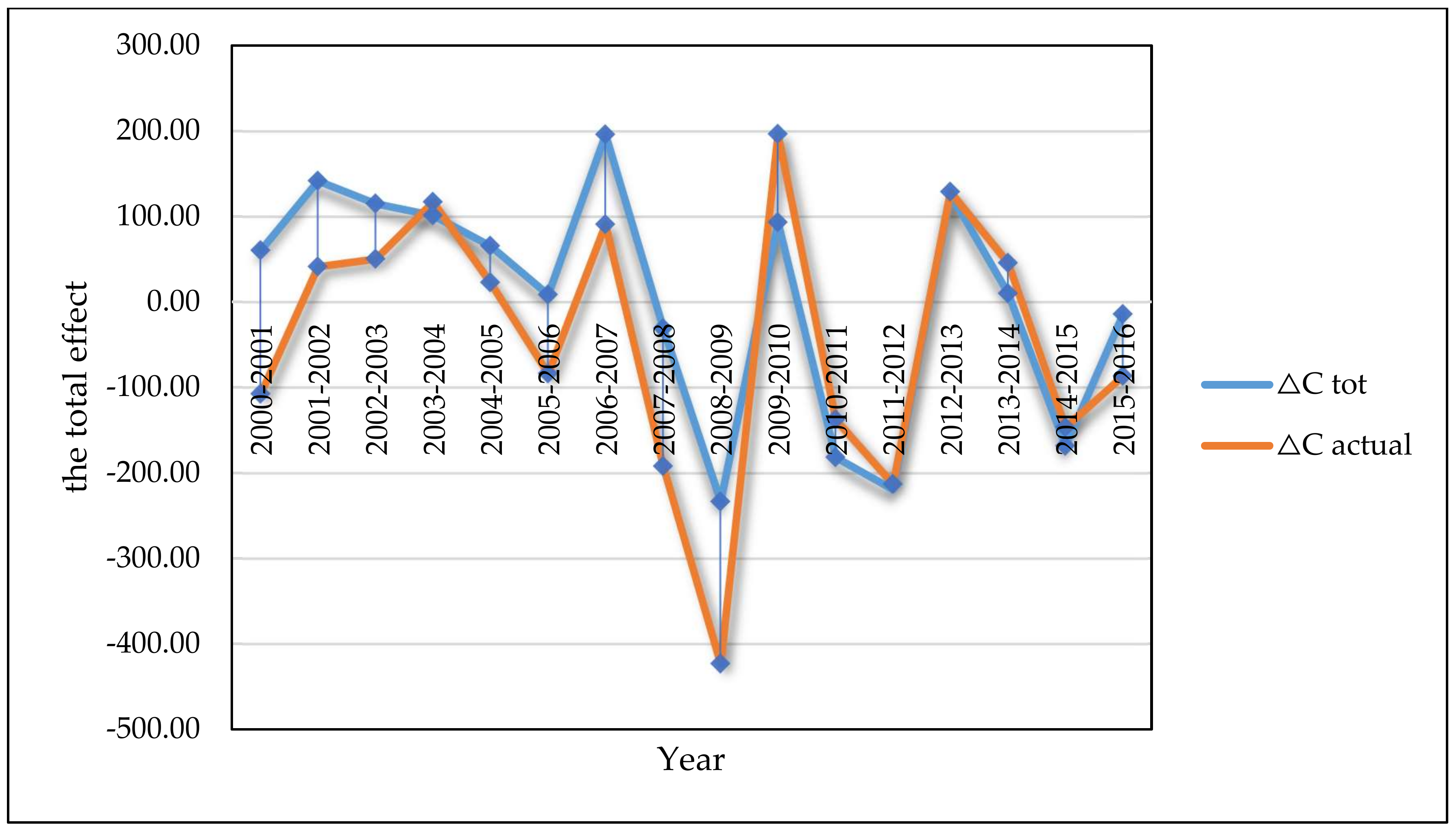
Using Equations (1)–(5), the effects of the five influencing factors can be obtained. The results of the decomposition using the combined decomposition technique are shown in

Table 1. Decomposition results under the traditional approach (unit: Million Metric Tons).

Year	ΔCFt	ΔCSt	ΔCIt	ΔCKt	ΔCLt	ΔCtot	ΔCactual
2000–2001	15,893	1.003	−180,539	177,222	46,659	60,238	−107,315
2001–2002	1.411	−13,073	−49,302	157,527	45,149	141,713	41,232
2002–2003	9.477	19,956	−140,047	159,936	65,754	115,076	50,378
2003–2004	5.263	−4.827	−102,687	167,982	35,771	101,502	116,974
2004–2005	5.170	14,480	−193,020	162,028	77,223	65,880	23,053
2005–2006	−1.941	−1.020	−236,972	165,472	83,268	8.806	−83,605
2006–2007	8.886	−15.262	−7.676	143,823	66,192	195,964	90,714
2007–2008	1.813	−0.945	−175,539	99,006	44,581	−31,083	−191,848
2008–2009	−16,475	−55,218	−194,149	37,848	−5.248	−233,242	−422,989
2009–2010	−7.334	8.974	58,076	42,451	−8.988	93,179	196,535
2010–2011	−2.434	−35,095	−187,356	53,242	−9.732	−181,375	−137,469
2011–2012	−1.947	−77,848	−250,248	64,174	46,858	−219,012	−212,956
2012–2013	−10,620	5.944	45,741	71,518	14,098	126,680	128,982
2013–2014	3.009	−10,542	−83,002	82,173	18,394	10,033	45,733
2014–2015	−2.531	−83,132	−210,671	86,779	41,047	−168,509	−146,286
2015–2016	−0.101	−42,790	−120,131	81,144	67,689	−14,189	−86,274
2000–2016	7.537	−289.39	−2027.522	1752.33	628,716	71,662	−695,141

. The comparison of the actual values to the decomposition values is shown in Figure 1. As shown in Table 1, the critical factors that impacted CO₂ emissions in the United States was the energy intensity effect and the investment effect, which were the largest inhibitor and contributor. In terms of cumulative effects, the investment effect has contributed to the growth of 1752.33 million metric tons of CO2 emissions, while the energy intensity effect has inhibited the growth of 2027.52 million tons of CO2 emissions. The investment effect and the labor input effect always played a positive role in the growth of CO₂ emissions during 2000–2016, and the effect of the carbon coefficient, the energy structure and the energy intensity on the growth of CO₂ emissions changed over time. From the perspective of cumulative effects, the energy structure effect was the second inhibitor for the growth of CO₂ emissions, which has inhibited the growth of 289.39 million tons of CO₂ emissions; while the labor input effect was the second contributor, which has contributed to the growth of 628.71 million metric tons of CO₂ emissions. As for the carbon coefficient effect, its role is very weak.

However, by comparing the total effects of decomposition and the actual values, it can be found that there were residuals in this decomposition mode. As shown in Figure 1, the total effects of decomposition were not much different from the actual values in 2003–2004 and 2010–2015, but they were not completely equal. In 2001–2003, 2004–2010 and 2015–2016, the difference between the total effects and the actual values was very large. It is worth noting that in 2000–2001 and 2005–2006, the US carbon dioxide emissions showed a downward trend, while the total effects of decomposition were positive. It can be concluded that there were residuals in the decomposition results resulting from the fact that the actual values of $A,\alpha \mathrm{and} \beta$ were neglected. Furthermore, the decomposition method with residuals will reduce the credibility of the conclusion and result in inaccurate analysis, which are not conducive to the effectiveness of policy implementation.

4.3. The Proposed Approach

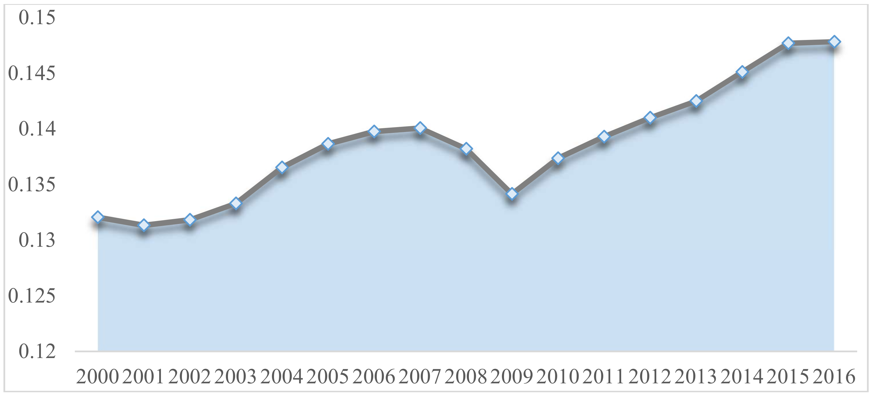
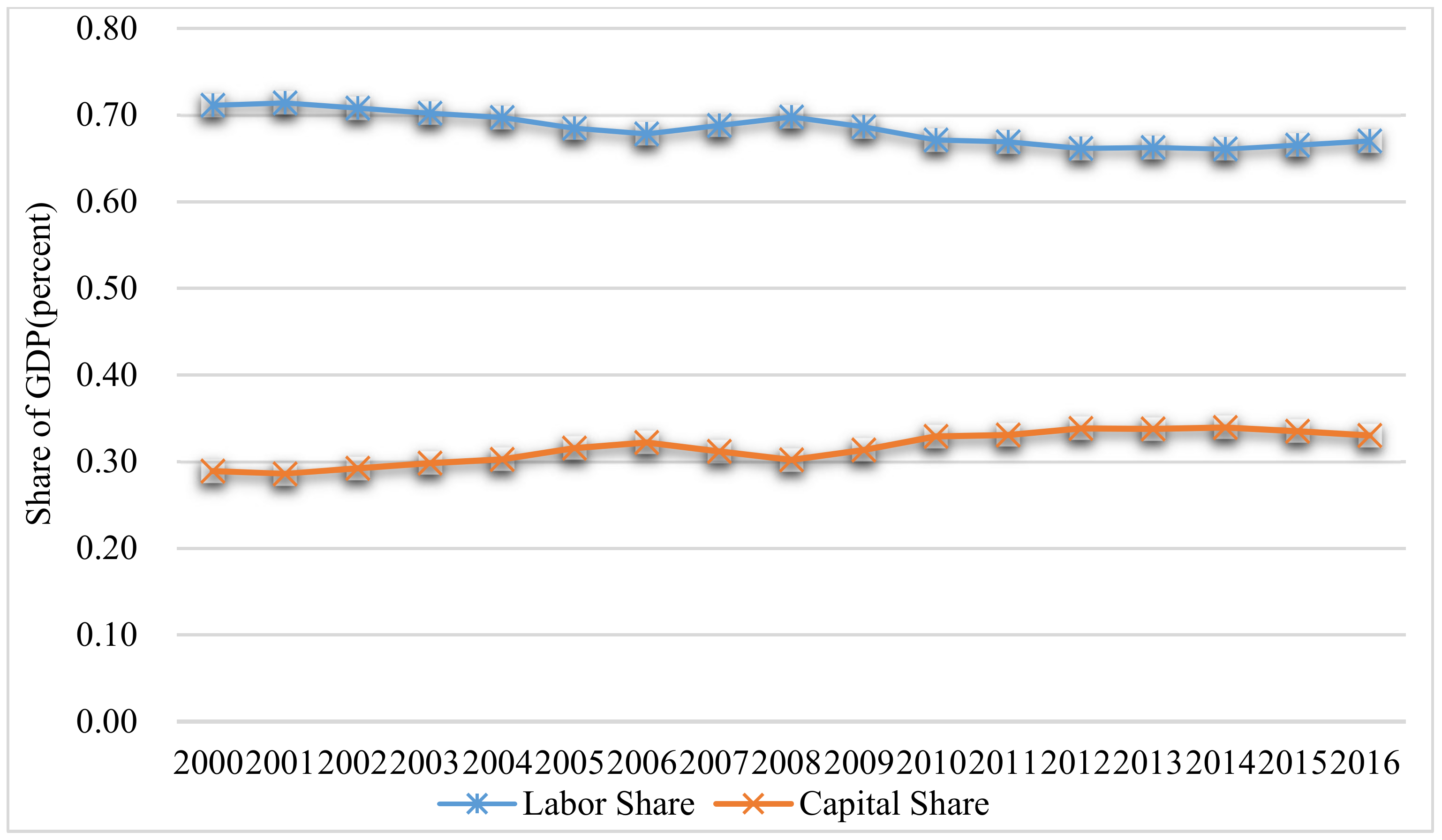
According to the proposed approach, the actual values of $\mathrm{A},\alpha \mathrm{and} \beta$ can be calculated using Equations (16)–(18). As shown in Figure 2, the labor share and capital share change about a mean that is nearly constant from year to year and is regarded as an estimate of $\alpha$, so $\alpha =0.68 \mathrm{and} \beta =0.32$. The index of the technology state (A) is shown in Figure 3. It can be seen that the technology state in the USA has an upward trend in volatility from 2000 to 2016, but there was a decline from 2007 to 2009.

After calculating the value of each parameter, the USA’s emissions can be decomposed into six influencing factors: the carbon coefficient effect ($\mathbf{\Delta }{\mathit{C}}_{\mathit{F}\mathit{t}}$), the energy structure effect ($\mathbf{\Delta }{\mathit{C}}_{\mathit{S}\mathit{t}}$), the energy intensity effect ($\mathbf{\Delta }{\mathit{C}}_{\mathit{I}\mathit{t}}$), the technology state effect ($\mathbf{\Delta }{\mathit{C}}_{\mathit{A}\mathit{t}}$), the labor input effect ($\mathbf{\Delta }{\mathit{C}}_{\mathit{L}\mathit{t}}$), and the investment effect ($\mathbf{\Delta }{\mathit{C}}_{\mathit{K}\mathit{t}}$) by using Equation (5). The contributions of the different factors to the changes in the USA’s CO₂ emissions are shown in

Table 2. Decomposition results under the proposed approach (unit: Million Metric Tons).

Year	ΔCFt	ΔCSt	ΔCIt	ΔCKt	ΔCLt	ΔCAt	ΔCtot	ΔCactual
2000–2001	15,893	1.003	−180,539	56,711	31,728	−32,111	−107,315	−107,315
2001–2002	1.411	−13.073	−49,302	50,409	30,702	21,085	41,232	41,232
2002–2003	9.477	19,956	−140,047	51,179	44,713	65,099	50,378	50,378
2003–2004	5.263	−4.827	−102,687	53,754	24,325	141,147	116,974	116,974
2004–2005	5.170	14,480	−193,020	51,849	52,511	92,063	23,053	23,053
2005–2006	−1.941	−1.020	−236,972	52,951	56,622	46,755	−83,605	−83,605
2006–2007	8.886	−15,262	−7.676	46,023	45,011	13,731	90,714	90,714
2007–2008	1.813	−0.945	−175,539	31,682	30,315	−79,174	−191,848	−191,848
2008–2009	−16,475	−55,218	−194,149	12,112	−3.569	−165,690	−422,989	−422,989
2009–2010	−7.334	8.974	58,076	13,584	−6.112	129,346	196,535	196,535
2010–2011	−2.434	−35,095	−187,356	17,037	−6.618	76,997	−137,469	−137,469
2011–2012	−1.947	−77,848	−250,248	20,536	31,864	64,689	−212,956	−212,956
2012–2013	−10,620	5.944	45,741	22,886	9.586	55,445	128,982	128,982
2013–2014	3.009	−10,542	−83,002	26,295	12,508	97,464	45,733	45.733
2014–2015	−2.531	−83,132	−210,671	27,769	27,912	94,368	−146,286	−146,286
2015–2016	−0.101	−42,790	−120,131	25,966	46,029	4.753	−86,274	−86,274
2000–2016	7.537	−289,394	−2027.522	560,744	427,527	625,967	−695,141	−695,141

. The emissions were completely decomposed by using the perfect decomposition of the combined decomposition technique, and there were non-residuals in the results.

As shown in Table 2, the emissions showed a fluctuating state between 2000 and 2007, after which there was a sharp decreasing trend from 5,988.80 million metric tons in 2007 to 5162.23 million metric tons in 2016. The cumulative effect, the technology state effect, the labor input effect, and the investment effect were the primary factors contributing to the increased emissions during 2000–2016, while the cumulative effects of energy structure and energy intensity are the critical factors that inhibiting the increase in emissions during 2000–2016. By comparing Table 1 and Table 2, it can be seen that the effects of the carbon coefficient effect, the energy structure effect and the energy intensity effect decomposed by the traditional decomposition method and the proposed decomposition method were the same for the US CO₂ emissions. The energy intensity effect played a positive role in reducing the CO₂ emissions during 2009–2010 and 2012–2013, resulting from the drop of energy intensity. The second influencing factor to curb carbon emissions is the energy structure effect, which played a negative role in most years. The impact of the carbon coefficient effect on emissions is very week. However, the investment effect and the labor input effect were different between the traditional methods and the proposed methods. The direction of investment effect and labor input effect on US CO₂ emissions has not changed, but the effect of investment and labor input under the proposed method has a much smaller effect on US CO₂ emissions than the traditional method. Furthermore, the proposed method can measure the effect of the technology state on CO₂ emissions in the United States, while the traditional method results in a technology state effect of 0 due to the neglect of the constant A.

4.4. Discussion

In exploring the factors affecting energy consumption or carbon emissions, the decomposition of more factors has been a widespread concern of scholars. We reviewed and compiled 22 papers on factorization from 2011 to 2019, as shown in

Table 3. Representative literature for decomposition during 2011–2019.

Author	Year	Journal	Research Object	Decomposition Method	Influencing Factors
Akbostanci et al. [45]	2011	Applied Energy	CO2 emissions in Turkish manufacturing industry	LMDI method	economy activity, economy structure, sectoral energy intensity, sectoral energy structure and carbon emission coefficient.
Andreoni V et al. [54]	2012	Energy	CO2 emissions in European transport	decomposition method developed by Sun	emissions intensity, energy intensity, structural changes and economy activity.
Andreoni V et al. [55]	2012	Energy	CO2 emissions of Italy	decomposition method developed by Sun	CO2 intensity, energy intensity, structural changes and economic activity.
Hammond et al. [56]	2012	Energy	CO2 emissions of UK manufacturing	LMDI method	economy output, industrial structure, energy intensity, fuel structure and electricity emission factor.
Wang et al. [57]	2013	Energy Policy	CO2 emissions of Beijing	IO-SDA method	urban trades, urban residential consumption, government consumption, and fixed capital formation, emission intensity, final demand activities and production structure.
Jeong et al. [47]	2013	Energy Policy	CO2 emissions of Korean manufacturing sector	LMDI method	activity effect, structure effect, intensity effect, energy-mix effect and emission-factor effect.
Brizga J et al. [58]	2014	Ecological Economics	greenhouse gas emissions in the Baltic States	SDA method	the final demand, emission intensity, consumption patterns and per capita GDP.
Kang J et al. [59]	2014	Energy	greenhouse gas emissions of Tianjin	multi-sectoral LMDI method	economic growth, energy efficiency, energy mix and emission coefficient.
Fan et al. [60]	2015	Journal of Cleaner Production	CO2 emissions of Beijing	a multivariate generalized Fisher index decomposition model	economic growth, population size, energy intensity and energy structure.
Lu et al. [35]	2015	Energy	Jiangsu’s ICE	LMDI method	industrial scale, industrial structure, energy intensity, energy structure and emission factor.
Zhang et al. [61]	2015	Renewable & Sustainable Energy Reviews	CO2 emissions of China	LMDI method	the economic growth, final energy consumption structure, energy intensity, industrial structure.
Cansino J M et al. [62]	2015	Renewable & Sustainable Energy Reviews	Spain’s CO2 emissions	LMDI method	carbon intensity, energy intensity, economy structure, population, economic activity.
José M. Cansino et al. [11]	2016	Energy Policy	CO2 emissions of Spanish	SDA method	carbonization, energy intensity, technology, structural demand, consumption pattern and scale.
Lu et al. [39]	2016	Building & Environment	CO2 emissions of China’s building and construction industry	LMDI method	carbon dioxide emission factor, energy structure, energy intensity, unit cost, automation level, machinery efficiency.
Wang et al. [44]	2016	Sustainability	CO2 emissions of China’s industry sector	LMDI method	energy structure, energy intensity, per capita wealth effect, and population.
Bin Su et al. [12]	2017	Energy Policy	CO2 emissions of Singapore	SDA method	the per capita final demand, the per capita energy consumption, population.
Mousavi B et al. [46]	2017	Applied Energy	CO2 emissions of Iran	LMDI method	population, economy, per capita GDP, economic structure, energy intensity, carbon intensity, fraction of locally generated electricity
Lin et al. [42]	2017	Sustainability	CO2 emissions of China’s Heavy Industry	LMDI method	labor productivity, energy intensity, industry scale, energy structure, carbon intensity.
Hu et al. [6]	2017	Applied Energy	GHG emissions of Chongqing	SDA method	intensity, input-output structure, final demand.
Du et al. [63]	2018	Journal of Cleaner Production	CO2 emissions in six high-energy intensive industries of China	LMDI method	industrial scale, industrial structure, energy intensity, energy structure, carbon coefficient.
Chen et al. [64]	2018	Renewable and Sustainable Energy Reviews	GHG emissions in Macao	LMDI method	economic scale, industry structure, energy intensity and energy structure.
Wang et al. [16]	2019	Journal of Cleaner Production	carbon emissions from sector at city-level	LMDI method	emission intensity, intermediate demand, consumption structure, consumption level, population size.

. It can be seen that most scholars do not quantify the impact of investment, labor and technology status on energy consumption and carbon emissions, and combining the LMDI method with the C-D function can provide more factors for decomposition analysis.

However, with reference to the previous combination method, since the three constants of $A,\alpha ,\mathrm{and} \beta$ are neglected, the technical state effect is zero, and the decomposition result has a residual. This reduces the reliability of the combined decomposition method results. The combination proposed in this paper achieves no residual decomposition and quantifies the impact of the technological state effects on US carbon emissions, which can provide reference for future decomposition analysis.

5. Conclusions

Non-residual decomposition is very important for developing new decomposition techniques. Combining LMDI and the C-D production function can quantify more effects, especially for fixed assets investment and labor forces, than can LMDI alone. However, the results of this combined decomposition technique have residuals and the technique ignores the technology state factor. After many trials, we found that the root cause of the residual problem was three key parameters: A, α and β. Guided by the classical Kevin D. Hoover’s applied intermediate macroeconomics, we calculated the actual values of A, α and β to achieve complete decomposition and quantify the technology state factor. To test our proposed approach, we selected carbon emissions in the USA as a case study.

The traditional approach can decompose the US carbon emissions changes into the carbon coefficient effect, the energy structure effect, the energy intensity effect, the labor input effect, and the investment effect, and the proposed method added the technology state effect to these factors. According to the decomposition results, it can be seen that the carbon coefficient effect, the energy structure effect and the energy intensity effect under the two decomposition methods were the same, and the labor input effect and the investment effect under the proposed approach are smaller than the decomposition results of the traditional approach.

Furthermore, compared to the traditional approach (ignoring A, α and β), the results of the decomposition of US carbon emissions showed that our proposed approach can achieve non-residual results. Using the proposed approach achieved perfect decomposition, and so, more researchers would be able to put it to use to quantify the effects of fixed investment, labor forces and technology state on changes in energy consumption and carbon emissions.

References

- Wang, W.; Liu, X.; Zhang, M.; Song, X. Using a new generalized LMDI (logarithmic mean Divisia index) method to analyze China’s energy consumption. Energy 2014, 67, 617–622. [Google Scholar] [CrossRef]
- Dong, B.; Zhang, M.; Mu, H.; Su, X. Study on decoupling analysis between energy consumption and economic growth in Liaoning Province. Energy Policy 2016, 97, 414–420. [Google Scholar] [CrossRef]
- Hoover, K.D. Applied Intermediate Macroeconomics; Cambridge University Press: Cambridge, UK, 2014; Volume 73, p. 580. [Google Scholar]
- Ma, C.; Stern, D.I. China’s changing energy intensity trend: A decomposition analysis. Energy Econ. 2008, 30, 1037–1053. [Google Scholar] [CrossRef]
- Su, B.; Ang, B.W. Structural decomposition analysis applied to energy and emissions: Some methodological developments. Energy Econ. 2012, 34, 177–188. [Google Scholar] [CrossRef]
- Hu, Y.; Yin, Z.; Ma, J.; Du, W.; Liu, D.; Sun, L. Determinants of GHG emissions for a municipal economy: Structural decomposition analysis of Chongqing. Appl. Energy 2017, 196, 162–169. [Google Scholar] [CrossRef]
- Marpaung, C.O.; Shresta, R.M. Structural Decomposition Analysis of CO2 Emission Reduction due to Energy Tax in Power Sector Planning. Int. J. Smart Grid Sustain. Energy Technol. 2018, 1, 39–44. [Google Scholar]
- Croner, D.; Frankovic, I. A Structural Decomposition Analysis of Global and National Energy Intensity Trends. Energy J. 2018, 39, 103–122. [Google Scholar]
- Pinjie, X.; Shuangshuang, G.; Feihu, S. An analysis of the Decoupling Relationship between CO2 Emission in power industry and GDP in China Based on LMDI Method. J. Clean. Prod. 2018, 211, 598–606. [Google Scholar]
- Zhou, X.; Zhou, D.; Wang, Q. How does information and communication technology affect China’s energy intensity? A three-tier structural decomposition analysis. Energy 2018, 151, 748–759. [Google Scholar] [CrossRef]
- Cansino, J.M.; Román, R.; Ordóñez, M. Main drivers of changes in CO2 emissions in the Spanish economy: A structural decomposition analysis. Energy Policy 2016, 89, 150–159. [Google Scholar] [CrossRef]
- Su, B.; Ang, B.W.; Li, Y. Input-output and structural decomposition analysis of Singapore’s carbon emissions. Energy Policy 2017, 105, 484–492. [Google Scholar] [CrossRef]
- Wei, J.; Huang, K.; Yang, S.; Li, Y.; Hu, T.; Zhang, Y. Driving forces analysis of energy-related carbon dioxide (CO2) emissions in Beijing: An input–output structural decomposition analysis. J. Clean. Prod. 2016, 163, 58–68. [Google Scholar] [CrossRef]
- Zhu, B.; Su, B.; Li, Y. Input-output and structural decomposition analysis of India’s carbon emissions and intensity, 2007/08–2013/14. Appl. Energy 2018, 230, 1545–1556. [Google Scholar] [CrossRef]
- Ang, B.W.; Zhang, F.Q. A survey of index decomposition analysis in energy and environmental studies. Energy 2000, 25, 1149–1176. [Google Scholar] [CrossRef]
- Wang, Q.; Zhao, M.; Li, R. Decoupling sectoral economic output from carbon emissions on city level: A comparative study of Beijing and Shanghai, China. J. Clean. Prod. 2019, 209, 126–133. [Google Scholar] [CrossRef]
- Xu, X.Y.; Ang, B.W. Index decomposition analysis applied to CO2 emission studies. Ecol. Econ. 2013, 93, 313–329. [Google Scholar] [CrossRef]
- Xu, X.Y.; Ang, B.W. Analysing residential energy consumption using index decomposition analysis. Appl. Energy 2014, 113, 342–351. [Google Scholar] [CrossRef]
- Li, D.Q.; Wang, D.Y. Decomposition analysis of energy consumption for an freeway during its operation period: A case study for Guangdong, China. Energy 2016, 97, 296–305. [Google Scholar] [CrossRef] [Green Version]
- Jianbo, H.U.; Ren, Y.; Guo, F.; Economics, S.O. Review of Carbon Emission Factor Decomposition Method in International Trade. Environ. Sci. Technol. 2016, 39, 69–72. [Google Scholar]
- Wang, Q.; Su, M.; Li, R. Toward to economic growth without emission growth: The role of urbanization and industrialization in China and India. J. Clean. Prod. 2018, 205, 499–511. [Google Scholar] [CrossRef]
- Lin, B.; Long, H. Emissions reduction in China’s chemical industry—Based on LMDI. Renew. Sustain. Energy Rev. 2016, 53, 1348–1355. [Google Scholar] [CrossRef]
- Wang, Q.; Li, R. Journey to burning half of global coal: Trajectory and drivers of China’s coal use. Renew. Sustain. Energy Rev. 2016, 58, 341–346. [Google Scholar] [CrossRef]
- Wang, Q.; Chen, X. Energy policies for managing China’s carbon emission. Renew. Sustain. Energy Rev. 2015, 50, 470–479. [Google Scholar] [CrossRef]
- Ang, B.W. The LMDI approach to decomposition analysis: A practical guide. Energy Policy 2005, 33, 867–871. [Google Scholar] [CrossRef]
- Ang, B.W.; Choi, K.H. Decomposition of Aggregate Energy and Gas Emission Intensities for Industry: A Refined Divisia Index Method. Energy J. 1997, 18, 59–73. [Google Scholar] [CrossRef]
- Ang, B.W.; Liu, F.L. A new energy decomposition method: Perfect in decomposition and consistent in aggregation. Energy 2001, 26, 537–548. [Google Scholar] [CrossRef]
- Ang, B.W.; Liu, F.L.; Chew, E.P. Perfect decomposition techniques in energy and environmental analysis. Energy Policy 2003, 31, 1561–1566. [Google Scholar] [CrossRef]
- Ang, B.W.; Zhang, F.Q.; Choi, K.H. Factorizing changes in energy and environmental indicators through decomposition. Energy 2014, 23, 489–495. [Google Scholar] [CrossRef]
- Wang, Q.; Jiang, X.-T.; Li, R. Comparative decoupling analysis of energy-related carbon emission from electric output of electricity sector in Shandong Province, China. Energy 2017, 127, 78–88. [Google Scholar] [CrossRef]
- Ang, B.W.; Liu, N. Handling zero values in the logarithmic mean Divisia index decomposition approach. Energy Policy 2007, 35, 238–246. [Google Scholar] [CrossRef]
- Ang, B.W. LMDI decomposition approach: A guide for implementation. Energy Policy 2015, 86, 233–238. [Google Scholar] [CrossRef]
- Wang, Q.; Zhao, M.; Li, R.; Su, M. Decomposition and decoupling analysis of carbon emissions from economic growth: A comparative study of China and the United States of America. J. Clean. Prod. 2018, 197, 178–184. [Google Scholar] [CrossRef]
- Wang, Q.; Li, S.; Li, R. Will Trump’s coal revival plan work?—Comparison of results based on the optimal combined forecasting technique and an extended IPAT forecasting technique. Energy 2019, 169, 762–775. [Google Scholar] [CrossRef]
- Lu, Q.; Yang, H.; Huang, X.; Chuai, X.; Wu, C. Multi-sectoral decomposition in decoupling industrial growth from carbon emissions in the developed Jiangsu Province, China. Energy 2015, 82, 414–425. [Google Scholar] [CrossRef]
- Li, R.; Jiang, R. Moving Low-Carbon Construction Industry in Jiangsu Province: Evidence from Decomposition and Decoupling Models. Sustainability 2017, 9, 1013. [Google Scholar]
- Zhao, M.-M.; Li, R. Decoupling and decomposition analysis of carbon emissions from economic output in Chinese Guangdong Province: A sector perspective. Energy Environ. 2018, 29, 543–555. [Google Scholar] [CrossRef]
- Jiang, R.; Zhou, Y.; Li, R. Moving to a Low-Carbon Economy in China: Decoupling and Decomposition Analysis of Emission and Economy from a Sector Perspective. Sustainability 2018, 10, 978. [Google Scholar] [CrossRef]
- Lu, Y.; Cui, P.; Li, D. Carbon emissions and policies in China’s building and construction industry: Evidence from 1994 to 2012. Build. Environ. 2016, 95, 94–103. [Google Scholar] [CrossRef]
- Jiang, R.; Li, R. Decomposition and Decoupling Analysis of Life-Cycle Carbon Emission in China’s Building Sector. Sustainability 2017, 9, 793. [Google Scholar] [CrossRef]
- Ren, S.; Yin, H.; Chen, X.H. Using LMDI to analyze the decoupling of carbon dioxide emissions by China’s manufacturing industry. Environ. Dev. 2014, 9, 61–75. [Google Scholar] [CrossRef]
- Lin, B.; Liu, K. Using LMDI to Analyze the Decoupling of Carbon Dioxide Emissions from China’s Heavy Industry. Sustainability 2017, 9, 1198. [Google Scholar]
- Zhang, S.; Wang, J.; Zheng, W. Decomposition Analysis of Energy-Related CO2 Emissions and Decoupling Status in China’s Logistics Industry. Sustainability 2018, 10, 1340. [Google Scholar] [CrossRef]
- Wang, Q.; Li, R.; Jiang, R. Decoupling and Decomposition Analysis of Carbon Emissions from Industry: A Case Study from China. Sustainability 2016, 8, 1059. [Google Scholar] [CrossRef]
- Akbostancı, E.; Tunç, G.İ.; Türüt-Aşık, S. CO emissions of Turkish manufacturing industry: A decomposition analysis. Appl. Energy 2011, 88, 2273–2278. [Google Scholar] [CrossRef]
- Mousavi, B.; Stephen, N.; Lopez, A.; Bienvenido, J.; Biona, M.; Chiu, A.S.F.; Blesl, M.; Mousavi, B.; Stephen, N.; Lopez, A. Driving forces of Iran’s CO2 emissions from energy consumption: An LMDI decomposition approach. Appl. Energy 2017, 206, 804–814. [Google Scholar] [CrossRef]
- Jeong, K.; Kim, S. LMDI decomposition analysis of greenhouse gas emissions in the Korean manufacturing sector. Energy Policy 2013, 62, 1245–1253. [Google Scholar] [CrossRef]
- Achour, H.; Belloumi, M. Decomposing the influencing factors of energy consumption in Tunisian transportation sector using the LMDI method. Transp. Policy 2016, 52, 64–71. [Google Scholar] [CrossRef]
- Wang, Q.; Chen, X.; Yi-Chong, X. Accident like the Fukushima unlikely in a country with effective nuclear regulation: Literature review and proposed guidelines. Renew. Sustain. Energy Rev. 2013, 17, 126–146. [Google Scholar] [CrossRef]
- Liu, L.C.; Fan, Y.; Wu, G.; Wei, Y.M. Using LMDI method to analyze the change of China’s industrial CO emissions from final fuel use: An empirical analysis. Energy Policy 2007, 35, 5892–5900. [Google Scholar] [CrossRef]
- EIA. U.S. Energy Information Administration—Data. Available online: https://www.eia.gov/environment/data.php#summary (accessed on 5 December 2017).
- BLS. Databases, Tables & Calculators by Subject. Available online: https://www.bls.gov/data/#employment (accessed on 5 December 2017).
- BEA. U.S Bureau Economic Analysis—Fixed Assets. Available online: https://www.bea.gov/iTable/index_FA.cfm (accessed on 5 December 2017).
- Andreoni, V.; Galmarini, S. European CO2 emission trends: A decomposition analysis for water and aviation transport sectors. Energy 2012, 45, 595–602. [Google Scholar] [CrossRef]
- Andreoni, V.; Galmarini, S. Decoupling economic growth from carbon dioxide emissions: A decomposition analysis of Italian energy consumption. Energy 2012, 44, 682–691. [Google Scholar] [CrossRef]
- Hammond, G.P.; Norman, J.B. Decomposition analysis of energy-related carbon emissions from UK manufacturing. Energy 2012, 41, 220–227. [Google Scholar] [CrossRef] [Green Version]
- Wang, Y.; Zhao, H.; Li, L.; Liu, Z.; Liang, S. Carbon dioxide emission drivers for a typical metropolis using input–output structural decomposition analysis. Energy Policy 2013, 58, 312–318. [Google Scholar] [CrossRef]
- Brizga, J.; Feng, K.; Hubacek, K. Drivers of greenhouse gas emissions in the Baltic States: A structural decomposition analysis. Ecol. Econ. 2014, 98, 22–28. [Google Scholar] [CrossRef]
- Kang, J.; Zhao, T.; Liu, N.; Zhang, X.; Xu, X.; Lin, T. A multi-sectoral decomposition analysis of city-level greenhouse gas emissions: Case study of Tianjin, China. Energy 2014, 68, 562–571. [Google Scholar] [CrossRef]
- Fan, F.; Lei, Y. Factor analysis of energy-related carbon emissions: A case study of Beijing. J. Clean. Prod. 2015, 163, S277–S283. [Google Scholar] [CrossRef]
- Zhang, Y.J.; Da, Y.B. The decomposition of energy-related carbon emission and its decoupling with economic growth in China. Renew. Sustain. Energy Rev. 2015, 41, 1255–1266. [Google Scholar] [CrossRef]
- Cansino, J.M.; Sánchez-Braza, A.; Rodríguez-Arévalo, M.L. Driving forces of Spain’s CO2 emissions: A LMDI decomposition approach. Renew. Sustain. Energy Rev. 2015, 48, 749–759. [Google Scholar] [CrossRef]
- Du, G.; Sun, C.; Ouyang, X.; Zhang, C. A decomposition analysis of energy-related CO2 emissions in Chinese six high-energy intensive industries. J. Clean. Prod. 2018, 184, 1102–1112. [Google Scholar] [CrossRef]
- Chen, B.; Li, J.; Zhou, S.; Yang, Q.; Chen, G. GHG emissions embodied in Macao’s internal energy consumption and external trade: Driving forces via decomposition analysis. Renew. Sustain. Energy Rev. 2018, 82, 4100–4106. [Google Scholar] [CrossRef]
Figure 1.
The total effect of the decomposition and actual values.
Figure 2.
The labor and capital shares in the USA.
Figure 3.
The index of the technology state.