Markov Chain Model Development for Forecasting Air Pollution Index of Miri, Sarawak

Abstract

A Markov chain is commonly used in stock market analysis, manpower planning, and in many other areas because of its efficiency in predicting long run behavior. However, the Air Quality Index (AQI) suffers from not using a Markov chain in its forecasting approach. Therefore, this paper proposes a simple forecasting tool to predict the future air quality with a Markov chain model. The proposed method introduces the Markov chain as an operator to evaluate the distribution of the pollution level in the long term. Initial state vector and state transition probability were used in forecasting the behavior of Air Pollution Index (API) that has been obtained from the observed frequency for one state shift to another. The study explores that regardless of the present status of API, in the long run, the index shows a probability of 0.9231 for a good state, and a moderate and unhealthy state with a probability of 0.0722 and 0.0037, while for very unhealthy and hazardous states a probability of 0.0001 and 0.0009. The outcome of this study reveals that the model development could be used as a forecasting method that able to help government to project a prevention action plan during hazy weather.

1. Introduction

There are many well-known forecasting methods to solve real-world problems; examples of such forecasting methods include the Autoregressive Moving Average Model (ARIMA), Seasonal Autoregressive Integrated Moving Average (SARIMA), Fuzzy Time Series (FTS), Artificial Neural Networks (ANN), Empirical Mode Decomposition-SVR-Hybrid (EMD-SVR-Hybrid), Empirical Mode Decomposition—Intrinsic Mode Functions-Hybrid (EMD-IMFs-Hybrid), and ANN-Support Vector Machine (SVM). Every forecasting model has its own advantages and specialty for solving complex real-world problems. To clarify the interrelationships of the model, the Markov chain is one of the prominent tools that has been developed to solve complex real-world problems such as prediction of peak energy consumption [1].

The Markov chain is a special case of the stochastic process [2]. Markov is a stochastic process with the Markov property that was named after Andrei Andreevich Markov, a Russian mathematician [3]. Recently, the methods have been used to estimate the matrix of transitive from the observing states of the system [4]. It is a random process where all information about the future is contained in the present state. In addition, the main components in developing the Markov chain model are state transition matrix and probability; both of which will summarize all the essential parameters of dynamic change.

The successful applications to natural geography, especially for the direction behavior, motivated this paper to explore the possibility of the Markov chain development model. The model is based on the maximum likelihood method and the linear programming formulation. In addition, studies that utilized the Markov chain as a forecasting tool for Air Pollution Index (API) are scant. However, there are several studies that can be found in prediction related to air pollution [5,6,7,8,9]. In contrast to other forecasting methods, this proposed Markov chain method is easy to compute and does not require deep insight into the mechanisms of dynamic change. Hence, it is relatively easy to derive meaning from the data.

Much research has been done in order to achieve specific findings in this field. In Malaysia, this technique was commonly used in manpower planning. For instance, Saad et al. [10] introduced this technique to investigate the track movements of lecturers in universities. Zhou et al. [11] also noticed that the Markov chain is the most significant technique to predict the probability of bikes rental and returns, for a bike sharing system at each station in China. Chung et al. [12] presented the Markov chain model that was used to predict acts of violent crime. Choji et al. [13] implemented a Markov chain model to check the performance and predict the share price in the long run for two banks in Nigeria. According to Masseran [14], Markov chain techniques have also been used to describe the probabilistic behaviors of wind-direction data.

Air pollution is one of the crucial issues and an ongoing problem that has been affecting climate change, human health, agricultural crops, and species of forests and ecosystems. In Malaysia, choking smoke or haze is created due to the open burning of forests by neighboring countries [15]. This haze may have serious effects on human activities and future industrial development. Prediction in air quality plays a vital role in planning and controlling air pollution. The prediction will provide the air quality information to the public which enables individuals to take precautionary steps from being exposed to the unhealthy level of air contamination.

In addition to the application of a Markov chain that was mentioned above, there are several studies that used the same method with regard to air quality. Suhaimi et al. [16] handled the missing data in air quality datasets by using Markov chain Monte Carlo. Furthermore, Luis et al. [17] proposed a Markov observation model to evaluate and analyze the impact of air pollution control policies in Mexico City. In addition, a Markov chain method has also been used to measure the severe effects of air pollution for elderly people that suffer from asthma [18]. Based on the pollution level, Candelieri et al. [19] used Markov-based techniques in developing a model to predict emergency hospital admissions regarding respiratory and cardiovascular problems. It also has been successfully applied in various air quality problems such as in clustering the air monitoring stations [20], forecasting the ambient levels of nitrogen dioxide [21], and modeling the concentration of pollutant in indoor air [22].

The main purpose is to introduce the Markov chain method, as it is a simple forecasting tool. Thereafter, this paper provides a case study where the air pollution problem is alleviated using the proposed methodology.

The paper is structured as follows: Following this introduction, a section describes in a brief but comprehensive way the Markov chain. Section 2 is a preliminary, basic definition of the Markov chain. This is followed by the proposed method and model development. Then, a case study by using the developed model follows. Lastly, the main discussions and conclusions are shown.

2. Preliminary

This section provides a basic definition of the Markov chain.

Definition 1

([23]). The sequence $\left\{X_t,t\ge 0\right\}$ is said to be a Markov chain if for all state values i₀, i₁, i₂, …, i_t ∈ I, then

$$\begin{gathered} P\left\{X_{t+1}=j|X_0=i_0,\dots ,X_{t+1}=i_{t-1},X_t=i\right\} \\ =P\left\{X_{t+1}=j|X_t=i\right\}, \end{gathered}$$

(1)

where i₀, i₁, i₂, …, i_n are the states in the state space i.

This type of probability is called Markov chain probability. This indicates that regardless of its history prior to time n, the probability that it will make a transition to another state j depends only on state i [24]. Here it should be noted that whether the particle was in that state for only a short period or a long period of time does not matter. For discrete-time Markov chain is a Markov process where the state space is finite or countable set and the index set is $T=\left(0,1,2,\dots \right).$

3. Proposed Methods

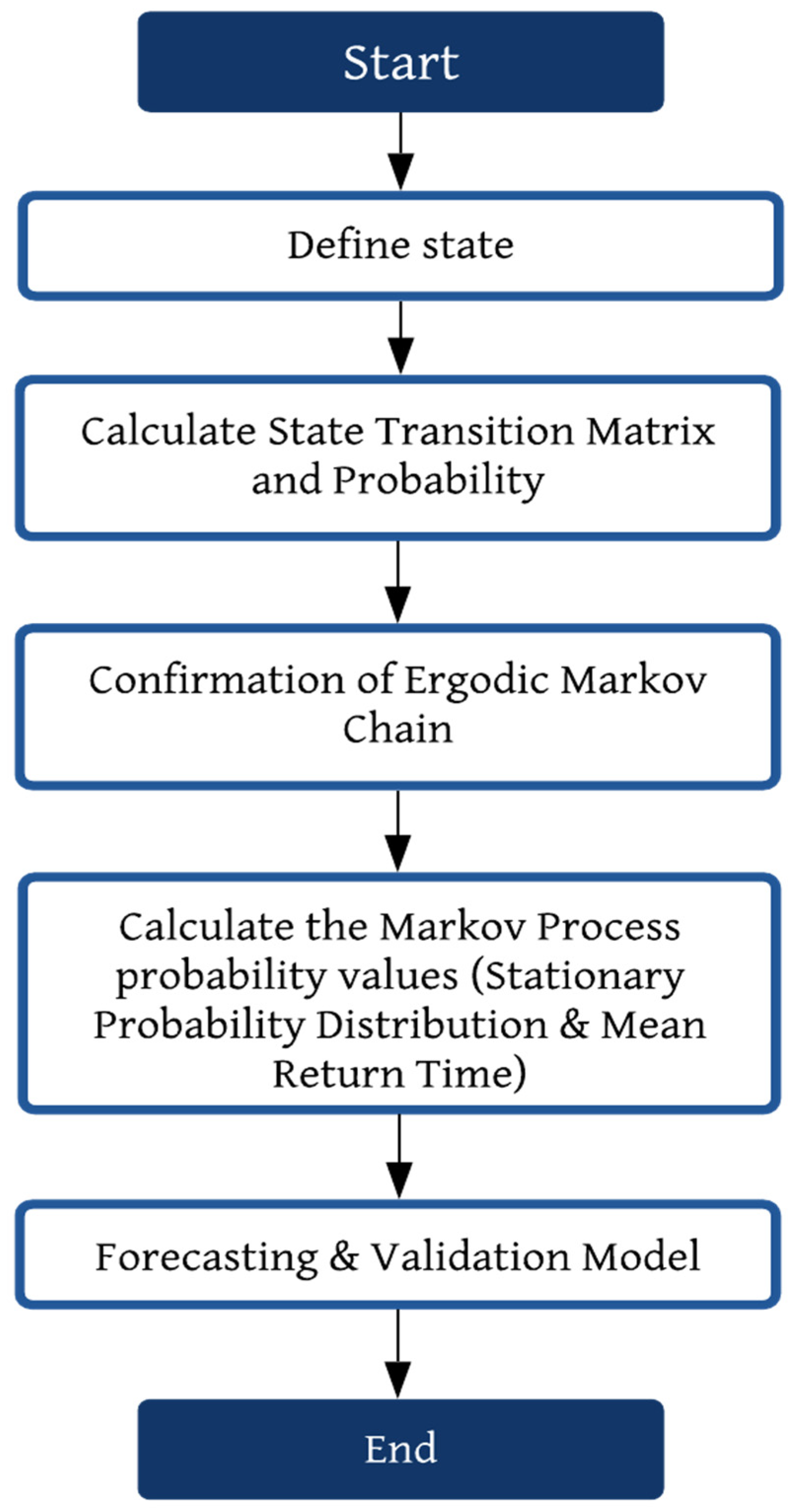
The Markov chain technique is adopted in this study. The proposed method is a stochastic process by introducing the simplest way of statistical dependence. In addition, the future behavior of this process is not concerned with the past behavior. To highlight the structure of the proposed Markov chain method, the framework is visualized in Figure 1.

The algorithms of the proposed Markov chain method consisted of five steps as shown below.

Step 1. Define state for the Markov chain process.

In this step, states or thresholds must be determined for the Markov chain process based on the data that were used in the development of the model.

Step 2. Construct the state transition matrix, N, and state transition probability, P.

State transition matrix, N, as defined by the Markov chain, indicates the observed frequency of transition or jump from one state to another state. Thus,

$$N=\left[\begin{array}{ccc}{n}_{11}& \cdots & n_{1s}\\ ⋮& \ddots & ⋮\\ n_{s1}& \cdots & n_{ss}\end{array}\right],$$

(2)

where $n_{ij}$ is the number of transitions in a sequence for state i followed by state j. Let P be a transition matrix or stochastic matrix that describes all the transition probabilities for each state of the Markov chain model. Hence, P is denoted as below;

$$P=\left[\begin{array}{ccc}{p}_{11}& \cdots & p_{1s}\\ ⋮& \ddots & ⋮\\ p_{s1}& \cdots & p_{ss}\end{array}\right], i,j\in I,$$

(3)

then,

$$P\left\{X_{t+1}=j|X_t=i\right\}=p_{ij}.$$

(4)

This term is for one-step probability. For transition probabilities that are independent with time t, it indicates as homogenous or stationary Markov chain. Hence,

$$P\left\{X_{t+1}=j|X_t=i\right\}=P\left\{X_1=j|X_0=i\right\}=p_{ij}.$$

(5)

The matrix P insists non-negative elements with row sum unity. Thus,

$$0\le p_{ij}\le 1\mathrm{and}{{\displaystyle \sum }}_{j=1}^t{p}_{ij}=1, \sqrt{i}\in I .$$

(6)

The probability

$$p_{ij}\left(k\right)=P\left\{X_{n+k}=j|X_n=i\right\}, \sqrt{k}>0,n\ge 0, i,j\in I$$

(7)

is the k-step transition probability from state i to state j in k steps. The transition matrix P has the following property.

$$P\left(n\right)=P^{n-1}\times P=P^n$$

(8)

Step 3. Confirmation of ergodic Markov chain.

The confirmation of an ergodic Markov chain must be made to identify the existence of limiting distribution in this chain by classifying the state of P. It can be divided into three sections; irreducible Markov chain, periodicity Markov chain, and recurrent and transient states [25,26,27].

1. Irreducible Markov Chain

State i is reachable from state j if $p_{ij}^{\left(n\right)}=0$ for some $n\ge 0$. Both states are accessible and can be said as communicate, $i\leftrightarrow j$. The properties for the communicate relation [7]:

• State i communicates with state i, for all $i\ge 0$;
• If state i communicates with state j, then state j communicates with state i;
• If state i communicates with state j, then state j communicates with state k, then state i communicates with state k.

When the two states communicate in the same class, the Markov chain can be concluded as irreducible if there is only one class.

2. Periodicity Markov Chain

State i has period d if $p_{ii}^{\left(n\right)}=0$ when n is not divisible by d and d is the largest integer. For a Markov chain that has period one for each state called as aperiodic.

3. Recurrent and Transient States

In the Markov chain, for any state i, let $f_i$ be the probability that is starting in state i, the process will ever re-enter state i. State i can be conclude as recurrent if $f_i=1$ and transient if $f_i<1$ [9]. For a finite Markov chain, state i is recurrent if and only if

$${{\displaystyle \sum }}_{n=1}^{\infty }{P}_{ii}^{\left(n\right)}=\infty .$$

(9)

For starting in state i, the expected time until the process returns to itself is finite if the state i is recurrent. It can be shown that all recurrent states are positive recurrent. For positive recurrent and aperiodic states can be conclude as ergodic [25].

Step 4. Markov process probability values.

For this step, stationary probability distribution and mean return time can be obtained for Markov process probability values. Stationary probability distribution will describe the behavior of air pollution in long term forecasting where the chain is sufficient for a long period of time with steady-state probabilities that are independent from initial conditions [27]. For an ergodic Markov chain, the limiting distribution existed for stationary probability distribution and can be represent as

$${\pi }_j=\underset{n\to \infty }{\lim }P\left(X_n=j|X_0=i\right).$$

(10)

Then, $P_j\left(n\right)={{\displaystyle \sum }}_k{P}_k\left(n-1\right)P_{kj}$ becomes ${\pi }_j={{\displaystyle \sum }}_k{\pi }_k{P}_{kj}$, as $n\to \infty$ for $j=0,1,2,\dots$. Hence, the probability of finding the process in state j is irrespective of starting state for a long duration in the process [25]. The value of ${\pi }_j$ will be high if the probability occurrences of state j is high [26]. Prediction in the long run behavior also has pitfalls and disadvantages in various problems such as lacking information and accumulated errors [28].

Furthermore, mean return time needs to be calculated to identify the average time for specific states to return back to itself, $m_j$. It can be denoted as

$$m_{ij}=\frac{1}{{\pi }_j}.$$

(11)

Step 5. Forecasting and model validation.

Forecasting value can be obtained from the initial probability and state transition probability through Equation (12).

$$P\left(S_j\right)={{\displaystyle \sum }}_{i=1}^{n}P\left(S_i\right)P_{ij},$$

(12)

where $P\left(S_i\right)$ is an initial probability and $P_{ij}$ is a state transition probability.

For model validation, Chi-square test is used to check the validity of the Markov chain based on the independence assumption [11]. The null hypothesis is the selected data on consecutive time is independent while the alternative hypothesis is the selected data on consecutive time is dependent.

$$X_{calculated}^2={\displaystyle \sum }\frac{{\left(Observed-Expected\right)}^2}{Expected}$$

(13)

The null hypothesis is rejected when $X_{calculated}^2$ is greater than $X_{tabulated}^2$ on the 0.05 critical regions [11].

4. Case Study

In this section, a case study is presented to verify the developed Markov chain model in forecasting air quality.

4.1. Background of the Problem

This study focuses on the haze problem in the Malaysian region of Sarawak. We specifically focus on the northern part, Miri. Miri is a coastal city that is located near the border of Brunei Darussalam. The study area covers 997.43 km², 798 km northeast of Kuching and 329 km southwest of Kota Kinabalu. The study area is the second largest city in Sarawak with a population of 358,020 people as of 2016 [29]. Last year, in 2018, there was a serious occurrence of haze due to the forest fires and open burnings in the late evening and at night, and the reading soared to 228 (very unhealthy state) [30].

4.2. Data Collection and API States

The five-year data from 2013 until 2017 were collected from the Department of Environment (DOE) based on hourly data. Hourly API was derived based on data retrieved from Continuous Air Quality Monitoring (CAQM) stations throughout the country. In Malaysia, there are 65 monitoring stations that can detect the changes in air quality status [15]. API is the indicator for status of air quality at any particular area. It can be calculated based on the average air pollutants concentrations; SO₂, NO₂, CO, O₃, PM_2.5, and PM₁₀ and the value can be determined based on the dominant pollutant. API readings can be obtained after complete one-hour cycle for data retrieval processes [31].

Table 1. Air Pollution Index (API) and health implications by Malaysia’s Department of Environment [33].

State	API	Air Quality Status	Health Implications
1	0–50	Good	Low pollution without any bad effect on health
2	51–100	Moderate	Moderate pollution that does not pose any bad effect on health
3	101–200	Unhealthy	Worsen the health condition of high-risk people. High-risk people = people with heart and lung complications
4	201–300	Very Unhealthy	Worsen the health condition and low tolerance of physical exercises to people with heart and lung complications. Affect public health
5	>300	Hazardous	Hazardous to high-risk people and public health

shows the scale and terms for API that were used in describing the level of air quality [32].

4.3. The Analysis of Data Using the Proposed Markov Chain Method

Table 2. Frequency of API state categories in Miri, Sarawak.

State	Status of API	Frequency
1	Good	18,194
2	Moderate	24,368
3	Unhealthy	1141
4	Very Unhealthy	58
5	Hazardous	63

lists the frequencies of each category (API states) for the five years of the categorical time series. The highest frequency was on moderate state while the lowest was on very unhealthy state with a frequency of 58.

As shown in Table 2, the frequency of a hazardous API status is still below 100, which is a frequency of 63 for over five years in Miri. Meanwhile,

Table 3. State transition matrix in Miri, Sarawak.

Present State	Future State
	Good (1)	Moderate (2)	Unhealthy (3)	Very Unhealthy (4)	Hazardous (5)
Good (1)	40,371	80	0	0	0
Moderate (2)	80	3078	8	0	0
Unhealthy (3)	0	8	154	1	0
Very Unhealthy (4)	0	0	1	3	1
Hazardous (5)	0	0	0	1	37

shows the observed frequency of transition for API in Miri based on Equation (2).

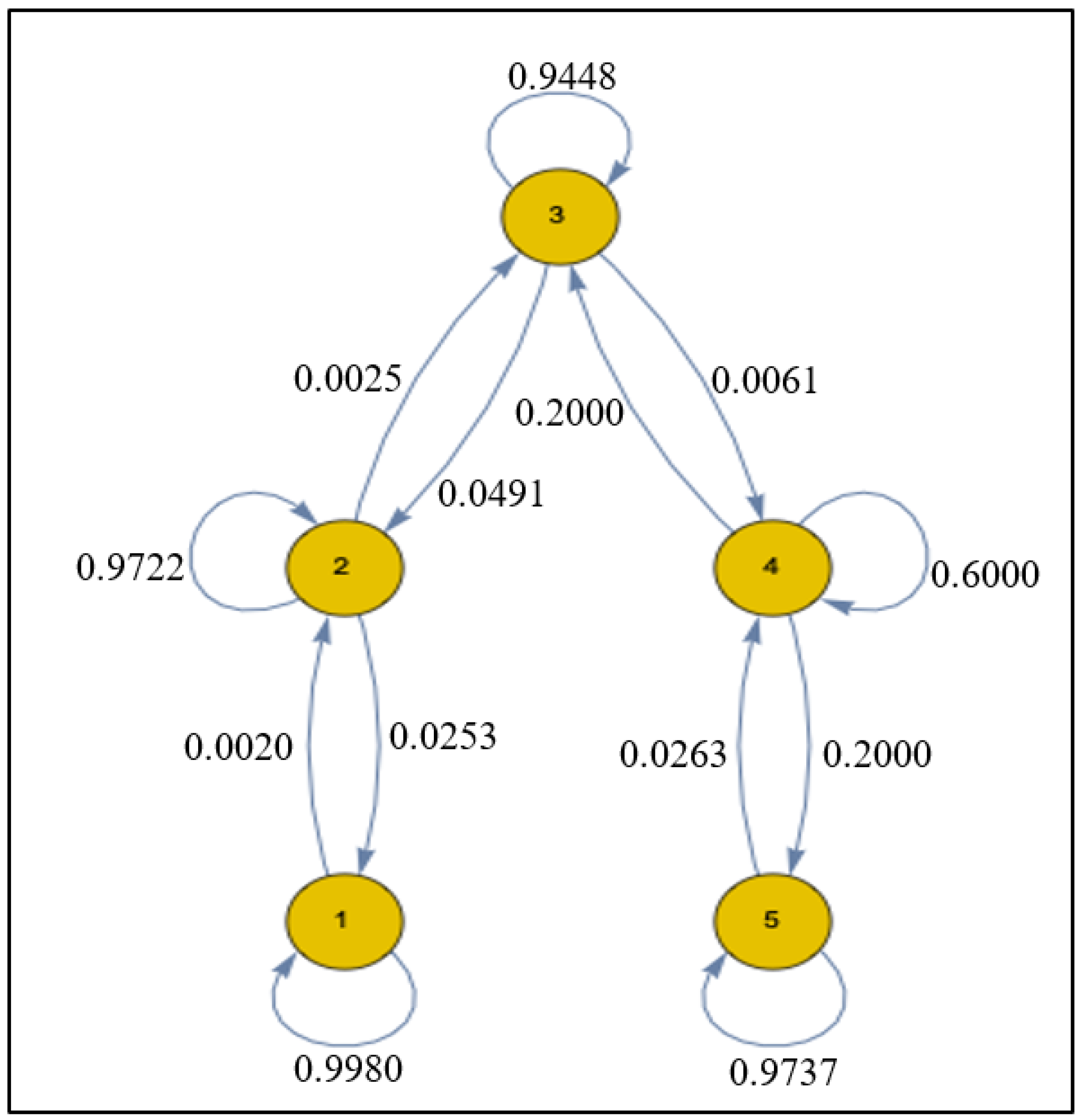
The close observations of API over the study period show that it involves five different states of transition. The transition probability can provide an idea about the occurrence of the future state likelihood followed by the decision making. The API of 43,823th hours shows that the frequency for a good state was 40,451th hours, for moderate and unhealthy both 3166 and 163 h. Then, followed by very unhealthy and hazardous state 5 and 38 h. The transition probability of $P_{API}$ by using Equation (3) provides the information regarding the behavior of air quality transit from one state to another state and can be constructed as shown below.

$$P_{API}=\left[\begin{array}{ccccc}0.9980& 0.0020& 0.0000& 0.0000& 0.0000\\ 0.0253& 0.9722& 0.0025& 0.0000& 0.0000\\ 0.0000& 0.0491& 0.9448& 0.0061& 0.0000\\ 0.0000& 0.0000& 0.2000& 0.6000& 0.2000\\ 0.0000& 0.0000& 0.0000& 0.0263& 0.9737\end{array}\right]$$

(14)

The transition diagram for the state transition probability chain of API is shown in Figure 2.

Therefore, based on step 3 mentioned before, the findings show that the developed Markov chain model was irreducible, aperiodic, and recurrent. Thus, it can confirm that the model is an ergodic Markov chain.

4.4. Markov Process Probability Values

For forecasting in long run behavior, the probability of the states will be referred to the stationary probability distribution value. The value below derived the steady state probability of API in the future by using Equation (10) for the five different states.

$${\pi }_j=\left[\begin{array}{ccccc}0.9231& 0.0722& 0.0037& 0.0001& 0.0009\end{array}\right]$$

(15)

${\pi }_j$ indicates that the good state of equilibrium is 0.9231, moderate is 0.0722, unhealthy is 0.0037 followed by very unhealthy and hazardous, 0.0001 and 0.0009. Therefore, the risk of haze to occur in the future is low based on the lowest proportion in very unhealthy and hazardous state above. For mean return time, the average time for the state stays in the same state and can be obtained based on Equation (11). Stationary probability distribution was used in order to determine the mean return time for every state of API as shown in the matrix below.

$$m_j=\left[\begin{array}{ccccc}1.0834& 13.8418& 268.8528& 8764.6000& 1153.2368\end{array}\right]$$

(16)

The results show that mean return time for good state staying in the same state is 1 h and moderate state is on average 14 h. For unhealthy state, the average time that API should visit the state is 11 days (269 h). However, for the very unhealthy and hazardous state, it will take on average 365 days (8765 h) and 48 days (1153 h) for the API in Miri.

4.5. Forecasting and Model Validation

Based on Equation (12), the next probability can be obtained by multiplying the initial state vector and state transition probability. The initial state vector for API at the end of 43,823th hours is good state so it will be $\left(1.0000,0.0000,0.0000,0.0000,0.0000\right)$.

$$\begin{gathered} \eta \left(43824\right)=\eta \left(43823\right)\times P_{API} \\ =\left[\begin{array}{ccccc}1.0000& 0.0000& 0.0000& 0.0000& 0.0000\end{array}\right]\left[\begin{array}{ccccc}0.9980& 0.0020& 0.000& 0.000& 0.000\\ 0.0253& 0.9722& 0.0025& 0.000& 0.000\\ 0.0000& 0.0491& 0.9448& 0.0061& 0.000\\ 0.0000& 0.0000& 0.2000& 0.6000& 0.2000\\ 0.0000& 0.0000& 0.000& 0.0263& 0.9737\end{array}\right] \\ =\left[\begin{array}{ccccc}0.9980& 0.0020& 0.0000& 0.0000& 0.0000\end{array}\right] \end{gathered}$$

(17)

The above probability shows that the API for the good state is 0.9980 and 0.0020 for the moderate state at the end of the 43,824th hours. However, haze will not occur because of the zero probability for the unhealthy, very unhealthy, and hazardous state on that particular hour. Following a similar manner, the probability for API at 43,825th hours is shown below.

$$\begin{gathered} \eta \left(43825\right)=\eta \left(43824\right)\times P_{API} \\ =\left[\begin{array}{ccccc}0.9980& 0.0020& 0.0000& 0.0000& 0.0000\end{array}\right]\left[\begin{array}{ccccc}0.9980& 0.0020& 0.0000& 0.0000& 0.0000\\ 0.0253& 0.9722& 0.0025& 0.0000& 0.0000\\ 0.0000& 0.0491& 0.9448& 0.0061& 0.0000\\ 0.0000& 0.0000& 0.2000& 0.6000& 0.2000\\ 0.0000& 0.0000& 0.0000& 0.0263& 0.9737\end{array}\right] \\ =\left[\begin{array}{ccccc}0.9961& 0.0020& 0.0000& 0.0000& 0.0000\end{array}\right] \end{gathered}$$

(18)

The suitability for the data with the method has been checked based on the hypothesis testing to validate the appropriateness of the developed model. The null hypothesis is the API on consecutive hours is independent while the alternative hypothesis is the API on consecutive hours is dependent. Based on

Table 4. Statistical results of API data.

Test Perform	Calculated Value	Chi Square Table Value on 0.05 Critical Region
Goodness of fit test (X2)	2667.7357	26.2962

, the calculated value is 2667.7357 and is greater than the significance value on the region 0.05 with 16 degrees of freedom, 26.2962. If the calculated value is greater than the tabulated value, the hypothesis is rejected. The results indicate that the API of a current hour is dependent on the preceding hour. Thus, it will validate the dependency assumption.

4.6. Performance of the Developed Model

The performance of the model can be seen based on the smallest value of error by calculating the error value between actual and forecasting data [34]. Types of error measurement that were used in this study are root mean square error (RMSE) and mean absolute percentage error (MAPE). The results in

Table 5. Model comparison of forecast values.

Model	RMSE	MAPE
Markov chain	0.5330	0.1979%
SARIMA	31.4955	0.7338%

showed that the Markov chain model has the smallest value which is 0.5330 for RMSE and 0.1979% for MAPE compared to the SARIMA model [35].

5. Discussion

The results of this study have demonstrated how the Markov chain forecasting model fits the data, and also, how it is able to predict future API behavior. This developed model also generates results which are more reliable than comparable models, due to its capability of random walk in transition matrix and memoryless property. This viewpoint is also consisted with the earlier findings of Piccardi et al. [36], Hazra et al. [37], and Tserenjigmid [38]. Collectively, this study outlines a critical role in developing a model that provides a comprehensive yet simple prediction, which can help solve complicated forecasting problems. Furthermore, it also provides important insights on how to improve air quality forecasting problems. Hence, the analysis results indicate that it is easily understood by decision makers and can be computed easily using modest computation. For future research, it is recommended to use higher order Markov chains to gain better insight in forecasting into the behavior of air pollution.

6. Conclusions

In this paper, a Markov chain method has been successfully developed. The developed model in predicting future behavior of API assumes that the performance of API is completely affected by the stochastic factors. The model was comparable and performed better in terms of mean return time for the state of API in a period of time. A case study of the air pollution problem in the northern part of Sarawak, Miri, during the period of January 2013 to December 2017 which has five finite states was implemented using the Markov chain to get the future behavior of API. The predicted results were obtained in terms of probability of the state in API. Therefore, it does not provide the actual value of API for the forecasting results.

Based on the results of transition probability, it can be said that if the level of air pollution in the previous period was in the good state, then the occurrence probability of the good state in the next period (0.9980) will be higher than the other state (0.0020). At the same time, if the previous period of API was in hazardous state, the likelihood of hazardous state in the next period will be higher (0.9737) than the other four states of API (0.0263). The probability of the good state in the long run behavior of API is larger (0.9231) than the other state which is 0.0722 and 0.0037 for moderate and unhealthy state. Meanwhile, for the very unhealthy and hazardous state the lowest proportion is 0.0001 and 0.0009. Thus, we can conclude that the risk of haze to occur is low. Lastly, based on the performance evaluation, the Markov chain model is more appropriate and successful as a forecasting tool for API which is 0.5330 for RMSE and 0.1979% for MAPE. The analysis and findings of this study can be used in decision making and as a prevention plan for DOE during hazy weather.

References

- Elgharbi, S.; Esghir, M.; Ibrihich, O.; Abarda, A.; El Hajji, S.; Elbernoussi, S. Grey-Markov Model for the Prediction of the Electricity Production and Consumption. In Lecture Notes in Networks and Systems; Springer New York: New York, NY, USA, 2020; Volume 81, pp. 206–219. [Google Scholar]
- Winston, W.L.; Goldberg, J.B. Operations Research: Applications and Algorithms; Thomson Brooks/Cole: Belmont, CA, USA, 2004. [Google Scholar]
- Seneta, E. Andrei Andreevich Markov. In Statisticians of the Centuries; Heyde, C.C., Seneta, E., Crépel, P., Fienberg, S.E., Gani, J., Eds.; Springer New York: New York, NY, USA, 2001; pp. 243–247. [Google Scholar]
- Chatfield, C. Statistical Inference Regarding Markov Chain Models. J. R. Stat. Society. Ser. C (Appl. Stat.) 1973, 22, 7–20. [Google Scholar] [CrossRef]
- Ibarra-Berastegi, G.; Elias, A.; Barona, A.; Saenz, J.; Ezcurra, A.; Diaz de Argandoña, J. From diagnosis to prognosis for forecasting air pollution using neural networks: Air pollution monitoring in Bilbao. Environ. Model. Softw. 2008, 23, 622–637. [Google Scholar] [CrossRef]
- Yan Chan, K.; Jian, L. Identification of significant factors for air pollution levels using a neural network based knowledge discovery system. Neurocomputing 2013, 99, 564–569. [Google Scholar] [CrossRef] [Green Version]
- Fernando, H.J.S.; Mammarella, M.C.; Grandoni, G.; Fedele, P.; Di Marco, R.; Dimitrova, R.; Hyde, P. Forecasting PM10 in metropolitan areas: Efficacy of neural networks. Environ. Pollut. 2012, 163, 62–67. [Google Scholar] [CrossRef] [PubMed]
- Güler, N.; Güneri İşçi, Ö. The regional prediction model of PM10 concentrations for Turkey. Atmos. Res. 2016, 180, 64–77. [Google Scholar]
- Ong, B.T.; Sugiura, K.; Zettsu, K. Dynamically pre-trained deep recurrent neural networks using environmental monitoring data for predicting PM2.5. Neural Comput. Appl. 2016, 27, 1553–1566. [Google Scholar] [CrossRef] [PubMed]
- Saad, S.A.; Adnan, F.A.; Ibrahim, H.; Rahim, R. Manpower planning using Markov Chain model. Aip Conf. Proc. 2014, 1605, 1123–1127. [Google Scholar]
- Zhou, Y.; Wang, L.; Zhong, R.; Tan, Y. A Markov Chain Based Demand Prediction Model for Stations in Bike Sharing Systems. Math. Probl. Eng. 2018, 1–8. [Google Scholar] [CrossRef]
- Chung, Y.-S. A Study of the Prediction of Crime to Time Variation using Markov Chain. J. Adv. Inf. Technol. Converg. 2011, 1. [Google Scholar] [CrossRef]
- Choji, D.N.; Kassem, S.N.E.G.T. Markov Chain Model Application on Share Price Movement in Stock Market. Comput. Eng. Intell. Syst. 2013, 4, 84–95. [Google Scholar]
- Masseran, N. Markov Chain model for the stochastic behaviors of wind-direction data. Energy Convers. Manag. 2015, 92, 266–274. [Google Scholar] [CrossRef]
- DOE Chronology of Haze Episodes in Malaysia. Available online: https://www.doe.gov.my/portalv1/en/info-umum/info-kualiti-udara/kronologi-episod-jerebu-di-malaysia/319123 (accessed on 23 March 2019).
- Suhaimi, N.; Ghazali, N.A.; Nasir, M.Y.; Mokhtar, M.I.Z.; Ramli, N.A. Markov Chain Monte Carlo method for handling missing data in air quality datasets. Malays. J. Anal. Sci. 2017, 21, 552–559. [Google Scholar]
- Luis, H.-R.; Lara, P.; Ortiz, E.; López Bracho, R.; Gonzalez-Trejo, J. Evaluation of air pollution control policies in Mexico City using finite Markov chain observation model. Rev. De Matemática 2010, 16, 255. [Google Scholar]
- Luo, L.; Zhang, F.; Zhang, W.; Sun, L.; Li, C.; Huang, D.; Han, G.; Wang, B. Markov Chain-Based Acute Effect Estimation of Air Pollution on Elder Asthma Hospitalization. J. Healthc. Eng. 2017, 2017, 2463065. [Google Scholar] [CrossRef] [PubMed]
- Candelieri, A.; Archetti, F.; Giordani, I.; Arosio, G. Markov-Based Approaches to Support Policies Makers in Environment and Healthcare; International Congress on Environmental Modelling and Software Managing Resources of a Limited Planet, Sixth Biennial Meeting: Leipzig, Germany, 2012. [Google Scholar]
- Gómez-Losada, Á. Clustering Air Monitoring Stations According to Background and Ambient Pollution Using Hidden Markov Models and Multidimensional Scaling; Data Science, Cham, 2017//, 2017; Palumbo, F., Montanari, A., Vichi, M., Eds.; Springer International Publishing: Cham, Switzerland, 2017; pp. 123–132. [Google Scholar]
- Nebenzal, A.; Fishbain, B. Long-Term Forecasting of Nitrogen Dioxide Ambient Levels in Metropolitan Areas Using the Discrete-Time Markov Model. Environ. Model. Softw. 2018, 107, 175–185. [Google Scholar] [CrossRef]
- Nicas, M. Markov Modeling of Contaminant Concentrations in Indoor Air. Aihaj A J. Sci. Occup. Environ. Health Saf. 2000, 61, 484–491. [Google Scholar]
- Billingsley, P. Statistical Methods in Markov Chains. Ann. Math. Statist. 1961, 32, 12–40. [Google Scholar] [CrossRef]
- Lawler, G.F. Introduction to Stochastic Processes; CRC Press: London, UK; New York, NY, USA, 2006. [Google Scholar]
- Pinsky, M.A.; Karlin, S. The Long Run Behavior of Markov Chains. In An Introduction to Stochastic Modeling, 4th ed.; Pinsky, M.A., Karlin, S., Eds.; Academic Press: Boston, MA, USA, 2011; pp. 165–222. [Google Scholar]
- Grinstead, C.; Snell, L. Grinstead and Snell’s Introduction to Probability; American Mathematical Society: Providence, RI, USA, 2006. [Google Scholar]
- Ibe, O.C. 4—Discrete-Time Markov Chains. In Markov Processes for Stochastic Modeling, 2nd ed.; Elsevier: Oxford, UK, 2013; pp. 59–84. [Google Scholar]
- Chatfield, C.; Weigend, A.S. Time series prediction: Forecasting the future and understanding the past: Neil A. Gershenfeld and Andreas S. Weigend, 1994, ’The future of time series’, in: A.S. Weigend and N.A. Gershenfeld, eds., (Addison-Wesley, Reading, MA), 1–70. Int. J. Forecast. 1994, 10, 161–163. [Google Scholar] [CrossRef]
- JUPEM. Atlas kebangsaan Malaysia; Jabatan Ukur dan Pemetaan Malaysia: Kuala Lumpur, Malaysia, 2016. [Google Scholar]
- Sidi, K. Forest Fires, Haze in Sarawak due to Weak Enforcement. Available online: https://www.nst.com.my/news/nation/2019/05/488281/forest-fires-haze-sarawak-due-weak-enforcement (accessed on 14 May 2019).
- DOE Air Quality. Available online: https://www.doe.gov.my/portalv1/en/info-umum/kuality-udara/114 (accessed on 10 April 2019).
- DOE Air Pollution Index of Malaysia. Available online: http://apims.doe.gov.my (accessed on 1 March 2019).
- DOE Air Quality Standards. Available online: https://www.doe.gov.my/portalv1/en/info-umum/english-air-quality-trend/108 (accessed on 31 March 2019).
- Bowerman, B.L.; O’Connell, R.T.; Koehler, A.B. Forecasting, Time Series, and Regression: An Applied Approach; Thomson Brooks/Cole: Belmont, CA, USA, 2005. [Google Scholar]
- Lee, M.H.; Rahman, N.; Suhartono, S.; Latif, M.T.; Nor, M.; Kamisan, N. Seasonal ARIMA for forecasting air pollution index: A case study. Am. J. Appl. Sci. 2012, 9, 570–578. [Google Scholar]
- Piccardi, C.; Riccaboni, M.; Tajoli, L.; Zhu, Z. Random walks on the world input–output network. J. Complex Netw. 2017, 6, 187–205. [Google Scholar] [CrossRef]
- Hazra, T.; Nene, M.J.; Kumar, C.R.S. A Strategic Framework for Searching Mobile Targets Using Mobile Sensors. Wirel. Pers. Commun. 2017, 95, 1–16. [Google Scholar] [CrossRef]
- Tserenjigmid, G. On the characterization of linear habit formation. Econ. Theory 2019, 1–45. Available online: https://doi.org/10.1007/s00199-019-01202-x (accessed on 15 September 2019). [CrossRef]
Figure 1.
Framework of the proposed Markov chain method.
Figure 2.
Chain of transition probability for API in Miri.