Spatially Explicit Assessment of Social Vulnerability in Coastal China

Abstract

Social vulnerability assessment has been recognized as a reliable and effective measure for informing coastal hazard management. Although significant advances have been made in the study of social vulnerability for over two decades, China’s social vulnerability profiles are mainly based on administrative unit. Consequently, no detailed distribution is provided, and the capability to diagnose human risks is hindered. In this study, we established a social vulnerability index (SoVI) in 2000 and 2010 at a spatial resolution of 250 m for China’s coastal zone by combining the potential exposure index (PEI) and social resilience index (SRI). The PEI with a 250 m resolution was obtained by fitting the census data and multisource remote sensing data in random forest model. The county-level SRI was evaluated through principal component analysis based on 33 socioeconomic variables. For identifying the spatiotemporal change, we used global and local Moran’s I to map clusters of SoVI and its percent change in the decade. The results suggest the following: (1) Counties in the Yangtze River Delta, Pearl River Delta, and eastern Guangzhou, except several small hot spots, exhibited the most vulnerability, especially in urban areas, whereas those in Hainan and southern Liaoning presented the least vulnerability. (2) Notable increases were emphasized in Tianjin, Yangtze River Delta, and Pearl River Delta. The spatiotemporal variation and heterogeneity in social vulnerability obtained through this analysis will provide a scientific basis to decision-makers to focus risk mitigation effort.

1. Introduction

The population density in coastal zones is significantly higher than other areas [1,2] due to sufficient resources for human activities and civilization of early days [3]. For example, maritime transport connects the whole world, and the port is an important part. Most of the world-class urban agglomerations are located in coastal zones, such as the Atlantic coast of the northeastern United States, the Pacific coast of Japan, the urban clusters of northwestern Europe, and the Yangtze River Delta of China. The coastal migration trend will continue [4] as a consequence of accelerating development and utilization [5]. Approximately 50% of the population is predicted to settle in the coastal areas by 2030 [6], thus, they are not only the precious land resources of coastal countries, but also the link of foreign trade and cultural exchange. Coastal areas are highly productive at a global scale and occupy an important position in the ecosystem. For example, coastal wetlands provide numerous important functions, such as waste assimilation, nursery areas for fisheries and mariculture, flood protection, and nature conservation [7]. However, coasts are easily subjected to natural hazards such as tropical cyclones, terrestrial floods, storm surges, and tsunamis. [8,9]. Most coastal zones worldwide are affected by climate change, especially global sea level rise [10,11], which influences the frequency and intensity of storm surge [12]. China’s coast has played an important role in various aspects, namely, economic, political, and military [13]. Considering the high concentration of assets and population, the vulnerability of China’s coastal zones should be evaluated, which is now regarded as a requirement for the effective development of emergency management capability [14].

In 1974, White [15] first defined vulnerability as “the degree to which a system, sub-system, or component which is likely to experience harm due to exposure to a hazard, either a perturbation or stress”. Thereafter, vulnerability has been one of the conceptually written terms rooting in geography and natural hazard research [16], which now relates to multiple natural impacts and social effects, such as salinity incursion, drought, bushfire, flooding and inundation, erosion and sedimentation, poverty, and land use change [3,17,18,19]. Vulnerability has been differently conceptualized and represented among different studies because of the various social contexts and stress effects [20,21,22,23,24]. With regard to environmental hazards, numerous researchers distinguish biophysical and social vulnerabilities as two dimensions [3,25,26,27,28,29,30,31,32,33,34].

Biophysical vulnerability focuses on hazards’ magnitude and duration, topography and land cover that influence the potential for harm [23,35,36]. Such vulnerability arises from the approach based on assessments of hazardous events and their effects; the role of human systems in mediating the risk is downplayed or neglected [37].

On the contrary, social vulnerability constructs on human community attributes, such as living standards, economic status, public infrastructure, institution and demographics, and historical process [38,39,40,41,42]. These factors influence the society’s capability to prepare for, respond to, and recover from natural disasters [3,43,44].

Social vulnerability is a pre-event state of being [25,45], indicating the sensitivity and susceptibility of a system to natural hazards. Such vulnerability is more complex than the biophysical one. However, socially created vulnerability can be reduced through policy implementation and human activities, thereby attracting an increasing number of researchers. In China, Chen et al. [46] measured social vulnerability to natural hazards in the Yangtze River Delta region. Ge et al. and Su et al. [47,48] categorized social vulnerability patterns in China’s coastal zone. Zhou et al. [49] indicated the spatiotemporal change of social vulnerability in China from 1980 to 2010. However, nearly all social vulnerability assessments are based on administrative boundaries and are inaccurate because the actual distribution is fairly heterogeneous across these spatial units. In the present work, we refer to the model proposed by Cutter et al. [29], which shows that social vulnerability consists of two parts: potential exposure (PE) and social resilience (SR) [50,51]. The final explicit raster-level social vulnerability index (SoVI) [47,52] can be obtained by combining the potential exposure index (PEI) of 250 m resolution with the county-level social resilience index (SRI). Accordingly, the spatial delineation of social vulnerability is significantly improved and hotspots of high social vulnerability can be identified within administrative units.

“Potential exposure” can be understood as the degree to which a system will be adversely affected by natural hazards. Although all people living in hazardous areas are vulnerable [14], we use the spatial distribution of population as the index for PE [3,53,54,55]. Given the same degree of exposure to hazards, regions with several inhabitants will be more socially vulnerable than those with low densities [53]. Thus, precise population distribution is crucial in PE mapping. In China, census data are accurate first-hand statistics that can be used to explore population distribution and have been adopted by most studies [46,47,48]. However, census data provide no detailed information because people are nonuniformly distributed within administrative boundaries but gather in the city center [55,56]. The emergence of remote sensing and geographical information system (GIS) techniques provides us with a new way to obtain explicit population distribution data [56,57]. We combined multi-source remote sensing data (GHSL, NDVI, NTL, land use and DEM) in the random forest (RF) model to disaggregate the county-level census data to 250 × 250 m grids [58,59]. As such, accurate population maps were produced, which is conducive to the PE assessment.

Resilience reveals the capability of a social system to resist and recover from a disturbance within the normal confines of daily life [60,61]. Thus, the more resilient a society is, the less vulnerable it will be [62]. This study regards counties as the evaluation units for the following reasons: (1) the most accurate socioeconomic data that we can obtain are those at the county level and (2) disaster management and recovery measures are implemented at the county level [49]. Considering that SR is related to multiple socioeconomic characteristics, a large amount of measurable variables were aggregated using principal component analysis (PCA) to establish the SRI. This method was advocated by Cutter et al. in 2003 [29] and became the primary procedure in social vulnerability research.

Most recent studies on the vulnerability of China’s society are concentrated in a certain year, ignoring its development trend over time. On this basis, the present work addressed the last critique of social vulnerability assessment by providing a time series of changes in vulnerability patterns. The dynamic nature of social vulnerability is illustrated by using a replication of the baseline indicators for China’s coastal zone over two different time periods (2000 and 2010). We used the global Moran’s I spatial autocorrelation tool in ArcGIS 10.2 to test for significant clustering in SoVI for 2000 and 2010. Subsequently, the local indicators of spatial association (LISA) cluster map based on local Moran’s I was used to explore the distribution of hot and cold spots [49,60,63]. Then, the percent change of SoVI was calculated, and local Moran’s I was used to identify regions with high temporal change [64].

In this study, we focused on China’s coastal zone as a case study. This study aimed to improve SoVI spatial delineation and investigate the SoVI spatiotemporal change from 2000 to 2010. The research contents are as follows: (1) construction of PEI and SRI distribution maps, (2) aggregation of PEI and SRI to obtain SoVI and calculation of the percent change, and (3) use of global and local Moran’s I to identify a local cluster on the basis of the abovementioned results for locating the areas with SoVI spatiotemporal change.

2. Study Area

The study area (Figure 1) consisted of 292 county-level units, including counties, county-level cities, and city districts, which are in the third level of Chinese administrative hierarchy [48]. Hong Kong, Macao, and Taiwan were excluded because of their distinct political and economic environment. Mainland China, which geographically extends from 108°20′59″ E to 124°20′56″ E and from 18°15′16″ N to 39°59′56″ N, has a coastline of over 18,000 km crossing three climate zones: tropical, sub-tropical, and temperate [47]. The coastal zone scope is a long narrow belt area alongshore, stretching from the Liaodong Bay in the north to the Gulf of Tonkin in the south [47]. With the Hangzhou Bay as the boundary, the northern coastal zone is dominated by the plain coast (sand shore), whereas the southern part is dominated by the mountain coast (rock bank) [13]. The coastal zone is easily attacked by natural hazards, such as storm surge, tsunami, and earthquake, because of its complex climatic and geological conditions. For example, 345 tropical cyclones hit the Chinese coastal zone between 1961 and 2008 [65], posing a great threat to the safety of people’s lives and property. China Statistical Yearbook 2011 indicates that the coastal region contributes approximately 18% of the total population and 35% of the national GDP compared with nearly 4% occupation of land area [47,48]. The developed but highly vulnerable area can be effectively managed on the basis of the social vulnerability measurement to combat natural disaster risks, which was the purpose of this case study.

3. Materials and Method

3.1. Data Source

(1)

Demographic and socioeconomic data: The administrative division of China consists of five practical levels: province (Admin. Level 1), prefecture (Admin. Level 2), county (Admin. Level 3), township (Admin. Level 4), and village (Admin. Level 5). To fit the RF model, the census data at the county level (Admin. Level 3) for the coastal zone were obtained from China’s fifth (2000) and sixth (2010) National Census. The census data at the 2010 township level (Admin. Level 4) were used to evaluate the accuracy of the simulated population map (the township-level census data for 2000 were unavailable). Other demographic and socioeconomic data for SRI estimation were derived from the National Census, statistical yearbooks of coastal provinces and municipalities (Liaoning, Hebei, Tianjin, Shandong, Jiangsu, Shanghai, Zhejiang, Fujian, Guangdong, Guangxi, and Hainan), China Urban Statistical Yearbook 2001, and China Regional Economic Statistical Yearbook 2011.

(2)

NTL imagery: The stable 2000 and 2010 NTL data were derived from the Defense Meteorological Satellite Program Operational Linescan System, provided by The National Geophysical Data Center (https://ngdc.noaa.gov/eog/download.html). The pixel values in digital numbers range from 0 to 63 with a 30 arc-second resolution.

(3)

NDVI imagery: Moderate Resolution Imaging Spectroradiometer (MODIS) 16-day NDVI data (MODIS13Q1) at 250 m resolution for years 2000 and 2010 were provided by the National Aeronautics and Space Administration (https://ladsweb.modaps.eosdis.nasa.gov/). Given that MOD13Q1 Collection 6 began on 18 February 2000, the original data in 2000 were partially missing. Therefore, the NDVI imageries from 1 January to 18 February in 2001 were used for substitution. Twenty-three NDVI imageries for each year were obtained by stitching split images together by using the mosaic tool of ArcGIS 10.2 software. The average NDVI values for 2000 and 2010 were used in this study. The algorithm is as follows:

$${\mathrm{NDVI}}_{\mathrm{mean}}=\left({\mathrm{NDVI}}_1+{\mathrm{NDVI}}_2+\cdots +{\mathrm{NDVI}}_{23}\right)/23$$

(1)

Here, ${\mathrm{NDVI}}_{\mathrm{mean}}$ is the annual mean of NDVI, ${\mathrm{NDVI}}_1\cdots {\mathrm{NDVI}}_{23}$ represent 23 NDVI imageries for the entire year.

(4)

DEM imagery: The Global Digital Elevation Model dataset at 1 arc-second resolution was provided by NASA EOSDIS Land Processes Distributed Active Archive Center and USGS/Earth Resources Observation and Science Center. (https://lpdaac.usgs.gov/dataset_discovery/aster/aster_products_table/astgtm).

(5)

Global human settlement layer (GHSL) imagery: GHSL imageries with 250 m resolution were obtained from the European Commission (https://ghsl.jrc.ec.europa.eu/ghs_pop.php). We used the imageries of 2000 and 2015 because the maps in 2010 were unavailable.

(6)

Land use data: The high-resolution mappings of the global urban land at 30 m resolution were provided by Prof. Xiaoping Liu et al. [66]. (http://www.geosimulation.cn/GlobalUrbanLand.html). The pixel values of such data were only zero and one, where the latter represents urban land use and the former represents nonurban land use.

3.2. Construction of SoVI

Given that social vulnerability affects people living in exposed areas, we considered that the potential exposure group (PEG) could be divided into two groups, namely, social vulnerability group (SVG) and social resilience group (SRG) [50]. Coastal population distribution can be used to represent PEG, which reveals the sensitivity of researching units to external pressure. By contrast, SRG refers to the group with the capability to recover from and successfully adapt to adverse events [60], as well as to respond to hazards positively. The population who may be exposed to external pressure but without SR can be categorized as SVG [50]. The relationship can be expressed by Equation (2):

SVG = PEG − SRG = PEG − PEG × SR=PEG × (1 − SR)

(2)

Thus, SoVI can be represented by Equation (3):

SoVI = PEI × (1 − SRI)

(3)

where PEI and SRI represent the potential exposure index and social resilience index, respectively. We classified the scores into five categories by using natural breakpoint method to illustrate the geographical patterns of SoVI.

3.3. Construction of PEI

Potential exposure assessments rely on high spatial resolution data about human population distribution, especially in coastal zones where people are densely populated. The obtained census data uniformly distribute the population within administrative units, which is actually gathered in urban clusters [55], Therefore, representing the true situation is crude. To solve this problem, we disaggregated census data to a spatial resolution of 250 m by using the “RF” estimation method [58,59,67,68,69,70]. The gridded population dataset was normalized by min–max technique [43] then, it could serve as PEI. “RF” is a nonlinear and nonparametric ensemble machine-learning algorithm, developed from individual classification or regression trees [71]. In contrast with traditional approaches, such as linear, power law, exponential models, and geographically weighted regression [72], the RF model can remotely incorporate sensed and geospatial data and yield reliable relationship between predictors and heterogeneous predictor variables without considering multiple linear relationships between them [58,73]. This article refers to the RF-based dasymetric population mapping approach developed by Stevens et al. [70], as follows:

(1)

Training data preparation: In this work, we selected five types of remotely sensed data as covariates, namely, GHSL, NDVI, NTL, land use data, and DEM of China, which were resampled to the 250 × 250 m cell size in ArcGIS 10.2 software. The layers covering China’s coastal zone were then clipped. Population density at the county level was log-transformed to create the RF model [70]. The township level census data in 2010 were selected to validate the accuracy of the population simulation because the data in 2000 were unavailable.

(2)

Establishment of RF model: Zonal means for each 250-m resolution remote sensing dataset at the county level were calculated and linked with log population density to fit the RF model. In this study, model estimation, fitting, and subsequent prediction were completed on the basis of statistical environment R 3.4.3 and RF package.

(3)

Prediction: The gridded population density estimate was generated by inputting five raster covariates of remote sensing data at 250 m resolution. The result was used as a dasymetric weighting layer to disaggregate population counts from county level into grid cells. The equation [59] is follows:

$$PO{P}_{grid}=\frac{W_{grid}\times PO{P}_{county}}{W_{county}}$$

(4)

where $W_{grid}$ is the dasymetric weight for a 250-m gridded area, $W_{county}$ denotes the summed dasymetric weight of a county that contains the gridded area, $PO{P}_{county}$ represents the county’s census population, and $PO{P}_{grid}$ is the predicted population for the gridded area. After min–max scaling, the standardized population distribution data from zero to one were used as the PEI. We grouped the results into five categories from very low to very high via natural breakpoint method. This task was conducted to illustrate the geographical patterns of PEI in 2000 and 2010.

(4)

Accuracy Assessment: The allocated population for the gridded area was aggregated to township level units. In comparison with the census data, we could obtain the correlation coefficient, which indicated the accuracy of this calculation method.

3.4. Construction of SRI

Various socioeconomic variables were originally collected and used to derive the SRI on the basis of PCA for characterizing the broad SR dimensions. PCA is a classical technique that can identify a small set of independent factors extracting the major variation of underlying input data and can improve data compilation efficiency [74]. SPSS Statistics software version 20 was used in PCA. Prior to the final running of PCA, appropriate variables should be identified on the basis of Pearson correlation matrix and several indicators [75,76]: (1) Variance rate parameters should be greater than 60%, and (2) Kaiser–Meyer–Olkin (KMO) sample measurement should be greater than 0.6. After all computations, 33 independent variables representing six dimensions were selected for SRI construction [77,78] (

Table 1. Descriptions of the social resilience (SR) indicators.

Dimensions	Name	Description	No.
Economy	RPCG	Regional per capita GDP (yuan/person)	1
	PPIG	Percentage of primary industry to GDP (%)	2
	PSIG	Percentage of secondary industry to GDP (%)	3
	PTIG	Percentage of tertiary industry to GDP (%)	4
Demographics	PCLA	Per capita land area (square kilometer/person)	5
	NPGR	Natural population growth rate (%)	6
	PUP	Percentage of urban population (%)	7
	PNAP	Percentage of non-agricultural population (%)	8
	PPAY	Percentage of people aged 0-14 in the total population (%)	9
	PPAO	Percentage of the population aged 65 and older (%)	10
	HPAO	The household proportion with person aged 65 and older (%)	11
	SERA	sex ratio (woman = 100)	12
	PMP	Percentage of minority population (%)	13
Education	AYED	The average years of education (year)	14
	PPHS	Percentage of population with high school diploma or above aged 20 and older (%)	15
	PPCD	Percentage of population with college diploma or above aged 25 and older (%)	16
	PIP	Percentage of illiterate population aged 15 and older (%)	17
Employment	PIIP	The primary industry accounts for the proportion of the industrial population (%)	18
	SIIP	The second industry accounts for the proportion of the industrial population (%)	19
	TIIP	The tertiary industry accounts for the proportion of the industrial population (%)	20
	WEPIP	Water conservancy, environment, and public facilities management industries account for the proportion of the industrial population (‰)	21
	EIIP	The education industry accounts for the proportion of the industrial population (‰)	22
	HSSIP	Health, social security, and social welfare industries account for the proportion of the industrial population (‰)	23
	UNERA	Unemployment rate (%)	24
Living Condition	PHRS	Percentage of households that live in rented houses (%)	25
	PCHA	Per capita housing area (square meter/person)	26
	ANH	Average room number per household (room/household)	27
	HOUSI	Household size (person/household)	28
	PHWPW	Percentage of households without piped water in their houses (%)	29
	PHWK	Percentage of households without a kitchen in their houses (%)	30
	PHWT	Percentage of households without a toilet in their houses (%)	31
	PHWB	Percentage of households without bathing facilities in their houses (%)	32
Medical Conditions	NBHRP	Number of beds in hospital per 1000 resident population	33

).

Principal component analysis was performed using z-scored variables, and factors with eigenvalues greater than one were selected [49]. Direction inversion should be conducted to ensure that positive values of factors can indicate high levels of SR, whereas the negative values are consistent with a decrease [63]. The factor scores were aggregated in the additive model and normalized from zero to one to derive the final composite SRI. We classified the obtained SRI scores in 2000 and 2010 by using standard deviation (SD) and the following categories for visualization: “very low” (<−1.5 SD), “low” (−1.5, −0.5 SD), “medium” (−0.5, 0.5 SD), “high” (0.5, 1.5 SD), and “very high” (>1.5 SD).

3.5. Spatial Data Analysis

We evaluated the spatial autocorrelation of SoVI among the census tracts to identify the patterns of similarity and dissimilarity of social vulnerability in China’s coastal zone [63]. Spatial autocorrelation is an algorithm for measuring whether the observed value of a variable at one locality is dependent on the values at the neighboring localities [79]. Such an algorithm has become a core method for discovering the correlation between geographical spatial units [80]. In this article, we used global and local Moran’s I to determine the SoVI clustering pattern [49]. First, we calculated global Moran’s I in ArcGIS 10.2 to identify whether SoVI showed a spatial pattern: a value close to +1 represents a strong positive spatial autocorrelation, −1 indicates a strong negative spatial autocorrelation, and zero means random distribution [49,81]. Second, the LISA maps for SoVI were drawn using cluster and outlier analytical tool provided by ArcGIS 10.2 software on the basis of local Moran’s I statistics [49,82] The LISA scores, significant at p < 0.05, were mapped into four different categories at the county level: (1) high–high (H–H), (2) low–low (L–L), (3) high–low (H–L), and (4) low–high (L–H). The H–H and L–L clusters, which indicate the spatial clustering of similar values, show a positive spatial autocorrelation. On the contrary, the H–L and L–H clusters, which can be described as spatial outliers, show a negative spatial autocorrelation.

To identify the temporal changes of SoVI, we calculated the percent change of SoVI at a 250-m resolution in China’s coastal zone from 2000 to 2010 by using Equation (5) [64]:

$$\mathrm{Percent} \mathrm{Change} \mathrm{of} \mathrm{SoVI}=\frac{SoV{I}_{2010}-SoV{I}_{2000}}{SoV{I}_{2000}}\times 100\%$$

(5)

The zonal mean of SoVI change at the county level was calculated. Local Moran’s I was then used to map the spatial association of the percent change of SoVI.

4. Result

4.1. Spatial Pattern of PEI

The maps of PEI distribution in 2000 and 2010 are roughly the same (Figure 2). Such finding is confirmed by the transition matrix of PEI level change—only 13.84% dissemination areas in the coastal zone register a level change (

Table 2. Transition matrix of PEI in China’s coastal zone from 2000 to 2010 (unit: km²).

	2010	Very Low	Low	Medium	High	Very High
2000
Very low		366,424.94	17,485.31	765.69	39.25	0.00
Low		25,951.38	46,172.19	8880.88	2970.88	101.25
Medium		55.88	3452.63	5134.00	4734.50	546.63
High		0.19	269.44	663.25	1576.44	1417.56
Very high		0.00	0.00	2.13	8.88	18.25

). High values for PEI are concentrated in the Pearl River Delta, Yangtze River Delta, and Tianjin municipality. Most coastal areas in China are at a relatively low level compared with these regions. A significant transition is the area of very high level, which has increased by 11,257.15% (Table 2) and emphasized metropolises, such as Shanghai, Guangzhou, Dongguan, Shenzhen, Shantou, Fuzhou, Xiamen, Quanzhou, Qingdao, and Hangzhou. This phenomenon may have been due to the rapid urbanization and socioeconomic development of these metropolises which have attracted a large number of migrants.

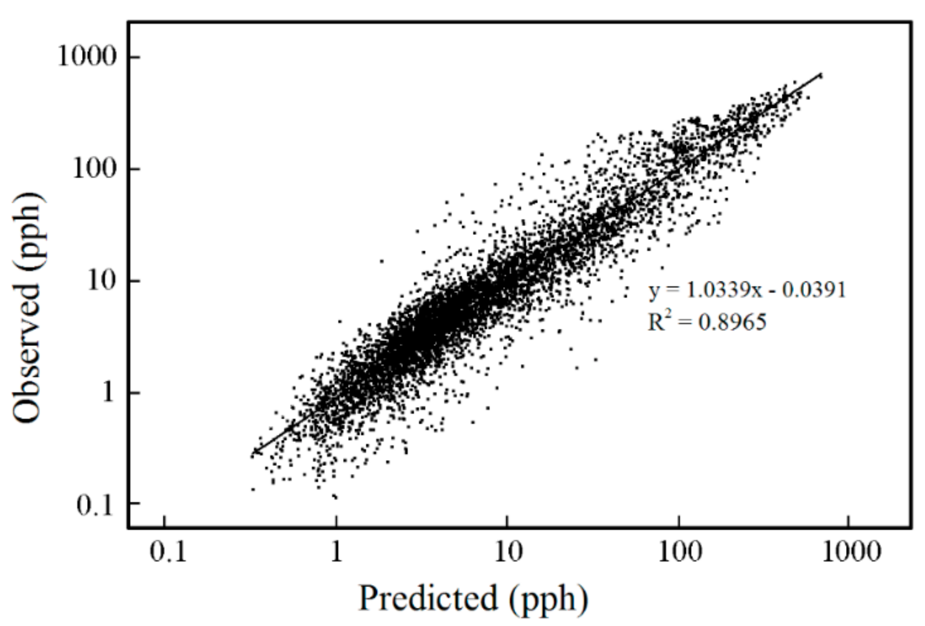
The accuracy assessment of estimated population products was constructed using summed gridded population count value and compared with census data, which were at the township level. In this study, we only analyzed the prediction of 2010 because the township level demographics in 2000 were unavailable. The result (Figure 3) shows that the resident population density (pph: population per hectare) is strongly correlated with the simulation result (R² = 0.8965, p < 0.01). Thus, the gridded population distribution is acceptable.

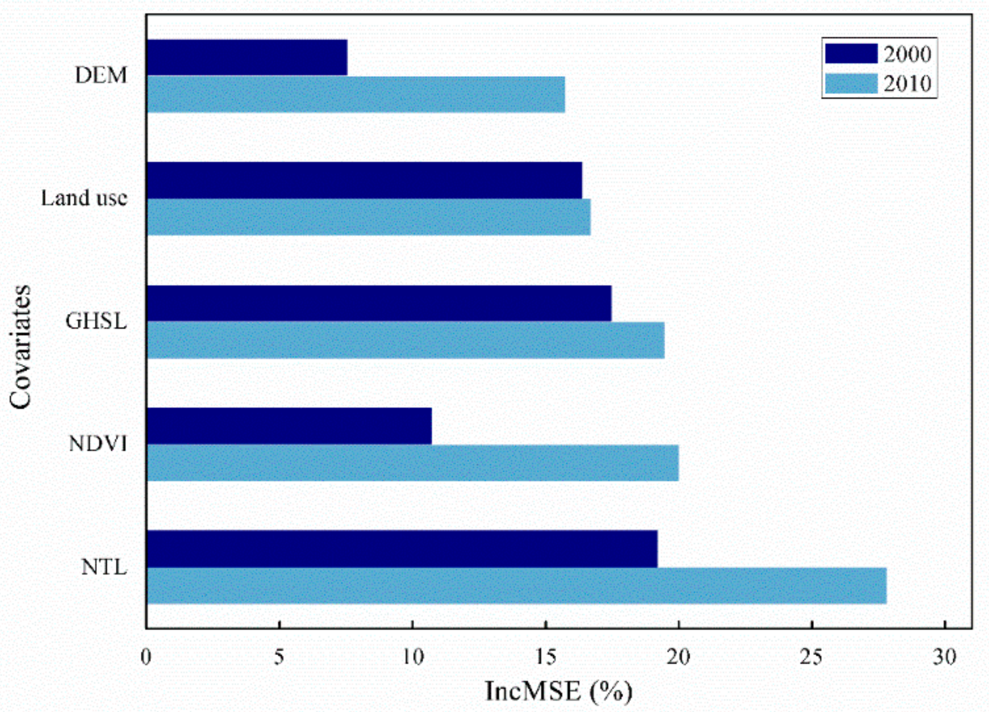
Figure 4 highlights the covariate importance for each modeled year. The high value of percent IncMSE indicates the variable that is important in the OOB cross-validation process [68] “NTL” is substantially important for 2 years and even becomes increasingly essential in 2010. The importance of the remaining four covariates is similar in 2010, but DEM and NDVI slightly contribute to the prediction of 2000.

4.2. Spatial Pattern of SRI

After PCA, 33 county-level variables were reduced to seven factors, explaining approximately 76.5% (2000) and 80.1% (2010) of the variance. The KMO values of the overall matrix are greater than 0.8. The results of Bartlett’s test of sphericity for SR are significant (p < 0.001). This finding indicates that the selected variables are appropriate for PCA. On the basis of Kaiser criterion (eigenvalues greater than 1) and significant factor loading (greater than 0.5 or less than −0.5), we identified seven principle components for 2000: occupational structure, economic structure, demography, elderly population, ethnicity, education, and unemployment rate (

Table 3. SR factors in China’s coastal zone in 2000.

FAC	Name (% Explained Variance)	No. of Drivers	Sign	Explanatory Variables (Loading)
1	Occupational structure (34.358)	11	+	HHSIP (0.898), PPHS (0.864), EIIP (0.856), PNAP (0.849), PPCD (0.829), TIIP (0.813), PUP (0.750), AYED (0.683), PTIG (0.657), PHRS (0.653), NBHRP (0.616)
2	Economic structure (16.871)	8	+	SIIP (0.887), PIIP (−0.787), PSIG (0.758), RPCG (0.696), PPIG (−0.673), PCHA (0.552), PHWPW (0.543), PHWB (−0.504)
3	Demography (7.446)	6	−	NPGR (0.830), HOUSI (0.802), PHWT (0.743), SERA (0.626), PPAY (0.728), PHWK (0.601)
4	Elderly population (5.554)	3	+	HPAO (−0.825), PPAO (−0.650), WEPIP (0.578)
5	Ethnicity (4.436)	2	−	PMP (0.773), PCLA (0.685)
6	Education (4.213)	2	−	PIP (0.753), ANH (0.510)
7	Unemployment rate (3.656)	1	−	UNERA (0.551)

). In 2010, seven factors were extracted: occupational structure, economic structure, household size, elderly population, education, land utilization, and housing condition (

Table 4. Factors of social resilience in the coastal zone of China in 2010.

FAC	Name (% Explained Variance)	No. of Drivers	Sign	Explanatory Variables (Loading)
1	Occupational structure (34.353)	12	+	EIIP (0.893), HSSIP (0.892), TIIP (0.811), PPHS (0.768), UNRA (0.757), PNAP (0.745), PPCD (0.718), WEPIP (0.694), AYED (0.639), PUP (0.596), PTIG (0.583), NBHRP (0.560)
2	Economic structure (14.654)	7	−	SIIP (−0.801), PIIP (0.756), PSIG (−0.749), PPIG (0.748), PHWPW (0.696), PHWT (0.694), PHWB (0.638)
3	Household size (9.454)	4	+	HOUSI (−0.824), PPAY (−0.757), NPGR (−0.630), RPCG (0.565)
4	Elderly population (7.223)	5	+	PPAO (−0.791), SERA (0.737), HPAO (−0.707), PHWK (0.642), PHRS (0.571)
5	Education (5.311)	2	−	PIP (0.800), PCHA (0.599)
6	Land utilization (3.679)	2	+	PCLA (0.731), PMP (0.628)
7	Housing condition (3.321)	1	+	ANH (0.820)

). Among the driving factors, occupational structure emerged as the dominant one in 2000 and 2010.

The distribution maps (Figure 5) and transition matrix (

Table 5. Transition matrix of SRI in China’s coastal zone from 2000 to 2010 (unit: km²).

	2010	Very Low	Low	Medium	High	Very High
2000
Very low		1571.95	0.00	0.00	0.00	0.00
Low		7106.40	138,546.52	27,798.20	3343.20	0.00
Medium		0.00	41,830.45	176,952.52	21,799.88	0.00
High		0.00	0.00	6175.22	22,440.03	9342.58
Very high		0.00	0.00	0.00	5739.86	24,709.41

) of SRI show that the majority of the counties exhibit a low or medium level of SR. Regionally, the highly resilient counties are centered in Yangtze River Delta, Pearl River Delta, and Haihe River Basin. Other counties with high or very high values are dotted along the coastal zone. On the contrary, the counties with a low level of SRI are located in four main regions: Bohai Rim Region, north of Jiangsu Province, border of Fujian and Guangzhou Provinces, and Guangxi Province. The result obtained by the transfer matrix (Table 5) indicates that 74.73% of the regions had no change in their SRI levels, and only 12.78% had an increased resilience. This change is evident at the junction of Zhejiang and Fujian Provinces, indicating another concentration of high SR in 2010.

4.3. Spatial Pattern of SoVI

The SoVI scores for China’s coastal zone at a 250-m resolution were calculated (Figure 6) and statistics of Global Moran’s I were positive. The relative z-scores were greater than 2.54 (p < 0.05), indicating significant spatial clustering in 2000 SoVI (Moran’s I = 0.457) and 2010 SoVI (Moran’s I = 0.477). The overall concentration of social vulnerability slightly increased over the decade. The LISA cluster maps for SRI were drawn based on the local Moran’s I statistics to identify local spatial autocorrelation (Figure 7).

As shown in Figure 6, most regions in China’s coastal zone tend to exhibit very low or low level of social vulnerability. Two cold clusters (L–L) can be identified (Figure 7): one is the Hainan province, and the other is located in southern Liaoning. However, the clustered counties at low vulnerability in 2000 (37 counties or 12.67%) are evidently more than 2010 (12 counties or 4.11%). This finding indicates that the social vulnerability of coastal China is increasing in that decade. Counties, except the several small spots, with a significantly high value (H–H) in 2000 are clustered in southern Jiangsu, eastern Guangzhou Province, and Pearl River Delta (Figure 7); however, the southern Jiangsu is less vulnerable than the other clusters (Figure 6). In 2010, the number of tracts in the H–H cluster is barely changed and mainly distributed in Yangtze and Pearl River Deltas. Apart from these high vulnerability clusters, a large number of high-value spots scatter along the coast zone, especially in Shandong and the southeast coast (Figure 6).

4.4. Trend Variations in SoVI

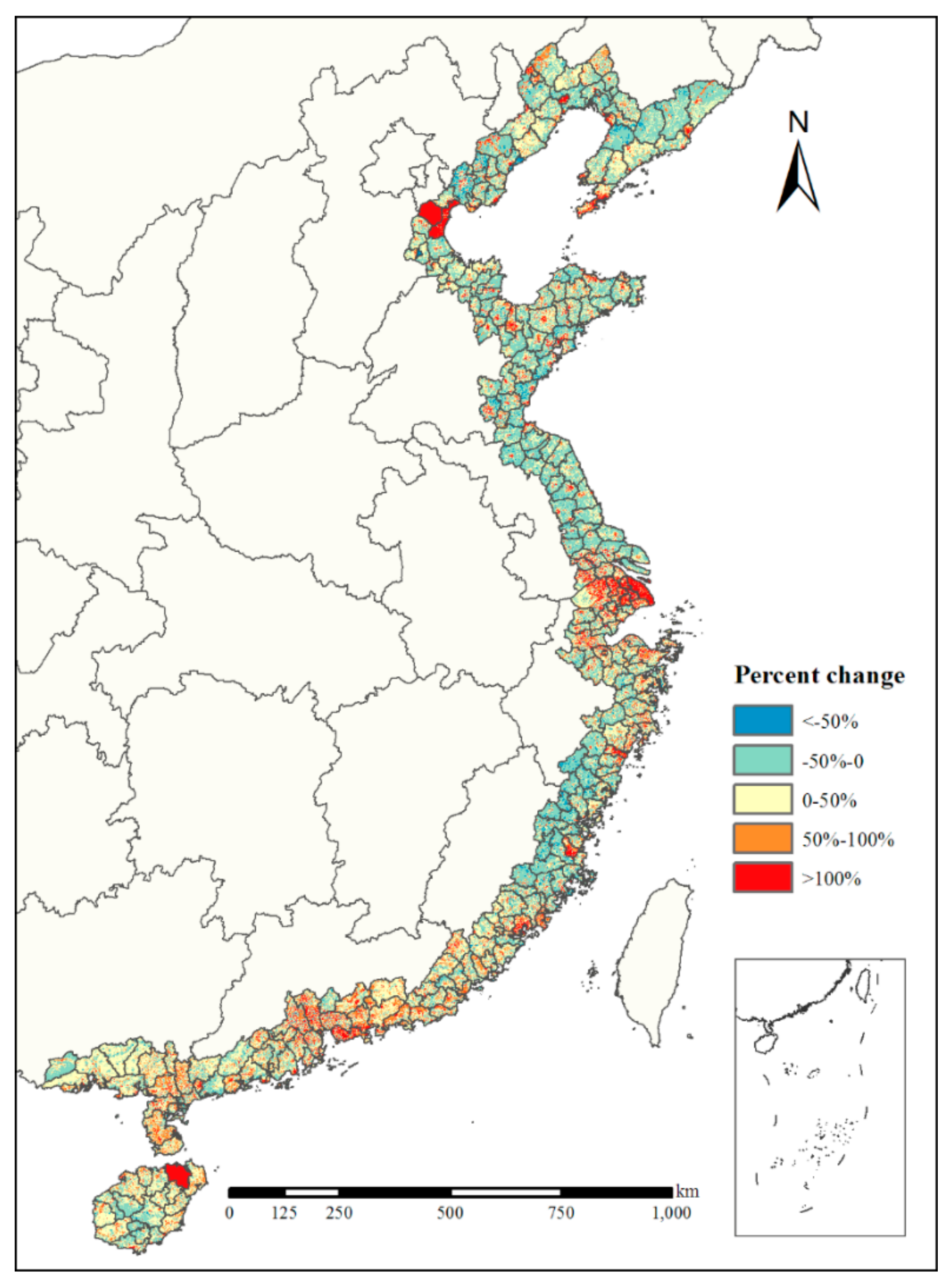
The transition matrix of SoVI (

Table 6. Transition matrix of SoVI in China’s coastal zone from 2000 to 2010 (unit: km²).

	2010	Very Low	Low	Medium	High	Very High
2000
Very low		240,697.50	39,306.75	1919.56	601.25	67.13
Low		27,740.56	108,871.38	15,724.13	3854.44	1183.25
Medium		221.19	10,172.56	12,602.13	5433.13	3462.44
High		1.69	415.13	2138.38	3001.13	5121.38
Very high		0.00	6.75	165.94	477.19	2545.94

) shows that the dissemination areas with level change are 118,012.81 km², accounting for only 24.30% of the coastal zone. Among the areas, the level rising area accounts for 64.97%. Therefore, the increasing trend of social vulnerability is evident in the decade.

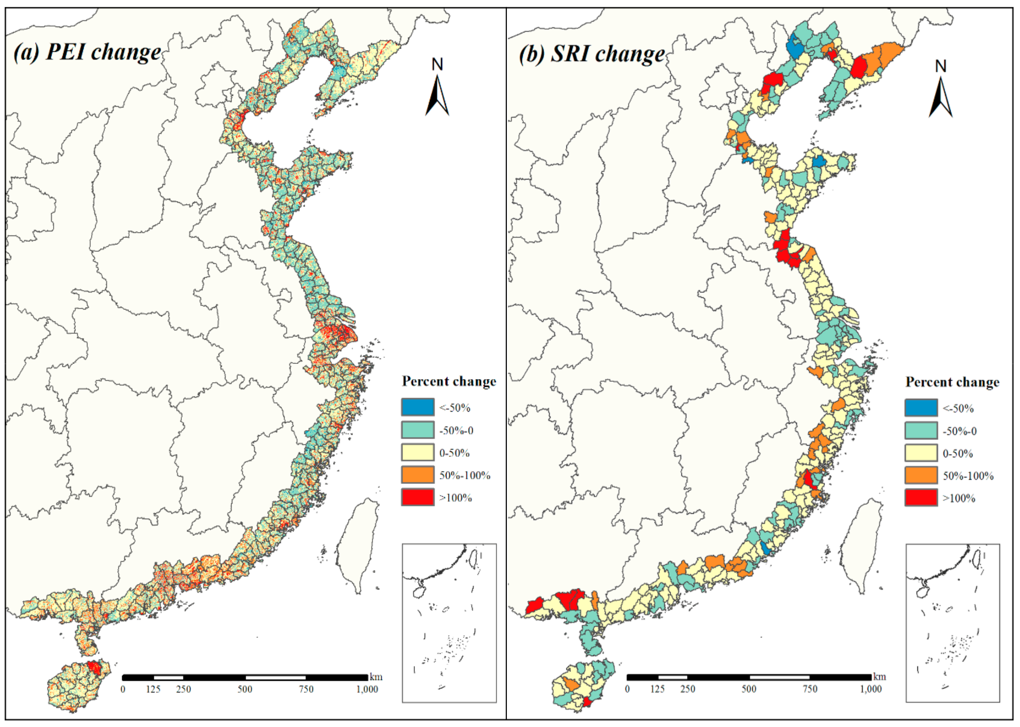
The percent changes were calculated for PEI (($PE{I}_{2010}-PE{I}_{2000})/PE{I}_{2000}$), SRI (($SR{I}_{2010}-SR{I}_{2000})/SR{I}_{2000}$), and SoVI (($SoV{I}_{2010}-SoV{I}_{2000})/SoV{I}_{2000}$), expressing the evolution of the social vulnerability driven by PE and SR in the study area (Figure 8 and Figure 9). This undertaking was initiated to obtain a detailed and relative understanding of oscillations that occurred between 2000 and 2010. A spatial autocorrelation of SoVI percent change also exists across China’s coastal zone (Moran’s I = 0.339). As shown in Figure 8, 56% dissemination areas of the coastal zone exhibit improved vulnerability. The noticeable changes are emphasized in Tianjin, Yangtze River Delta, and Pearl River Delta—the concentration of dissemination areas in which SoVI dramatically increased by over 100%. In these three hot spots, the PE has increased (Figure 9a), and their corresponding SR has a downward trend (Figure 9b) even at a high level (Figure 5). Therefore, the social vulnerability of these three economically developed regions increased in the decade. However, the LISA cluster map (Figure 10) shows that the high value clusters (H–H) are only located in the Yangtze River Delta. Tianjin is categorized as an H–L outlier, which means that the isolated municipal district with high vulnerability increase is surrounded by low or negative vulnerability increasing counties. The dissemination areas with significant increase in the Pearl River Delta are scattered. Such condition may be the reason why the Pearl River Delta is a statistically insignificant cluster. Counties with a decreasing social vulnerability cluster in the northern Jiangsu and border of Zhejiang and Jiangsu Provinces (Figure 10). The SR of these regions is increasing (Figure 9b), whereas the PE decreases as a whole (Figure 9a). In eastern Liaoning and Guangxi Province, the SR and PE have increased (Figure 9); however, the former has a negative change (less vulnerable), and the latter has a positive one (more vulnerable) (Figure 8). PE and SR have different effects in various regions. In this study, SR in the eastern part of Liaoning had a relative change, whereas PE in Guangxi Province was a dominant driving factor.

5. Discussion

The spatial distribution maps and transfer matrixes demonstrate that most counties are considered “very low” or “low” in terms of PEI and SoVI in 2000 and 2010. Without evident regional shift, the clusters with a maximum value of PE and social vulnerability are located in Tianjin, Yangtze River Delta, and Pearl River Delta where the SR is categorized as high level. Here, the driving factor was PE. Most counties belong to “low” and “medium” levels of SRI. Therefore, the SR of the study area still has a large room for improvement. In previous studies on China’s coastal zone, Ge et al. [48] proposed that counties with high adaptive capacity and low sensitivity were concentrated in Yangtze and Pearl River Deltas. Su et al. [47] identified Tianjin, Shanghai, Guangzhou, Shenzhen, and Dongguan as extreme groups of high adaptability. Guangzhou, Tianjin, and Shanghai were less sensitive to hazards. These results are consistent with the SRI spatial pattern proposed in the present paper.

The temporal analysis suggests the following: (1) The spatial correlation in 2010 was slightly stronger than that in 2000. Such variation may be the result of accelerated urbanization: the rapid development of urban regions leads to the concentration of population and resources. (2) The percent change of SoVI from 2000 to 2010 indicates an upward trend in social vulnerability and is emphasized in Yangtze River Delta. The identification regarding highly vulnerable and rapidly changing regions has practical significance for protection and risk mitigation.

The dominant factors contributing the most to SR can be discovered through PCA because of high explained variance [49]. Accordingly, stakeholders are provided with a benchmark reference to enhance SR and reduce social vulnerability. Occupational and economic structures are the top two drivers that represent approximately 50% of variance in 2000 and 2010. Occupation and economy are closely related: if a large number of people work in tertiary industries, then the economy will greatly advance [83]. The tertiary industry incudes transportation, warehousing, and postal services; information transmission, software, and information technology services, wholesale and retail, financial industry, leasing and business services, and scientific research and technical services [84]. Shanghai, Tianjin, Guangzhou, and Zhejiang chartered by high GDP are prosperous regions of the tertiary industry in China’s coastal zone [85], the SR of which is also at a high level (Figure 5). Therefore, a society’s capability to resist disruptive events can be strengthened by accelerating industrial transformation and developing production and service industry.

Social vulnerability is the product of the social inequality and historic patterns of social relations [29,62] that influence or shape the susceptibility and adaptive capacity of various groups to harm. Social inequality, which includes economic vitality, families and households, age, infrastructure, literacy, and disability, can be improved by socially based services such as housing, welfare, health, and education. However, historical factors, such as class, ethnicity, race, and gender, manifest as deeply embedded social structural barriers that are resistant to change. Although social disparities are inadvertently perpetuated, we can reduce it through transnational flows of capital/goods, information/ideas [86], and implementation of new social policies.

Significant differences can be explored between urban and rural areas. The economically developed regions, such as Yangtze and Pearl River Deltas, and the metropolises, including Tianjin, Qingdao, Suzhou, Fuzhou, Xiamen, and Shantou, have a high SoVI. The percent change of SoVI in these places is almost at the maximum level. Such trend can be explained by the “urban restructuring” thesis [63,87,88], which focused on the influences of capital and labor restructuring on urbanization. The rapidly growing economy and large demand for labor attract a sizeable migrant population pour into metropolises. Accordingly, the PE of those areas increases and the less developed regions may face hardship. The migrants become vulnerable because the presence of inequality makes it difficult for them to find good paying jobs or affordable housing [87,88] and participate in a political planning process for having their voice heard [62]. Migrants tend to cluster in highly developed but vulnerable areas. Consequently, the vulnerability of such migrants in the region increases. In this context, the government must promote inter-regional coordinated development and pay great attention to the floating population referring to equality [89]. The high-resolution distribution patterns exhibit that hot spots almost concentrate in the downtown of each administrative unit. Developing suburban and satellites can alleviate pressure in the city center and reduce vulnerability.

Our study still has certain limitations. Data availability is a crucial factor during variable selection, especially in the third level of Chinese administrative hierarchy. In this study, we mainly used the fifth (2000) and sixth (2010) national population census data, which are the latest and highly accurate data that we could obtain to simulate SR at a county level. Thirty-three variables were selected to calculate SR, but they were insufficient. Several indicators were excluded because of certain limitations, such as income and consumption level, infrastructure construction, individual health status, transportation and communication facilities, and disaster awareness. The limitations can also lead us to rely on readily available variables, which are inevitable to be overlapped; however, they are not the highly appropriate indicators for social vulnerability [14,49,56].

The SoVI has been broadly applied to reflect multidimensionality, reduce complexity, and visualize results. However, whether the pre-event descriptions correspond to post-disaster outcomes is an ongoing issue. Few attempts to validate the SoVI metric were found, and extreme event losses have been regarded as a frequently proposed approach [40,90,91,92]. Cutter et al. [40] suggested that SoVI in a post-event situation, such as Hurricane Katrina, can be validated by comparing the losses and recovery result of different affected regions with the previously calculated SoVI. Rufat et al. [90] compared the outcomes of Hurricane Sandy with the SoVI constructed by four types of models. However, the correlation coefficients were low. The proposed method assumed that when facing the same grade pressure, the economic loss is great if the social vulnerability of a region is high, which is seldom the case [40,48], because natural disasters are geographically heterogeneous. Moreover, the poor individuals are sensitive, but they do not have much to lose.

Consistency is a prerequisite for scientific assessments [54]; thus, the same indicators were selected in 2000 and 2010 in this study. However, the same parameters may not capture changes that happened in the decade [8]—new and important factors may be affecting social vulnerability in 2010. We tried to make indicators comprehensive to remedy this recognized defect. However, deficiencies still persist due to data limitations. Subjectivity and arbitrariness are inevitable when selecting variables. Thus, the established evaluation index system should be revised and further calibrated when it is applied to other cases [47].

6. Conclusions

This study developed a social vulnerability assessment metric for China’s coastal zone at the grid level. The quantitative indicator models of social vulnerability were based on two dimensions: PEI, which expresses the exposure degree of a system, and SRI, which refers to the system’s capability to absorb, adapt to, and recover from a disturbance. Multisensor remote sensing data, demographic and socioeconomic data, GIS techniques, RF model, and PCA were used to develop 2000 and 2010 SoVIs. The spatial distribution and LISA clustering maps of SoVI indicate that dissemination areas with high social vulnerability values are concentrated in Yangtze River Delta, Pearl River Delta, and eastern Guangzhou. Such areas are densely populated and economically prosperous. The maximum increase occurs in the Yangtze River Delta, which is categorized as the H–H cluster, denoting the region that deserves great attention.

The spatiotemporal comparison analysis of the SoVI value and the two dimensions that compose social vulnerability (PE and SR can be an effective tool for risk reduction planning. However, whether the indicator model of social vulnerability truly represents such abstract concept remains unaddressed. Thus, the validation method is worthy of in-depth research in the future.

References

- Balk, D.; Montgomery, M.R.; Mcgranahan, G.; Kim, D.; Mara, V.; Todd, M.; Buettner, T.; Dorélien, A. Mapping Urban Settlements and the Risks of Climate Change in Africa, Asia and South America; IIED: London UK; UNFPA: New York, NY, USA, 2009. [Google Scholar]
- Small, C.; Nicholls, R.J. A Global Analysis of Human Settlement in Coastal Zones. J. Coast. Res. 2003, 19, 584–599. [Google Scholar]
- Nguyen, T.T.X.; Bonetti, J.; Rogers, K.; Woodroffe, C.D. Indicator-based assessment of climate-change impacts on coasts: A review of concepts, methodological approaches and vulnerability indices. Ocean Coast. Manag. 2016, 123, 18–43. [Google Scholar] [CrossRef] [Green Version]
- Hugo, G. Future demographic change and its interactions with migration and climate change. Glob. Environ. Chang. 2011, 21, S21–S33. [Google Scholar] [CrossRef]
- Neumann, B.; Vafeidis, A.T.; Zimmermann, J.; Nicholls, R.J. Future Coastal Population Growth and Exposure to Sea-Level Rise and Coastal Flooding—A Global Assessment. PLoS ONE 2015, 10, e0118571. [Google Scholar] [CrossRef] [PubMed]
- Adger, W.N.; Hughes, T.P.; Folke, C.; Carpenter, S.R.; Rockström, J. Social-Ecological Resilience to Coastal Disasters. Science 2005, 309, 1036–1039. [Google Scholar] [CrossRef] [PubMed] [Green Version]
- Nicholls, R.J. Coastal flooding and wetland loss in the 21st century: Changes under the SRES climate and socio-economic scenarios. Glob. Environ. Chang. 2004, 14, 69–86. [Google Scholar] [CrossRef]
- King, D. Uses and Limitations of Socioeconomic Indicators of Community Vulnerability to Natural Hazards: Data and Disasters in Northern Australia. Nat. Hazards 2001, 24, 147–156. [Google Scholar] [CrossRef]
- Kijko, A.; Smit, A.; Papadopoulos, G.A.; Novikova, T. Tsunami Hazard Assessment of Coastal South Africa Based on Mega-Earthquakes of Remote Subduction Zones. Pure Appl. Geophys. 2018, 175, 1287–1304. [Google Scholar] [CrossRef]
- Galassi, G.; Spada, G. Sea-level rise in the Mediterranean Sea by 2050: Roles of terrestrial ice melt, steric effects and glacial isostatic adjustment. Glob. Planet. Chang. 2014, 123, 55–66. [Google Scholar] [CrossRef]
- Torresan, S.; Critto, A.; Rizzi, J.; Marcomini, A. Assessment of coastal vulnerability to climate change hazards at the regional scale: The case study of the North Adriatic Sea. Nat. Hazards Earth Syst. Sci. 2012, 12, 2347–2368. [Google Scholar] [CrossRef]
- Pickering, M. The Impact of Future Sea-Level Rise on the Tides. Ph.D. Thesis, University of Southampton, Southampton, UK, 2014. [Google Scholar]
- Zhong, Z. Feature and evaluation of natural disasters and environment in the coastal zones of China. Prog. Geogr. 1997, 16, 44–50. [Google Scholar] [CrossRef]
- Tapsell, S.; McCarthy, S.; Faulkner, H.; Alexander, M. Social vulnerability to natural hazards. Int. J. Disaster Risk Sci. 2010, 7, 111–122. [Google Scholar]
- Nguyen, L.D.; Raabe, K.; Grotte, U. Rural-Urban migration, household vulnerability, and welfare in Vietnam. World Dev. 2015, 71, 79–93. [Google Scholar] [CrossRef]
- Timmerman, P. Vulnerability resilience and collapse of society. A Review of Models and Possible Climatic Applications. Toronto, Canada; Institute for Environmental Studies, University of Toronto: Toronto, ON, CA, 1981. [Google Scholar]
- Füssel, H.-M. Vulnerability: A generally applicable conceptual framework for climate change research. Glob. Environ. Chang. 2007, 17, 155–167. [Google Scholar] [CrossRef]
- Toan, T.Q. Climate change and sea level rise in the mekong delta: Flood, tidal inundation, salinity intrusion, and irrigation adaptation methods. In Coastal Disasters and Climate Change in Vietnam; Elsevier: Amsterdam, The Netherlands, 2014; pp. 199–218. [Google Scholar] [CrossRef]
- Li, X.; Zhou, Y.; Tian, B.; Kuang, R.; Wang, L. GIS-based methodology for erosion risk assessment of the muddy coast in the Yangtze Delta. Ocean Coast. Manag. 2015, 108, 97–108. [Google Scholar] [CrossRef]
- Ford, J.D.; Smit, B. A framework for assessing the vulnerability of communities in the Canadian Arctic to risks associated with climate change. Arctic 2004, 389–400. [Google Scholar] [CrossRef]
- Pearce, T.; Smit, B.; Duerden, F.; Ford, J.D.; Goose, A.; Kataoyak, F. Inuit vulnerability and adaptive capacity to climate change in Ulukhaktok, Northwest Territories, Canada. Polar Rec. 2010, 46, 157–177. [Google Scholar] [CrossRef]
- Smit, B.; Wandel, J. Adaptation, adaptive capacity and vulnerability. Glob. Environ. Chang. 2006, 16, 282–292. [Google Scholar] [CrossRef]
- Turner, B.L.; Kasperson, R.E.; Matson, P.A.; McCarthy, J.J.; Corell, R.W.; Christensen, L.; Eckley, N.; Kasperson, J.X.; Luers, A.; Martello, M.L. A framework for vulnerability analysis in sustainability science. Proc. Natl. Acad. Sci. USA 2003, 100, 8074–8079. [Google Scholar] [CrossRef] [Green Version]
- Williamson, S.; Sharp, M.; Dowdeswell, J.; Benham, T. Iceberg calving rates from northern Ellesmere Island ice caps, Canadian Arctic, 1999–2003. J. Glaciol. 2008, 54, 391–400. [Google Scholar] [CrossRef]
- Cutter, S.L. Vulnerability to environmental hazards. Prog. Hum. Geogr. 1996. [Google Scholar] [CrossRef]
- Adger, W.N. Social Vulnerability to Climate Change and Extremes in Coastal Vietnam. World Dev. 1999, 27, 249–269. [Google Scholar] [CrossRef]
- Brooks, N. Vulnerability, Risk and Adaptation: A Conceptual Framework; Tyndall Centre for Climate Change Research Working Paper; Tyndall Centre for Climate Change Research: Cardiff, UK, 2003; Volume 38, pp. 1–16. [Google Scholar]
- Adger, W.; Brooks, N.; Bentham, G.; Agnew, M.; Eriksen, S. New Indicators of Vulnerability and Adaptive Capacity; Tyndall Centre for Climate Change Research: Norwich, UK, 2004. [Google Scholar]
- Cutter, S.L.; Boruff, B.J.; Shirley, W.L. Social Vulnerability to Environmental Hazards. Soc. Sci. Q. 2003, 84, 242–261. [Google Scholar] [CrossRef]
- Preston, B.L.; Stafford-Smith, M. Framing Vulnerability and Adaptive Capacity Assessment: Discussion Paper; CSIRO Climate Adaptation National Research Flagship: Aspendale, Australia, 2009. [Google Scholar]
- Preston, B.L.; Yuen, E.J.; Westaway, R.M. Putting vulnerability to climate change on the map: A review of approaches, benefits, and risks. Sustain. Sci. 2011, 6, 177–202. [Google Scholar] [CrossRef]
- Muler, M.; Bonetti, J. An Integrated Approach to Assess Wave Exposure in Coastal Areas for Vulnerability Analysis. Mar. Geod. 2014, 37, 220–237. [Google Scholar] [CrossRef]
- Rani, N.S.; Satyanarayana, A.N.V.; Bhaskaran, P.K. Coastal vulnerability assessment studies over India: A review. Nat. Hazards 2015, 77, 405–428. [Google Scholar] [CrossRef]
- McLaughlin, S.; Cooper, A. A Multi-scale coastal vulnerability index: A tool for coastal managers? Environ. Hazards 2010, 9, 233–248. [Google Scholar] [CrossRef]
- Eakin, H.; Luers, A. Assessing the Vulnerability of Social-Environmental Systems. Annu. Rev. Environ. Resour. 2006, 31, 365–394. [Google Scholar] [CrossRef] [Green Version]
- Ford, J.; Keskitalo, E.C.; Smith, T.; Pearce, T.; Berrang-Ford, L.; Duerden, F.; Smit, B. Case Study and Analogue Methodologies in Climate Change Vulnerability Research. Wiley Interdiscip. Rev. Clim. Chang. 2010, 1, 374–392. [Google Scholar] [CrossRef]
- Janssen, M.A.; Schoon, M.L.; Ke, W.; Bo, K. Scholarly networks on resilience, vulnerability and adaptation within the human dimensions of global environmental change. Glob. Environ. Chang. 2006, 16, 240–252. [Google Scholar] [CrossRef] [Green Version]
- Brooks, N.; Neil Adger, W.; Mick Kelly, P. The determinants of vulnerability and adaptive capacity at the national level and the implications for adaptation. Glob. Environ. Chang. 2005, 15, 151–163. [Google Scholar] [CrossRef]
- Adger, W.N. Vulnerability. Glob. Environ. Chang. 2006, 16, 268–281. [Google Scholar] [CrossRef]
- Cutter, S.L.; Finch, C. Temporal and spatial changes in social vulnerability to natural hazards. Proc. Natl. Acad. Sci. USA 2008, 105, 2301. [Google Scholar] [CrossRef] [PubMed]
- Adger, W.N.; Brown, K.; Nelson, D.R.; Berkes, F.; Eakin, H.; Folke, C.; Galvin, K.; Gunderson, L.; Goulden, M.; O’Brien, K. Resilience implications of policy responses to climate change. Wiley Interdiscip. Rev. Clim. Chang. 2011, 2, 757–766. [Google Scholar] [CrossRef]
- Lee, Y.-J. Social vulnerability indicators as a sustainable planning tool. Environ. Impact Assess. Rev. 2014, 44, 31–42. [Google Scholar] [CrossRef]
- Cutter, S.L.; Ash, K.D.; Emrich, C.T. The geographies of community disaster resilience. Glob. Environ. Chang. 2014, 29, 65–77. [Google Scholar] [CrossRef]
- Mahapatra, M.; Ramakrishnan, R.; Rajawat, A.S. Coastal vulnerability assessment using analytical hierarchical process for South Gujarat coast, India. Nat. Hazards 2015, 76, 139–159. [Google Scholar] [CrossRef]
- Leichenko, R.; O’Brien, K. The Dynamics of Rural Vulnerability to Global Change: The Case of Southern Africa. Mitig. Adapt. Strateg. Glob. Chang. 2002, 7, 1–18. [Google Scholar] [CrossRef]
- Chen, W.; Cutter, S.; Emrich, C.; Shi, P. Measuring social vulnerability to natural hazards in the Yangtze River Delta region, China. Int. J. Disaster Risk Sci. 2013, 4, 169–181. [Google Scholar] [CrossRef] [Green Version]
- Su, S.; Pi, J.; Wan, C.; Li, H.; Xiao, R.; Li, B. Categorizing social vulnerability patterns in Chinese coastal cities. Ocean Coast. Manag. 2015, 116, 1–8. [Google Scholar] [CrossRef]
- Ge, Y.; Dou, W.; Liu, N. Planning Resilient and Sustainable Cities: Identifying and Targeting Social Vulnerability to Climate Change. Sustainability 2017, 9, 1394. [Google Scholar] [CrossRef]
- Zhou, Y.; Li, N.; Wu, W.; Wu, J.; Shi, P. Local spatial and temporal factors influencing population and societal vulnerability to natural disasters. Risk Anal. 2014, 34, 614–639. [Google Scholar] [CrossRef] [PubMed]
- Nguyen, C.V.; Horne, R.; Fien, J.; Cheong, F. Assessment of social vulnerability to climate change at the local scale: Development and application of a Social Vulnerability Index. Clim. Chang. 2017, 143, 355–370. [Google Scholar] [CrossRef]
- De Oliveira Mendes, J.M. Social vulnerability indexes as planning tools: Beyond the preparedness paradigm. J. Risk Res. 2009, 12, 43–58. [Google Scholar] [CrossRef]
- Cutter, S.L. The landscape of disaster resilience indicators in the USA. Nat. Hazards 2015, 80, 741–758. [Google Scholar] [CrossRef]
- Yusuf, A.A.; Francisco, H. Climate Change Vulnerability Mapping for Southeast Asia; EEPSEA Special & Technical Paper; EEPSEA: Singapore, 2009. [Google Scholar]
- Fekete, A. Social vulnerability change assessment: Monitoring longitudinal demographic indicators of disaster risk in Germany from 2005 to 2015. Nat. Hazards 2018. [Google Scholar] [CrossRef]
- Merkens, J.-L.; Vafeidis, A. Using Information on Settlement Patterns to Improve the Spatial Distribution of Population in Coastal Impact Assessments. Sustainability 2018, 10, 3170. [Google Scholar] [CrossRef]
- Hu, K.; Yang, X.; Zhong, J.; Fei, F.; Qi, J. Spatially explicit mapping of heat health risk utilizing environmental and socioeconomic data. Environ. Sci. Technol. 2017, 51, 1498–1507. [Google Scholar] [CrossRef] [PubMed]
- Chen, Q.; Ding, M.; Yang, X.; Hu, K.; Qi, J. Spatially explicit assessment of heat health risk by using multi-sensor remote sensing images and socioeconomic data in Yangtze River Delta, China. Int. J. Health Geogr. 2018, 17, 15. [Google Scholar] [CrossRef] [PubMed]
- Li, K.; Chen, Y.; Li, Y. The Random Forest-Based Method of Fine-Resolution Population Spatialization by Using the International Space Station Nighttime Photography and Social Sensing Data. Remote Sens. 2018, 10, 1650. [Google Scholar] [CrossRef]
- Ye, T.; Zhao, N.; Yang, X.; Ouyang, Z.; Liu, X.; Chen, Q.; Hu, K.; Yue, W.; Qi, J.; Li, Z. Improved population mapping for China using remotely sensed and points-of-interest data within a random forests model. Sci. Total Environ. 2019, 658, 936–946. [Google Scholar] [CrossRef] [PubMed]
- Cutter, S.L.; Derakhshan, S. Temporal and spatial change in disaster resilience in US counties, 2010–2015. Environ. Hazards 2018, 1–20. [Google Scholar] [CrossRef]
- Sanchez, L.D. Social Vulnerability to Hurricane Disasters: Exploring the Effect of Place as a Mediating Factor. Ph.D. Thesis, The University of Texas at San Antonio, San Antonio, TX, USA, 2018. [Google Scholar]
- Thomas, D.S.K. Social Vulnerability to Disasters, 2nd ed.; CRC Press: Boca Raton, FL, USA, 2013. [Google Scholar]
- Kashem, S.B.; Wilson, B.; Van Zandt, S. Planning for Climate Adaptation. J. Plan. Educ. Res. 2016, 36, 304–318. [Google Scholar] [CrossRef]
- Ho, H.C.; Knudby, A.; Chi, G.; Aminipouri, M.; Lai, D.Y.-F. Spatiotemporal analysis of regional socio-economic vulnerability change associated with heat risks in Canada. Appl. Geogr. 2018, 95, 61–70. [Google Scholar] [CrossRef] [PubMed]
- Yin, J.; Yin, Z.; Wang, J.; Xu, S. National assessment of coastal vulnerability to sea-level rise for the Chinese coast. J. Coast. Conserv. 2012, 16, 123–133. [Google Scholar] [CrossRef]
- Liu, X.; Hu, G.; Chen, Y.; Xia, L.; Xu, X.; Li, S.; Pei, F.; Wang, S. High-resolution multitemporal mapping of global urban land using Landsat images based on the Google Earth Engine Platform. Remote Sens. Environ. 2018, 209, 227–239. [Google Scholar] [CrossRef]
- Tatem, A.J.; Adamo, S.; Bharti, N.; Burgert, C.R.; Castro, M.; Dorelien, A.; Fink, G.; Linard, C.; John, M.; Motana, L. Mapping populations at risk: Improving spatial demographic data for infectious disease modeling and metric derivation. Popul. Health Metr. 2012, 10, 8. [Google Scholar] [CrossRef]
- Gaughan, A.E.; Stevens, F.R.; Huang, Z.; Nieves, J.J.; Sorichetta, A.; Lai, S.; Ye, X.; Linard, C.; Hornby, G.M.; Hay, S.I.; et al. Spatiotemporal patterns of population in mainland China, 1990 to 2010. Sci. Data 2016, 3, 160005. [Google Scholar] [CrossRef]
- Sorichetta, A.; Hornby, G.; Stevens, F.; Gaughan, A.; Linard, C.; Tatem, A. High-resolution gridded population datasets for Latin America and the Caribbean in 2010, 2015, and 2020. Sci. Data 2015, 2, 150045. [Google Scholar] [CrossRef] [Green Version]
- Stevens, F.; Gaughan, A.; Linard, C.; Tatem, A. Disaggregating Census Data for Population Mapping Using Random Forests with Remotely-Sensed and Ancillary Data. PLoS ONE 2015, 10, e0107042. [Google Scholar] [CrossRef]
- Breiman, L. Random Forests. Mach. Learn. 2001, 45, 5–32. [Google Scholar] [CrossRef] [Green Version]
- Ma, T.; Zhou, C.; Pei, T.; Haynie, S.; Fan, J. Quantitative estimation of urbanization dynamics using time series of DMSP/OLS nighttime light data: A comparative case study from China’s cities. Remote Sens. Environ. 2012, 124, 99–107. [Google Scholar] [CrossRef]
- Lu, Z.Q.J. The Elements of Statistical Learning: Data Mining, Inference, and Prediction. J. R. Stat. Soc. Series A (Stat. Soc.) 2010, 173, 693–694. [Google Scholar] [CrossRef]
- Stafford, S.; Abramowitz, J. An analysis of methods for identifying social vulnerability to climate change and sea level rise: A case study of Hampton Roads, Virginia. Nat. Hazards 2017, 85, 1089–1117. [Google Scholar] [CrossRef]
- Tavares, A.O.; Barros, J.L.; Mendes, J.M.; Santos, P.P.; Pereira, S. Decennial comparison of changes in social vulnerability: A municipal analysis in support of risk management. Int. J. Disaster Risk Reduct. 2018, 31, 679–690. [Google Scholar] [CrossRef]
- Comrey, A.L.; Lee, H.B. A First Course in Factor Analysis; Psychology Press: Hove, UK, 2013. [Google Scholar]
- Renigier-Bilozor, M.; Wisniewski, R.; Bilozor, A. Rating attributes toolkit for the residential property market. Int. J. Strateg. Prop. Manag. Taylor Fr. J. 2017, 21, 307–317. [Google Scholar] [CrossRef]
- Renigier-Biłozor, M.; Wisniewski, R.; Kaklauskas, A.; Biłozor, A. Rating methodology for real estate markets-Poland case study. Int. J. Strateg. Prop. Manag. 2014, 18. [Google Scholar] [CrossRef]
- Sokal, R.R.; Oden, N.L. Spatial autocorrelation in biology: 1. Methodology. Biol. J. Linn. Soc. 1978, 10, 199–228. [Google Scholar] [CrossRef] [Green Version]
- Ord, J.K.; Getis, A. Testing for local spatial autocorrelation in the presence of global autocorrelation. J. Reg. Sci. 2001, 41, 411–432. [Google Scholar] [CrossRef]
- Rogerson, P. Statistical Methods for Geography: A Student’s Guide; Sage Publishing: Thousand Oaks, CA, USA, 2014. [Google Scholar]
- Anselin, L. Local indicators of spatial association—LISA. Geogr. Anal. 1995, 27, 93–115. [Google Scholar] [CrossRef]
- Liu, S.; Yu, H. Spatial Correlation Analysis Between Producer Services Agglomeration and Regional Economic Growth: An Empirical Study Based on 285 Cities in China. Mod. Financ. Econ. J. Tianjin Univ. Financ. Econ. 2018. [Google Scholar] [CrossRef]
- Coffey, W.J. The Geographies of Producer Services. Urban Geogr. 2000, 21, 170–183. [Google Scholar] [CrossRef]
- Zeng, G.; He, W. An Empirical Analysis of Regional Differences in the Development of China’s Tertiary Industry. Product. Res. 2007, 92–94. [Google Scholar] [CrossRef]
- Harrison, F.V. The Anthropology of Globalization: Cultural Anthropology Enters the 21st Century (Lwellen). Transform. Anthropol. 2010, 13, 57–58. [Google Scholar] [CrossRef]
- Castells, M.; Borja, J. Local and Global: The Management of Cities in the Information Age; Routledge: Abingdon, UK, 2013. [Google Scholar] [CrossRef]
- Sassen, S. Cities in a World Economy; Sage Publications: Thousand Oaks, CA, USA, 2018. [Google Scholar]
- Neil Adger, W.; Arnell, N.W.; Tompkins, E.L. Successful adaptation to climate change across scales. Glob. Environ. Chang. 2005, 15, 77–86. [Google Scholar] [CrossRef]
- Rufat, S.; Tate, E.; Emrich, C.T.; Antolini, F. How Valid Are Social Vulnerability Models? Ann. Am. Assoc. Geogr. 2019, 1–23. [Google Scholar] [CrossRef]
- Burton, C.G. A Validation of Metrics for Community Resilience to Natural Hazards and Disasters Using the Recovery from Hurricane Katrina as a Case Study. Ann. Assoc. Am. Geogr. 2015, 105, 67–86. [Google Scholar] [CrossRef]
- Sherrieb, K.; Norris, F.H.; Galea, S. Measuring Capacities for Community Resilience. Soc. Indic. Res. 2010, 99, 227–247. [Google Scholar] [CrossRef]
Figure 1.
Study area.
Figure 2.
Spatial distribution of the potential exposure index (PEI) in China’s coastal zone in 2000 (a) and 2010 (b).
Figure 3.
Scatterplots of the predicted and census population density at the township level in China’s coastal zone. A log10 transformation was conducted.
Figure 4.
Percent increase of mean squared error indicates the variable importance for RF regression.
Figure 5.
Spatial distribution of SRI in China’s coastal zone in 2000 (a) and 2010 (b).
Figure 6.
Spatial distribution of SoVI in China’s coastal zone in 2000 (a) and 2010 (b).
Figure 7.
LISA cluster map for SoVI in 2000 (a) and 2010 (b).
Figure 8.
Percent change of SoVI in China’s coastal zone from 2000 to 2010.
Figure 9.
Percent change of PEI (a) and SRI (b) in China’s coastal zone from 2000 to 2010.
Figure 10.
LISA cluster map for SoVI percentage change from 2000 to 2010.