Abstract
Continuous urban expansion worldwide has resulted in significant wetland degradation and loss. A limited number of studies have addressed the coupling of wetland and urban dynamics, but this relationship remains unclear. In this study, a time-varying methodology of predicting wetland distribution was developed to support decision-making. The novelty of the methodology is its ability to dynamically simulate wetland shrinkage together with urban expansion and reveal conflicts and potential tradeoffs under different scenarios. The developed methodology consists of three modules: a historical change detection of wetland and urban areas module, a spatial urban sprawl simulation and forecasting module that can accommodate different development priorities, and a wetland distribution module with time-varying logistic regression. The methodology was applied and tested in the Tonghu Wetland as a case study. The wetland and urban extents presented a spatially intersecting shift, where wetlands lost more than 40% of their area from 1977 to 2017, while urban areas expanded by 10-fold, threatening wetlands. The increase in the relative importance metric of the time-varying regression model indicated an enhanced influence of urban expansion on the wetland. An accuracy assessment validated a robust statistical result and a good visual fit between spatially distributed wetland occurrence probabilities and the actual distribution of wetland. Incorporating the new variable of urban expansion improved modeling performance and, particularly, realized a greater ability to predict potential wetland loss than provided by the traditional method. Future wetland loss probabilities were visualized under different scenarios. The historical trend scenario predicted continuously expanding urban growth and wetland shrinkage to 2030. However, a specific urban development strategy scenario was designed interactively to control the potential wetland loss. Consideration of such scenarios can facilitate identifying tradeoffs to support wetland conservation.
1. Introduction
Wetlands are considered unique and important ecosystems, supplying useful products, such as peat and food, and performing valuable ecosystem services, such as biodiversity support, water purification, runoff regulation, flood abatement, and carbon storage [1]. However, wetland ecosystems are among the most threatened ecosystems, in which agricultural reclamation, afforestation, and residential and commercial development have caused huge losses of wetland area [2,3]. It has been reported that the global extent of wetlands has declined by more than 50% in the 20th century [4]. The key services provided by wetlands are impaired when wetlands are degraded or lost [5]. This causes loss of hydrological function [6], aggravates water shortage [7], exacerbates flood risks under climate change [8], weakens the carbon sink and climate stabilizer function [9], leads to habitat fragmentation and loss of fish and wildlife protection, and further results in a decline in species [10]. Moreover, demands for land and water resources intensify wetland degradation and loss continues worldwide [2,11]. In policy- and decision-making, there is a great need to understand the process of wetland loss, including the causes of loss [12]. Wetland and other land-use types compete with one another, and modeling their dynamics is necessary to support wetland conservation and restoration.
Multiple models for simulating land-use dynamics have been developed and applied to provide a platform for approximating land-use trajectories and projecting future change [13,14,15,16]. These models have ranged from those using pattern-based methods to those using structural or process-based methods [17,18], and five key types of modeling approaches have been identified [17]. The first type is machine learning models, which use statistical methods to simulate the relationships between land uses and variables and project the land-use changes using a spatially explicit allocation procedure. An example is the conversion of land use and its effects at small regional extents model (CLUE-S) [19] and its adapted versions [20,21]. The second approach is the cellular automata model, which is a cell-based land-use simulation system governed by combining maps of likelihood with spatial interaction effects [15]. The third and fourth types are economic models, sector-based economic models and spatially disaggregated economic models, and describe the land change as a market process [17]. The fifth type, agent-based modeling, consists of a number of ‘agents’ and flexibly incorporates the influence of human decision-making on land use [18,22]. These models simulate the land system process under different strategies.
Using land-use change modeling approaches, mainly including machine learning models with statistical methods and the cellular automata model, previous studies have performed wetland distribution and change simulation. Especially, numerous statistical methods, including the logistic regression model, maximum entropy approach, SimWeight machine learning procedure, and random forests model, have been utilized in previous studies. The logistic regression model is a non-linear regression analysis of the relationship between explanatory variables and binary response variables for calculating wetland occurrence probability [23,24,25,26]. The maximum entropy approach simulates and predicts how the distribution of wetlands would be modified in response to given environmental changes [27]. The SimWeight machine learning procedure uses the logic of the modified K-nearest neighbor to generate the wetland transition potential surface with the two classes of change and persistence [3]. The random forests model builds multiple decision trees, with each tree containing a random subset of variables to predict wetland distribution by a machine learning algorithm [28,29]. The cellular automata model generalizes the transition rules of cells by a self-adaptive method and neighbor conditions to model wetland change [30,31]. These models, consisting of different mathematical principles and model settings, have been used with different levels of model fitness in previous studies. Improving model performance calls for better quantification of the relationship between the driving forces and wetland change, particularly, precisely depicting the temporal and spatial details of the main driving factors.
Among the numerous driving factors, human disturbance, one key cause of wetland loss, changes dynamically within a range of intensities, and its influence on wetlands is also altered. However, among the aforementioned model applications, few studies simulating the wetland change process have simultaneously taken dynamic human activities into consideration [23,25]. To project wetland distribution, previous models have used data of driving factors at several periods to quantify changes in human activity [23,25], but have lacked the ability to forecast future change in human activity and its impact on wetlands. Most studies have built static models, assuming the influence of human activity to be a constant [26,27,28,29,30,31]. Limitations in the quantification and detection of dynamic human activity can easily lead to bias and uncertainties in model performance, especially when forecasting the future trend of wetlands under increasing pressure of anthropogenic disturbance [26,28]. In particular, urbanized areas, characterized by rapid population growth and spatial expansion in the past century, and likely continuing into the future [32], have had a dramatic and intense impact on wetland shrinkage [33,34,35]. Human disturbance within and near urbanized areas, such as the building of roads, utility corridors, and houses; dumping, filling, channelizing, and dredging; and the construction of drainage ditches and control dams, causes wetland degradation or loss [12]. Thus, the construction of a time-varying method of the intersecting dynamics of wetlands and human activity can better reveal the underlying drivers of wetland dynamics, and thus improve simulation accuracy.
However, the models that have been developed and applied recently project changes in wetlands [24,28,29,30,31] and urban extents [36,37] separately. Urban expansion has been simulated by extensive models, such as cellular automata, artificial neural networks, fractal geometry, linear/logistic regression, and agent-based models [38]. The slope, land use, exclusion, urban extent, transportation, and hillshade (SLEUTH) model is a modified cellular automata model that relaxes the many classic cellular automata limitations [15,37]. As one of the popular urban growth models, the SLEUTH model has been applied broadly to many study areas to simulate historic urban growth [39]. With its flexibility of output, the SLEUTH model has provided an opportunity for its integration with wetland dynamics models for a new methodology.
Thus, the objective of this study was to develop a novel methodology, named the time-varying wetland shrinkage and urban expansion (TVWSUE) methodology, to quantify and explore how urban growth has influenced wetland change. The TVWSUE methodology can detect the historical changes of wetland and urban extent, explore the time-varying impacts of driving factors on wetland shrinkage, and forecast future changes in wetlands. The Tonghu Wetland, which has experienced significant wetland loss under rapid urbanization in the past four decades, was selected as the study area. The methodology was applied and tested to simulate the wetland change from 1977 to 2030. The structure of this manuscript is organized into several sections. The next section begins with information about the study area and data, followed by a description of TVWSUE methodology and its application and validation. The third section of this paper presents the results of the TVWSUE execution and performance for the historical wetland shrinkage and urban expansion, as well as future forecasts of shrinkage and expansion under scenario settings. The advantages, deficiencies, and potential future applications of our TVWSUE methodology are discussed in the fourth section, which is followed by a conclusion as the fifth section.
2. Materials and Methods
2.1. Study Area
The Tonghu Wetland is the largest inland wetland in the Pearl River Delta, the frontier of reform and development, and one of the three most developed regions in China [40]. The study area lies approximately within the latitude and longitude ranges of 22°58′20″ to 23°4′43″ N and 114°7′10″ to 114°18′30″ E and has an area of 150.5 km2 (Figure 1). It belongs to the Pearl River Basin and includes Tonghu Lake, with an area 6.9 km2, in the center. The Tonghu Wetland consists of plains and depressions, with low elevations ranging from 2–198 m. The area is located within the south subtropical monsoon climate zone, which has both abundant sunshine and rainfall. Calculated from the rasterized precipitation and temperature data from 1990 to 2015 from the Resource and Environment Data Cloud Platform (http://www.resdc.cn/), the mean annual precipitation is ca. 2000 mm and the mean annual temperature is ca. 23 °C. According to the Genetic Soil Classification of China, three principal soil types occur here: latosolic red soil, tidal sand soil, and paddy soil.
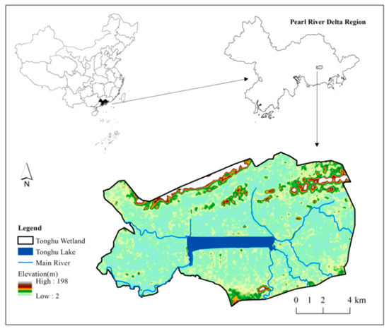
Figure 1.
Location and scope of the Tonghu Wetland.
The administrative district of the Tonghu Wetland is located in Huizhou City, and the wetland is near Shenzhen and Dongguang. A land reclamation project of converting natural wetlands into artificial wetlands was implemented in 1966 [41]. Subsequently, since the Economic Reform and Liberalization Policy began in 1978, the natural and artificial wetlands have gradually eroded [42]. With this policy, China has become the world’s fastest-growing economy and has experienced unprecedented urbanization [43]. Additionally, these three cities have experienced significant urbanization, which has encroached upon the huge wetlands for the purposes of urban use. Thus, it is advantageous to apply the TVWSUE to the Tonghu Wetland.
2.2. Data Description and Processing
2.2.1. Classification System
Land uses, including the wetland and urban areas, were mapped by a classification system constructed to execute the TVWSUE. The wetlands classification system used in this study was based on the international system of the Ramsar Convention [44] and the wetlands classification criteria in China [45,46], as well as regional wetland characteristics and the resolution of the available remote sensing images. The wetlands were basically categorized as natural wetland and artificial wetland. Natural wetland types included river, lake, and marsh, and artificial wetland types included paddy field, pond, and channel. All types were considered together as the wetlands for model simulation.
Land-use maps were necessary for the urban growth simulation. To be consistent with the constructed wetland classification system, the land-use classification system was altered based on the widely used land-use classification system in China [47]. Seven land-use types were interpreted for the land-use map, namely, paddy field, dryland, forest, grassland, water area, urban extent, and unused land. A difference between the classifications was that farmland was divided into paddy field and dryland in our classification, where paddy field was one kind of artificial wetland. Finally, water area and urban extent were specially identified and subdivided. The wetlands included paddy field and water area, which were also further subdivided according to the wetland classification system. The urban extent included residential land, industrial and mining land, and road.
2.2.2. Data Sources and Processing
Extensive satellite sources and remote sensing images, such as System Pour l’Observation de la Terre 5 (SPOT 5), Landsat Multispectral Scanner (MSS), Thematic Mapper (TM), Operational Land Imager (OLI)/Thermal Infrared Sensor (TIRS), Moderate Resolution Imaging Spectroradiometer (MODIS) [2,3,45,48,49], have provided the ability to detect wetland shrinkage and urban expansion. The minimum detectable unit and spatial scale of wetland and urban extent and change were determined mainly by the spatial resolution of the satellite images, for example, the spatial resolution of SPOT 5 images is 10 m, that of Landsat TM is 30 m, and that of MODIS is 250 m. The temporal detection scale is determined mainly by image availability, for example, MODIS is available after 2000. Meanwhile, the series of Landsat MSS, TM, and ETM+ images have been used jointly to perform long-term change detection for decades, starting from 1970s [3,25]. With the long-term data continuity and compatibility of the Landsat program with its series of sensors (MSS, TM, ETM+, and OLI/TIRS) [50], Landsat MSS, TM, and OLI images were selected for interpreting the land uses of this study. Considering the remote sensing image availability, the five time nodes of 1977, 1986, 1993, 2006, and 2017 were selected for visual interpretation of the land-use maps.
The TM, ETM+, and OLI/TIRS datasets have been shown to be compatible in combination [51]. Thus, the selected images for 1986, 1993, and 2006 were Landsat TM images, and the image for 2017 was a Landsat OLI image. The image for 1977 was from Landsat MSS, because there were only Landsat MSS images in the 1970s. Although the lower spatial resolution and fewer spectral bands available in Landsat MSS than in the other Landsat sensors cause biases, the interpretation accuracy of MSS and the comparability between different sensors of the same Landsat program have been shown to be valid in previous case studies [52,53,54]. The visible and near-infrared bands of MSS were compounded to false-color images to interpret the land use visually [50]. All of the Landsat images were provided by and downloaded from the Global Visualization Viewer (GloVis, http://glovis.usgs.gov/). Detailed information of the Landsat images is shown in Table 1. Topographic maps were obtained from the Institute of Geographic Sciences and Natural Resources Research, Chinese Academy of Sciences, and were digitized and geometrically matched by us. The natural wetlands for 1977 from the remote sensing interpretation were compared with those from the topographic maps, which had the same scale as that for the year 1965. The spatial locations of natural wetlands from the topographic maps and the remote sensing images were similar, but the boundaries of the two sources were not identical. When comparing the area of natural wetlands in 1965 to that in other time nodes, it was noted that the different data sources were skewed.

Table 1.
Landsat image description.
Preprocessing of the Landsat images included the application of geometric and atmospheric corrections from the Environment for Visualizing Images (ENVI) software (2015 Exelis ITT Visual Information Solutions). Thirty ground-control points taken from 1:50,000 topographic maps were selected. According to the ENVI Programmer’s Guide, the quadratic polynomial model was used for the geometric correction, which established the relationship between the position of the image pixel and the geographic coordinates of ground control points. The cubic convolution resampling technique was used to project the images according to the Universal Transverse Mercator (UTM) system, WGS84. It produced a root-mean-square spatial positioning error of less than 0.5 pixels for each image. Atmospheric corrections were performed using the FLAASH module.
To simulate the urban expansion, transportation network, slope, and hillshade datasets were also collected. The transportation networks for 1986, 1993, 2006, and 2017 were provided by the Transportation Department of Huizhou. The slope and hillshade data were calculated from the elevation determination, with a spatial resolution of 30 m, provided from the Global Topography Database of the Geospatial Data Cloud site (http://www.gscloud.cn/).
2.3. TVWSUE Methodology
Demands for economic development, population growth, and ecological protection prompt the completion of different land uses, which significantly influence the planet’s land surface [55]. To model the two intersecting land-use dynamic processes of wetland and urban area, the TVWSUE was developed with sequential operations by combining Geographic Information System (GIS) techniques, an urban expansion simulation model, and statistical methods. The novelty of our methodology is its time-varying and intersecting simulation ability, which allows it to couple wetland shrinkage with urban expansion simultaneously. The methodology consisted of three modules (Figure 2). The first module was the historical change detection module for mapping the temporal and spatial extents of wetlands and urbanization. With the constructed wetland classification system and the multiple sources of remote sensing images, the two datasets of historical wetland shrinkage and urban expansion trajectories were detected by the spatial analysis techniques. The second module simulated the temporal and spatial extent of urbanization. The SLEUTH model, a common model for simulating urban growth [15,37], was applied in this module. The acronym SLEUTH is derived from the initials of the six required input data, slope, land use, exclusion, urban extent, transportation, and hillshade. The exclusion data indicate specified areas limited to urban development and excluded in the model simulation. The derived historical data were used to calibrate the module and forecast urban sprawl. The third module, the wetland shrinkage projection module, incorporated the urban expansion result to forecast the distribution of wetlands dynamically. The time-varying explanatory variables, including the temporal surface hydrology and urban expansion, were collected and calculated. On the basis of multiple explanatory variables, the dynamic logistic regression model was constructed to simulate wetland distribution probabilities. Under future scenario design, the intersection of urban expansion and wetland shrinkage was investigated with different management strategies and priorities. Our model is hypothesized to obtain a better approximation of the wetland shrinkage process and an improved model fit.
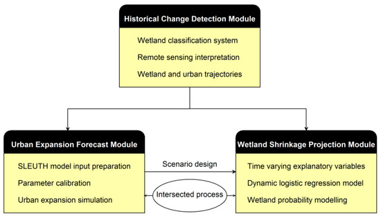
Figure 2.
Conceptual framework of the time-varying wetland shrinkage and urban expansion (TVWSUE) methodology for intersected processes of wetland shrinkage and urban expansion. SLEUTH, slope, land use, exclusion, urban extent, transportation, and hillshade.
2.3.1. Historical Change Detection Module
The historical change detection module is the basic procedure of the TVWSUE. Two key historical datasets—spatial distributions of wetland and urban extent—were extracted from a series of Landsat images and topographic maps at five time nodes within the period of 1977–2017. On the basis of the spatial overlying technique in ESRI ArcGIS 10.0, the historical change trajectories of natural wetland and new urban extent were detected and mapped for construction of the wetland change simulation model. Also, the cross-tabulation analysis of wetlands changing to other land uses between two adjacent time nodes was identified by the spatial overlaying technique. In particular, the transition from wetlands to urban uses was examined to explore their intersecting relationship. The new extent of urban expansion and its impact on wetland loss were quantified in our methodology. The spatial distribution of natural wetlands reflected the physical geomorphology, influenced the surface hydrological link and confluence area, and was further related to the distribution of wetlands [23]. Thus, the historical change trajectories of natural wetland and urbanization were identified by the following expressions:
where the NWs and NUs denote the historical trajectories of natural wetland and new urban extent, respectively; NWt1, NWt2, and NWn denote the natural wetland at the time nodes of t1, t2, and tn, respectively; and NUt1, NUt2, and NUn denote the new urban extent at the different time modes. Five time nodes were identified in this study, that is, t1 = 1977, t2 = 1986, t3 = 1993, t4 = 2006, and t5 = 2017.
On the basis of the interpretation marks from the field survey and their characteristics in the false-color composite images, the polygons of seven land-use types in the five time nodes were drawn manually by us in ESRI ArcGIS 10.0. In addition, the spatial distribution of natural wetlands in 1965 was mapped from topographic maps. The spatial distributions of natural wetland and urban extent at the five time nodes were extracted from the topographic maps and remote sensing images. Then, NWs and NUs were produced by the spatial overlaying technique, in which the spatial distributions of urban extent at two adjacent time nodes were overlain and the new urban extent was highlighted and identified. Particularly, Tonghu Lake was historically the largest natural wetland in the study area, but its shape has been modified artificially since 1965. The Tonghu links the main rivers and plays a key role in the regional surface hydrology. In the following analysis, the natural wetlands and Tonghu are referred to as “NWT”. The first module of the TVWUSE mapped the land uses from the remote sensing images, including the specified wetland and urban extents, for execution of the next two modules according to the classification system.
2.3.2. Urban Expansion Forecast Module
The second module incorporated the SLEUTH model to simulate the urban expansion through the sequence of data preparation, parameter calibration, and model prediction. The SLEUTH model has been implemented successfully in previous studies [15,39,56,57] and was selected to model urban expansion in our TVWSUE methodology. The SLEUTH model measures and simulates four modes of growth behavior, spontaneous growth, new spreading-center growth, edge (organic) growth, and road-influenced growth [37]. For calibration, the urban extents, land uses, and transport networks of 1986, 1993, 2006, and 2017, as well as the datasets of slope, exclusion, and hillshade, were used (Table 2). Unlike previous studies, in which all lakes and rivers were assigned as exclusion areas [15,39,56,57], only Tonghu Lake and the tributaries flowing into and out of the lake in 2017 were assigned as an exclusion in this case. This was done because Tonghu Lake is the largest lake in Guangdong Province and conversion of the lake or its tributaries to other uses is prohibited by the regional government [43]. The setting of this exclusion area was confirmed by the historical changes of these features, that is, the area where Tonghu Lake and its tributaries were not occupied by other land uses. All of the input data were resampled to the original spatial resolution of 30 m. Then, the urban extent for 2030 was forecast by the calibrated model. Although the planned road network is important for successful simulation using SLEUTH [58], the transportation network in the future scenario was not performed in this study because the newest road near Tonghu Lake was built in 2015–2017 and no additional new roads across the study area have been planned.
Table 2.
Input data for slope, land use, exclusion, urban extent, transportation, and hillshade (SLEUTH).
To improve the simulation performance of urban growth, the calibration is the most important stage for the SLEUTH model in the second module (Figure 2) This calibration procedure is done to choose the best values for the five control parameters approximating urban growth, that is, dispersion, breed, spread, slope resistance, and road gravity. On the basis of the input dataset, the control parameters were calibrated by an iterative method, which has been done commonly for application of the SLEUTH model in previous studies [56,57,59]. The detailed calibration information is briefly introduced below. The three phases of coarse, fine, and final resolution (120 m, 60 m, and 30 m, respectively) were carried out in the calibration. During the calibration process, urban growth was regenerated via different combinations of control parameters using Monte Carlo iterations. The step sizes of the control parameters at the coarse, fine, and final phases were 25, 5, and 1, respectively. A series of performance indices was calculated to assess the fit of simulated urban extents and referenced historic extents. Then, the Optimum SLEUTH Metric [60], a product of these performance indices, was used to narrow the range of parameters through the sequential calibration phase (coarse, fine, and final). Finally, the calibration parameters for simulating the urban growth of the study area were determined.
2.3.3. Wetland Shrinkage Projection Module
On the basis of the output of the first and second modules, the third module built a time-varying logistic regression model to simulate the wetland distribution. Given the uncertainty and complexity of the wetland dynamics process, the potential wetland change of a location was quantified by probability rules rather than a mechanism model, as used in previous studies. With its ability to incorporate explanatory variables and provide robust performance [23,24,25], the logistic regression model was selected as the core of the third module to model the wetland distribution.
The logistic regression model explores the relationship between explanatory variables and binary variables, in which the values of the input variable are 1 or 0, for example, the wetland exists or does not exist, respectively. In our study, the selected explanatory variables of wetland change included four categories (Table 3), that is, climate variable, topography factor, urban expansion influence, and surface hydrology factor. Distances to the initial urban extent, new urban extent, and natural wetland and Tonghu (NWT) indicated their influence, where a larger distance indicated a lower influence. The topography factors were considered fixed variables, which were related to intrinsic and historical hydrological characteristics of the study area. The factors of the climate variable, surface hydrology, and urban expansion were time-varying variables, which were believed to improve the model performance. With the small area of Tonghu Wetland and the abundant rainfall that occurs there, the climate variables presented low spatial variabilities and did not influence the wetland change (see the Results section). Future climate change scenarios were not used to simulate the wetland change in our model.
Table 3.
Descriptions of the explanatory variables for predicting wetland change.
With the specific setting of our TVWSUE methodology, the time-varying variables were distinguished in the dynamic logistic regression model as follows:
where Pt is the probability of wetland at the particular time node t; xf and xv are the fixed (topography factor) and varying variables (climate variable, surface hydrology factor, and urban expansion influence), respectively; nf and nv denote the number of fixed and time-varying variables, respectively; and βf and βv refer to the regression coefficients of the fth and vth fixed and varying variables, respectively. Using the historical change detection module and the urban expansion forecast module, the time-varying variables were calculated and used to build the time-varying logistic equation to execute the wetland shrinkage simulation module. The regression equations with time-varying variables to model the wetland distributions at 1986, 1993, 2006, and 2017 were fit in the SPSS18.0 statistical package.
To model the intersecting processes of urban expansion and wetland shrinkage in the future, the historical trend scenario of our TVWSUE methodology was forecast as the baseline, and a specific wetland conservation strategy was interactively designed to predict the future wetlands according to the result of the historical trend scenario. The tradeoff analysis between these processes can help resolve the conflict between urban development and wetland conservation.
2.4. Methodology Application and Validation
For the historical change detection module, 753 ground-reference data points in 2017, including 253 points from the field validation investigations with Global Positioning System (GPS) in 2017 and 500 points from high-resolution images from Google Earth in 2017, were used to assess the classification accuracy of the visually interpreted land-use map. Similarly, 500 points from high-resolution images from Google Earth in 2006 were used to assess the classification accuracy of the visually interpreted land-use map for 2006. Black-and-white aerial images were utilized to collect 500 reference points for validating the land-use classification result at 1986. The confusion matrix between the reference and interpreted results was used to calculate the overall accuracy and kappa coefficient (Table 4). The overall accuracies and kappa coefficients for 1986, 2006, and 2017 were 92.56%, 92.76%, and 92.10% and 0.918, 0.919, and 0.914, respectively, which validated the high accuracies of the land-use maps for 2006 and 2017. Without ground-reference data and high-resolution remote sensing images for the 1970s, 100 reference points were collected from the 1:50,000 topographic maps to validate the accuracy of the result for 1977 from the Landsat MSS image. The topographic maps were produced by aerial surveying and mapping in 1975, but only the boundary of natural wetlands was delineated. Thus, only the accuracy of the interpreted natural wetland in the land-use map for 1977 was tested, and the test resulted in an accuracy of 93.00%. Owing to the data availability, the accuracy of other land-use types was not tested in this study. In addition, the accuracy of the land-use map at 1993 was not assessed in this study because of the absence of available reference data. However, considering the high accuracy and compatibility of image classification from a series of Landsat TM images in previous studies [52,61], reliabilities similar to those for 1986 and the result for 2006 were assumed for the land-use map for 1993, with the same Landsat TM images and the image interpretation executor.
Table 4.
Accuracy test of land use classification.
To assess the model performance in the urban expansion forecast module, the modified Lee and Sallee metric was used to compare the spatial fit of the visually interpreted and simulated urban extents from the SLEUTH model. The metric was a shape index for measuring spatial fitness, expressed by the ratio of the intersection and union of the reference and simulation results. Values of the modified Lee and Sallee metric higher than 0.6 were assumed to validate a good spatial fit for the two maps being compared [56].
The relative operating characteristic (ROC) value [62] was used to validate the statistical fitness of the logistic regression model in the wetland shrinkage projection module. The ROC value, ranging between 0.5 and 1.0, enables the comparison of the real map with the probability map. A larger value of ROC denotes a higher regression fitness; a value near 1.0 indicates a close fitness between the explanatory variables and the response variables [23].
3. Results
3.1. Historical Wetland Shrinkage and Urban Expansion
The historical change detection module analyzed the spatial distribution of wetland and urban extent in the Tonghu Wetland at 1977, 1986, 1993, 2006, and 2017 (Figure 3 and Figure 4). The wetland shrinkage and urban expansion intensified from 1977 to 2017. The wetland area decreased 43.47% through the past four decades, with values of 115.34, 113.75, 104.36, 86.01, and 65.32 km2 at 1977, 1986, 1993, 2006, and 2017, respectively. In contrast, the areas of urban extent were 3.84, 5.09, 12.54, 20.33, and 33.60 km2, respectively. The wetland and urban areas showed different change trends, with increasing rates of change in the last four decades, in which the proportion of wetland decreased from 72.16% to 43.87%, but the proportion of urban extent increased from 2.55% to 22.32%. Using the spatial overlay technique and cross-tabulation analysis, the spatial distribution of wetland converting to other land uses was identified and calculated. The conversion areas from wetland to urban extent for the periods of 1977–1986, 1986–1993, 1993–2006, and 2006–2017 were 0.59, 4.96, 5.83, and 9.11 km2, respectively. This indicated an increasing threat from urban expansion to wetland conservation.
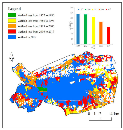
Figure 3.
Historical trajectories of wetlands from 1977 to 2017.
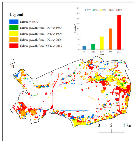
Figure 4.
Historical trajectories of urban extent from 1977 to 2017.
The wetland area and urban extent presented a spatially intersecting shift in distribution. Except for the low hills located mainly in the northern part, but partly in the southeastern part of the study area, wetlands were widely distributed in the entire region in 1977. The ranges of wetland and urban changes were limited for the period of 1977–1986. Then, urbanization expanded rapidly from the southern and northeastern parts of the study area in 1986–1993. For the next period of 1993–2006, urbanization increased continuously at the edge of the original urban areas and spread to new areas in the northwest and southwest. From 2006 to 2017, new urban area expanded significantly, not only near the original urban areas, but also around newly built roads. Meanwhile, larger areas of wetland loss were distributed in the southern and eastern edges of the Tonghu Wetland. With continuous urban growth all around the study area through the past few decades, the wetlands shrunk and became concentrated in the surroundings of Tonghu Lake.
To quantify the impact of surface hydrology on the wetland distribution from the TVWSUE methodology, the historical natural wetlands and Tonghu were mapped from 1965 to 2017 using the topographic maps and remote sensing interpretation results (Figure 5). In particular, because a project of agricultural reclamation from natural wetlands was launched in the study area in 1966, there was large-scale natural wetlands loss from 1965 to 1977. The natural shape of Tonghu Lake in 1965 had been transformed to a rectangular shape in 1977. The natural wetland area decreased significantly from 20.55 km2 to 7.96 km2 from 1965 to 1977, and the total river length decreased significantly from 195.45 km to 112.11 km. Up to 2017, the area of natural wetlands had decreased to 4.10 km2, with a change rate of more than 50%, and only the tributaries flowing into and out of Tonghu Lake were not converted to other land-use types. Most of the natural wetlands were converted to artificial wetlands, including ponds and paddy fields. Then, they were gradually converted to urbanization and other non-wetland types. The dramatic loss of rivers and small lakes, and the change of shape of Tonghu Lake, reflecting the extent of the human disturbance, influenced the regional surface hydrology and wetland distribution.
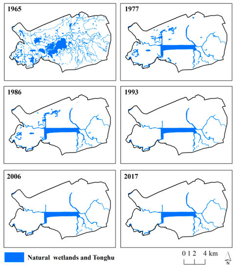
Figure 5.
Spatial distribution of natural wetlands and Tonghu in 1965, 1977, 1986, 1993, 2006, and 2017.
3.2. Relationship between Wetland Distribution and Explanatory Variables
The wetland shrinkage projection module of the TVWSUE methodology simulated the occurrence probabilities of wetlands by logistic regression models at 1977, 1986, 1993, 2006, and 2017. Using the forward stepwise strategy to select the coefficients of driving factors at the significance level of 0.05, the time-varying logistic regression models were constructed from Equation (3) (Table 5). Several variables were excluded by the statistical test, mainly climatological and topographical factors. This may be attributed to the similar spatial distribution of these variables within the small area of Tonghu Wetland, which resulted in their low impact on the wetland distribution.
Table 5.
Estimates in logistic regression of explanatory variables for predicting wetlands.
The time-varying logistic regression model and its parameters explored the relationship between wetland distribution and explanatory variables (Table 5). A positive value of β means that an increase in the particular explanatory variable increases the wetland probability. A negative value means that the variable decreases the probability of wetland. Positive values of variables of influence of urban expansion indicated that being far from the urban extent aided wetland conservation. Otherwise, wetlands near the urban extent had high loss probabilities. This is consistent with the visual result in the historical trajectories of wetland area and urban extent, in which large areas of lost wetland were occupied by urban uses or were near the urban extent (Figure 3 and Figure 4). In addition, the positive coefficient of wetland extent at the original time confirmed its impact on the future wetland distribution. The NWT was related to the regional surface hydrological linkage and confluence range, and further influenced the water supply of wetland and its occurrence probability. Thus, the negative values indicated that wetland loss occurred easily far from the NWT.
The odds ratio is a measure of the relative importance of the explanatory variables (Table 5). For β > 0, a larger odds ratio indicates a larger importance of the particular explanatory variable; for β < 0, a smaller value indicates a larger importance [63]. The increase in the odds ratio for the new urban extent variable through the four periods, with values of 1.41, 32.10, 44.39, and 183.64 for the models for 1986, 1993, 2006, and 2017, respectively, indicates an enhancing importance of urban expansion for wetland distribution. The relatively low odds ratio of urban extent at the initial time indicated a relatively low importance compared with the impact of new urban expansion on the wetland distribution. In contrast, the decrease in the odds ratio for the wetland extent variable indicated its reduced importance. The odds ratios of wetland extent were the largest for the models for 1986 and 1993, indicating a larger impact of surface hydrology for these periods. In particular, the importance of NWT remained stable at the different periods, and the importance of NWT for 1965 was relatively large, reflecting the impact of the original natural surface hydrology and geomorphology on the wetland distribution.
3.3. Performance of the TVWSUE Methodology
The urban expansion forecast module was executed to calibrate the five parameters of dispersion, breed, spread, slope resistance, and road gravity, which were determined by the values of 24, 48, 79, 21, and 35, respectively. Comparing the visually interpreted and simulated urban extent in 2017, the modified Lee and Sallee metrics had a value of 0.68. This validated the global spatial fitness of the urban expansion simulation result, on which the forecast of future expansion of urbanization in this study relied.
Statistical tests and visual comparisons were used to assess the performance of the wetland modeling. Time-varying logistic regression models were constructed in the TVWSUE methodology to predict wetland probabilities. The ROCs of the logistic regression models for 1986, 1993, 2006, and 2017 were 0.94, 0.93, 0.90, and 0.94, respectively (Table 5). The values of the ROCs, which were close to 1, confirmed the high fitness and robustness of our regression models. Meanwhile, the spatial distribution probabilities of wetlands from the regression models were mapped and compared with the visually interpreted results as a reference (Figure 6). The simulated probabilities ranged from 0 to 1, with a higher value indicating a higher likelihood of wetlands. Then, the probabilities were reclassified into five levels: very low (0–0.2), low (0.2–0.4), medium (0.4–0.6), high (0.6–0.8), and very high (0.8–1.0). On the basis of the visual assessment, most of the actually preserved wetlands were located in the areas with very high occurrence probability (Figure 6). Additionally, the occurrence probabilities of preserved wetlands and those of lost wetlands were compared. The average probabilities of preserved wetlands for 1986, 1993, 2006, and 2017 were 0.95, 0.90, 0.84, and 0.80, respectively. In contrast, the mean values of lost wetlands at the four time nodes were 0.85, 0.62, 0.56, and 0.47, respectively. The high spatial fitness of the statistical test and the visual comparison between our simulated probabilities and the referenced maps validated the effectiveness of our methodology. Except for the wetlands at 1986, which were characterized by limited wetland loss and complex driving factors, the majority of wetlands exhibited high probability values.
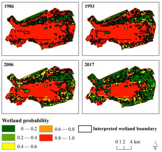
Figure 6.
Predicted wetland probabilities and preserved wetland distributions at 1986, 1993, 2006, and 2017.
The higher predicted risks of wetland loss, with low probabilities, were mainly located in or near the urban areas, particularly the new urban sprawl areas, validating the impact of urban expansion (Figure 6). To evaluate the reliability of the wetland probabilities, numbers for the five probability levels of wetlands at the initial time and the actual lost wetlands from the initial time to next time were determined. The proportion of lost wetland area to the entire area of wetlands at the different levels was calculated to evaluate the correlation between the simulated wetland probabilities and actual wetland loss (Table 6). More than 75% of the wetlands with probabilities of 0–0.2 exhibited actual loss in the periods of 1986–1993, 1993–2006, and 2006–2017, and nearly 70% with probabilities of 0.2–0.4 had actual loss at these periods. The area proportion with probabilities of 0.4–0.6 ranged from 40% to 50% at the four periods, denoting a relatively medium risk of wetland loss. Additionally, only nearly 20% and less than 10% of those areas with probabilities of 0.6–0.8 and 0.8–1.0 had actual loss during these periods. It is evident that a lower predicted probability of wetland indicates a higher risk for wetland to be actually lost under urban expansion. This result demonstrated that the probabilities of wetland occurrence calculated by our TVWSUE methodology could effectively predict the spatial distribution of future wetlands and the potential loss.
Table 6.
Actual percentages of wetland loss for various predicted probabilities of wetlands from 1977 to 2017.
To examine the impact of the time-varying variables, ROCs of logistic regression models for predicting wetlands were compared between the model with the complete variables, the model without the variable of natural wetland and Tonghu, the model without the variable of new urban extent, and the model without both of the above time-varying variables (Figure 7). The highest ROC values in our TVWSUE methodology were achieved for the model with the complete variables, which validated the necessity and effectiveness of including time-varying variables. A larger decrease in ROC for the model without the variable of new urban extent implied that this variable played a greater key role in improving model fitness than the variable of natural wetland and Tonghu. Because of the increase of the importance of the urban expansion on wetland shrinkage with increasing time (Table 5), the new urban extent variable was more important for realizing higher explanatory power in the regression model for 2017 than in that for 2006. Thus, the ROC of models with the new urban extent variable increased from 2006 to 2017. In contrast, the ROC of models without the variable decreased between these two time nodes. In particular, the average probability of actual lost wetlands at 2006–2017 for the complete logistic regression model was 0.43, which is much lower than the 0.64 for the regression model without the new urban extent variable. The absence of new urban expansion in the model significantly weakened its ability to forecast potential wetland loss.
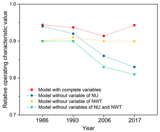
Figure 7.
Statistical comparison between logistic regression models with different explanatory variable combinations. NU: new urban extent, NWT: natural wetland and Tonghu.
3.4. Modeling of Wetland Shrinkage and Urban Expansion at Year 2030
Under the historical trend scenario, the urban extent of the Tonghu Wetland in 2030 was simulated by the urban expansion forecast module (Figure 8a). The urban area is forecast to increase from 33.60 km2 in 2017 to 47.69 km2 in 2030. With the high value of the spread parameter, the urban extent would grow outward from the existing and consolidated urban areas. In addition, a relatively high breed parameter simulated several new detached urban settlements, and the value of road gravity, ranking third among the five parameters, indicated a medium impact of the transportation network on the urban expansion, particularly, the newly built road west of Tonghu Lake. Thus, the urban extent of the Tonghu Wetland showed continuing growth, with most of the new urban areas around the urban extent in 2017 and larger expansion areas located south and northeast of the study area.

Figure 8.
Scenario maps by the TVWSUE methodology at year 2030 for (a) urban extent under the historical trend scenario, (b) wetland under the historical trend scenario, (c) urban extent under the wetland conservation scenario, and (d) wetland under the wetland conservation scenario.
With the historical trend scenario of urban growth from 2017 to 2030, using the parameters of the logistic regression model for 2017 (Table 5), the data of the time-varying explanatory variables, including the urban and wetland extent at 2017 and the new urban extent from 2017 to 2030, were updated. Then, the spatial distribution of wetland probabilities at 2030 was simulated by the TVWSUE methodology under the historical trend scenario (Figure 8b). The average value of wetland probabilities in the entire study area decreased continuously from 0.44 at 2017 to 0.34 at 2030, indicating an increasing threat of urban growth and a decreasing probability for wetland conservation in the future. In particular, the future probabilities of preserved wetlands from 2017 were identified at five levels, and the area proportions of very low (0–0.2), low (0.2–0.4), medium (0.4–0.6), high (0.6–0.8), and very high (0.8–1.0) probability were 2.36%, 6.14%, 19.57%, 20.83%, and 51.10%, respectively. The urban expansion extent from 2017 to 2030 directly occupied 7.61 km2 of the wetlands in 2017, which accounted for 11.65% of the total wetland area for 2017. Except for the direct conversion, the urban growth threatened the wetlands around the urban extent by the neighbor effect with enhanced anthropogenic disturbance intensity. Water drainage for domestic consumption, decreases in hydrological linkages between wetlands, biological invasions that modify or destroy wetlands, and living and industrial pollutants to wetlands, which tend to aggregate around urban centers, can easily cause wetland degradation and further loss [64,65]. There is still 3.06 km2 of areas with wetland probabilities <0.4, meaning a high loss likelihood from 2017 to 2030, and 8.17 km2 of areas with wetland probabilities of 0.4–0.6, denoting a medium loss likelihood. With the spatial analysis techniques, an area of 19.14 km2 of wetlands, accounting for 29.30% of the total wetland area for 2017, is under risk of loss and calls for specific conservation measures.
To protect the wetlands, a purposeful urban development and wetland protection strategy was designed based on the historical trend scenario. Areas converted from wetland areas to urban areas for 2017–2030 were labeled as excluded regions in the urban expansion forecast, and the spatial distribution of wetland probabilities for 2030 was simulated. This scenario was labeled as the “wetland conservation scenario”. Under this scenario, the area of urbanization was 40.07 km2, showing an increase of 6.47 km2 from 2017 to 2030 (Figure 8c), half of the value obtained under the historical trend scenario. With the diminished scope of urban growth, the average value of wetland probabilities under this scenario was 0.39 (Figure 8d), which is higher than the value of 0.34 under the historical trend scenario. Compared with the historical trend scenario, the area proportions of preserved wetlands from 2017 at the probabilities of 0–0.2, 0.2–0.4, and 0.4–0.6 decreased, with values of 1.08%, 2.16%, and 9.88%, respectively, and the area proportions at the probabilities of 0.6–0.8 and 0.8–1.0 increased, with values of 21.01% and 65.87%, respectively. In total, the area of wetlands under the risk of loss was 8.46 km2, which was no more than half the value under the historical scenario. Thus, the spatially specific protection strategy not only prevented urban expansion from occupying wetlands, but also relieved the neighbor-effect pressure on the wetlands. These two different scenario simulations of wetland shrinkage and urban expansion support purposeful decision-making pertaining to the tradeoff between urban growth and wetland conservation.
4. Discussion
Previous studies realized the impact of each dynamic, but studied them almost separately [3,27,28,59,66]. There is a limitation to the insights obtainable regarding the intersection of urban and wetland dynamics. The novelty of this study was the development of the TVWSUE methodology of coupling the urban expansion and wetland shrinkage processes to obtain a better approximation of wetland dynamics. Time-varying explanatory variables, including surface hydrology and urban expansion, were quantified in the model to help improve the dynamic model performance and realize future forecasting ability. Time series of the natural wetlands and Tonghu detected the influence of the original surface hydraulic linkages and geomorphology characteristics on the wetland distribution [23], which were identified by the historical change detection module of the TVWSUE methodology. Unlike the static models of previous studies, which assumed a constant influence of human activity [26,27,28,29], our time-varying regression model dynamically simulated wetland loss under the impact of urban expansion. Thus, the TVWSUE performed much better in its forecasting ability of wetland loss, showing good spatial consistency between simulated wetland probabilities and actual wetland loss (Figure 6 and Table 6). The ROC value of the TVWSUE with the time-varying variable of new urban extent was higher than that of previous models without this factor (Figure 7). Moreover, the improvement in the TVWSUE in simulating future wetland loss compared with previous static models provided more reliable information to support spatially specific wetland conservation planning.
The logistic regression model revealed the contribution importance of each explanatory variable, which indicated an increasing impact of urban expansion on the wetland distribution from 1977 to 2017 (Table 5). The human population continued to aggregate in urban centers, and urban expansion presented an inevitable increased impact on wetland loss [67], which was confirmed by the simultaneous shift between urban expansion and wetland shrinkage in the Tonghu Wetland (Figure 3 and Figure 4). With the intense human disturbance and neighbor effect of urbanization, wetlands near urban areas were also predicted to have low wetland probabilities, and these areas suffered considerable losses according to the historical changes in wetlands (Figure 6). Thus, the time-varying strategy of simultaneously simulating urban expansion and wetland shrinkage in the TVWSUE improved the model fit.
Some limitations of the TVWSUE methodology require attention. First, visually interpreting remote sensing images was time-consuming, and there were still some local interpretation errors in this study. Second, the model did not perform well in some areas, where significant actual wetland loss occurred despite relatively high predicted probability. The wetland change was driven by multiple factors that were not quantified fully in this study. In particular, complex and spatially heterogenetic human disturbances were denoted by the proximity of urban extent, which has been validated as a good proxy of human activity and successfully applied in different field studies [68,69,70]. Third, future climate change was not included in our model, in which climate variables have a non-significant impact on the wetlands in Tonghu Wetland, because of the abundant rainfall as well as the spatial homogeneity within a small area.
According to these limitations, the following improvements were suggested to be explored in a future study. A first idea is to apply multiple sources of remote sensing images [71] and cost-effective and high-accuracy mapping techniques [72]. For example, the Google Earth Engine [73] provided a big data cloud computing platform for remote sensing interpretation for data preparation and model execution of TVWSUE. The second improvement is to characterize the detailed human activities near the urban centers, which helps to increase the explanatory ability and predictive power of the TVWSUE methodology. Aside from the direct conversion from wetland to urban use, these neighbor effects of human activities played an important role in wetland shrinkage. Multiple types of data and techniques could be tested, for example, mobile phone trajectory technology [74] and street view map mining techniques [75]. The third idea is to couple different climate change scenarios [76,77] with the TVWSUE methodology. Our model is flexible in incorporating multiple explanatory variables to predict wetland probability. In addition, the combined effect of climate change and urban expansion on wetland change could be investigated.
The resulting maps in this study provided interesting tools for displaying the spatial differences of the future wetland occurrence probabilities and loss risks among different scenario designs (Figure 8) to support decision-making. Wetlands with low probabilities in the future scenario were made the focus of wetland conservation planning. Next, the scenario simulation presented the different scopes and intensities of future conflicts between urban growth and wetland protection under different management priorities and strategies (Figure 8). Under the scenario settings, the intersecting processes of urban and wetland dynamics were simulated to investigate the effects of purposeful wetland conservation policy. The exclusion method was used to place constraints on urban growth [78] and to design management scenarios, providing information useful for specific wetland conservation strategies [79]. The spatial range of the excluded layer and the weighting values placed on the suitability of cells for urban growth [78,80] can be designed to alter the urban growth pattern and examine its influence on wetland distribution. With scenario design and its interactive procedure, the TVWSUE methodology provides support for the tradeoff decision-making between urban development and wetland conservation.
5. Conclusions
Modeling wetland distribution and forecasting potential loss of wetlands can be useful for exploring the driving mechanisms of wetland shrinkage and examining the effects of different priorities and policies of urban development and wetland conservation to support tradeoff decision-making. The TVWSUE methodology, consisting of three modules, was developed in this study, which dynamically predicted wetland distribution probabilities intersecting with urban expansion by a time-varying logistic regression model. The historical change detection module revealed the intensifying conflict between wetland and urban areas from 1977 to 2017, with the proportion of wetland area decreasing from 72.16% to 43.87% and the proportion of urban extent increasing from 2.55% to 22.32%. Most of the wetland loss was located in or near the areas of urbanization. Urban areas expanded from the edge of the study area, while wetlands shrunk and were concentrated in the areas surrounding Tonghu Lake. Within the time-varying regression model, the odds ratio of the new urban extent variable increased from 1.41 in 1986 to 183.64 in 2017, indicating the increased importance of urban expansion. The modified Lee and Sallee metric of 0.68 and the ROCs greater than 0.9 for the logistic regression models validated the simulation fitness of the urban and wetland extents, respectively. Moreover, the visual consistency between our simulated and referenced wetland maps further demonstrated the effectiveness of TVWSUE. Compared with traditional methods, the incorporation of time-varying variables helped improve the model performance, with higher ROC and better ability to predict potential wetland loss. In particular, lower simulated probabilities on the wetlands were proven to indicate a higher risk of actual loss. Historical trend and wetland conservation scenarios forecasted different wetland distribution probabilities under different urban growth patterns for 2030. The historical trend scenario predicted that nearly 30% of the wetlands would be under the risk of loss in the future. With the specific exclusion strategy of urban development, areas of wetland loss risk were decreased by more than 50% in the wetland conservation scenario. The scenario designs and the interactive procedures of the methodology were able to provide information on the intersecting processes of future urban expansion and wetland shrinkage useful for informing a spatially specific wetland conservation strategy. Our results validated the effectiveness of the TVWSUE methodology and the significance of tradeoff decision-making between urban development and wetland conservation. The aforementioned limitations and improvements of the TVWSUE methodology were suggested for testing in future studies.
Author Contributions
E.X. and Y.C. conceived and designed the experiments. E.X. analyzed the data. E.X. and Y.C. wrote and revised the paper.
Funding
This work was financially supported by National Natural Science Foundation of China (Grant No. 41601095), Strategic Priority Research Program of the Chinese Academy of Sciences (XDA19040305), Huizhou’s Science and Technology Special Fund Project (2016X0436051), and Provincial Key Education-Specialty Innovation Research Project of Guangdong (2018KTSCX216).
Conflicts of Interest
The authors declare no conflict of interest.
References
- Zedler, J.B.; Kercher, S. Wetland resources: Status, trends, ecosystem services, and restorability. Annu. Rev. Environ. Resour. 2005, 30, 39–74. [Google Scholar] [CrossRef]
- Sica, Y.V.; Quintana, R.D.; Radeloff, V.; Gavier-Pizarro, G. Wetland loss due to land use change in the Lower Paraná River Delta, Argentina. Sci. Total Environ. 2016, 568, 967–978. [Google Scholar] [CrossRef] [PubMed]
- Mondal, B.; Dolui, G.; Pramanik, M.; Maity, S.; Biswas, S.S.; Pal, R. Urban expansion and wetland shrinkage estimation using a GIS-based model in the East Kolkata Wetland, India. Ecol. Indic. 2017, 83, 62–73. [Google Scholar] [CrossRef]
- Gardner, R.C.; Barchiesi, S.; Beltrame, C.; Finlayson, C.; Galewski, T.; Harrison, I.; Paganini, M.; Perennou, C.; Pritchard, D.; Rosenqvist, A. State of the world’s wetlands and their services to people: A compilation of recent analyses. SRN Electron. J. 2015. [Google Scholar] [CrossRef]
- Gibbs, J.P. Wetland loss and biodiversity conservation. Conserv. Biol. 2000, 14, 314–317. [Google Scholar] [CrossRef]
- Hategekimana, S.; Twarabamenya, E. The impact of wetlands degradation on water resources management in Rwanda: The case of Rugezi Marsh. In Proceedings of the 5th International Symposium on Hydrology, Cario, Egypt, 2007. [Google Scholar]
- An, S.; Wang, Z.; Zhou, C.; Guan, B.; Deng, Z.; Zhi, Y.; Liu, Y.; Xu, C.; Fang, S.; Xu, Z. The headwater loss of the western plateau exacerbates China’s long thirst. AMBIO J. Hum. Environ. 2006, 35, 271–273. [Google Scholar] [CrossRef] [PubMed]
- Gulbin, S.; Kirilenko, A.P.; Kharel, G.; Zhang, X. Wetland loss impact on long term flood risks in a closed watershed. Environ. Sci. Policy 2019, 94, 112–122. [Google Scholar] [CrossRef]
- Mitsch, W.J.; Bernal, B.; Hernandez, M.E. Ecosystem services of wetlands. Int. J. Biodivers. Sci. Ecosyst. Serv. Manag. 2015, 11, 1–4. [Google Scholar] [CrossRef]
- Quesnelle, P.E.; Fahrig, L.; Lindsay, K.E. Effects of habitat loss, habitat configuration and matrix composition on declining wetland species. Biol. Conserv. 2013, 160, 200–208. [Google Scholar] [CrossRef]
- Nicholls, R.J. Coastal flooding and wetland loss in the 21st century: Changes under the SRES climate and socio-economic scenarios. Glob. Environ. Chang. 2004, 14, 69–86. [Google Scholar] [CrossRef]
- Robertson, L.D.; King, D.J.; Davies, C. Assessing land cover change and anthropogenic disturbance in wetlands using vegetation fractions derived from Landsat 5 TM imagery (1984–2010). Wetlands 2015, 35, 1077–1091. [Google Scholar] [CrossRef]
- Verburg, P.H.; Schot, P.P.; Dijst, M.J.; Veldkamp, A. Land use change modelling: Current practice and research priorities. GeoJournal 2004, 61, 309–324. [Google Scholar] [CrossRef]
- Van Schrojenstein Lantman, J.; Verburg, P.H.; Bregt, A.; Geertman, S. Core principles and concepts in land-use modelling: A literature review. In Land-Use Modelling in Planning Practice; Springer: Dordrecht, The Netherlands, 2011; pp. 35–57. [Google Scholar]
- Santé, I.; García, A.M.; Miranda, D.; Crecente, R. Cellular automata models for the simulation of real-world urban processes: A review and analysis. Landsc. Urban Plan. 2010, 96, 108–122. [Google Scholar] [CrossRef]
- De Rosa, M.; Knudsen, M.T.; Hermansen, J.E. A comparison of Land Use Change models: Challenges and future developments. J. Clean. Prod. 2016, 113, 183–193. [Google Scholar] [CrossRef]
- Brown, D.G.; Verburg, P.H.; Pontius, R.G.; Lange, M.D. Opportunities to improve impact, integration, and evaluation of land change models. Curr. Opin. Environ. Sustain. 2013, 5, 452–457. [Google Scholar] [CrossRef]
- Matthews, R.B.; Gilbert, N.G.; Roach, A.; Polhill, J.G.; Gotts, N.M. Agent-based land-use models: A review of applications. Landsc. Ecol. 2007, 22, 1447–1459. [Google Scholar] [CrossRef]
- Verburg, P.H.; Soepboer, W.; Veldkamp, A.; Limpiada, R.; Espaldon, V.; Mastura, S.S. Modeling the spatial dynamics of regional land use: The CLUE-S model. Environ. Manag. 2002, 30, 391–405. [Google Scholar] [CrossRef] [PubMed]
- Verburg, P.H.; Overmars, K.P. Combining top-down and bottom-up dynamics in land use modeling: Exploring the future of abandoned farmlands in Europe with the Dyna-CLUE model. Landsc. Ecol. 2009, 24, 1167. [Google Scholar] [CrossRef]
- Van Asselen, S.; Verburg, P.H. Land cover change or land-use intensification: Simulating land system change with a global-scale land change model. Glob. Chang. Biol. 2013, 19, 3648–3667. [Google Scholar] [CrossRef]
- Groeneveld, J.; Müller, B.; Buchmann, C.M.; Dressler, G.; Guo, C.; Hase, N.; Hoffmann, F.; John, F.; Klassert, C.; Lauf, T. Theoretical foundations of human decision-making in agent-based land use models–A review. Environ. Model. Softw. 2017, 87, 39–48. [Google Scholar] [CrossRef]
- Sánchez-González, S.; Martínez-Alegría, R.; Taboada, J. Modeling wetland change in Spain’s Tierra de Campos district. Wetl. Ecol. Manag. 2016, 24, 399–410. [Google Scholar] [CrossRef]
- Jamru, L.R.; Rahaman, Z.A. Combination of spatial logistic regression and geographical information systems in modelling wetland changes in Setiu basin, Terengganu. In IOP Conference Series: Earth and Environmental Science; IOP Publishing: Bristol, UK, 2018; p. 012106. [Google Scholar]
- Cui, L.; Gao, C.; Zhou, D.; Mu, L. Quantitative analysis of the driving forces causing declines in marsh wetland landscapes in the Honghe region, northeast China, from 1975 to 2006. Environ. Earth Sci. 2014, 71, 1357–1367. [Google Scholar] [CrossRef]
- Koneff, M.D.; Royle, J.A. Modeling wetland change along the United States Atlantic Coast. Ecol. Model. 2004, 177, 41–59. [Google Scholar] [CrossRef]
- Chen, H.; Zhang, W.; Gao, H.; Nie, N. Climate change and anthropogenic impacts on wetland and agriculture in the Songnen and Sanjiang Plain, northeast China. Remote Sens. 2018, 10, 356. [Google Scholar] [CrossRef]
- Liu, H.; Bu, R.; Liu, J.; Leng, W.; Hu, Y.; Yang, L.; Liu, H. Predicting the wetland distributions under climate warming in the Great Xing’an Mountains, northeastern China. Ecol. Res. 2011, 26, 605–613. [Google Scholar] [CrossRef]
- Zhao, D.; He, H.; Wang, W.; Wang, L.; Du, H.; Liu, K.; Zong, S. Predicting Wetland Distribution Changes under Climate Change and Human Activities in a Mid-and High-Latitude Region. Sustainability 2018, 10, 863. [Google Scholar] [CrossRef]
- Akin, A.; Berberoğlu, S.; Erdogan, M.A.; Donmez, C. Modelling land-use change dynamics in a Mediterranean coastal wetland using CA-Markov chain analysis. Fresenius Environ. Bull. 2012, 21, 386–396. [Google Scholar]
- Yu, H.; He, Z.; Pan, X. Wetlands shrink simulation using cellular automata: A case study in Sanjiang Plain, China. Procedia Environ. Sci. 2010, 2, 225–233. [Google Scholar] [CrossRef]
- Wang, H.; He, Q.; Liu, X.; Zhuang, Y.; Hong, S. Global urbanization research from 1991 to 2009: A systematic research review. Landsc. Urban Plan. 2012, 104, 299–309. [Google Scholar] [CrossRef]
- Rojas, C.; Munizaga, J.; Rojas, O.; Martínez, C.; Pino, J. Urban development versus wetland loss in a coastal Latin American city: Lessons for sustainable land use planning. Land Use Policy 2019, 80, 47–56. [Google Scholar] [CrossRef]
- Grimmond, S.U.E. Urbanization and global environmental change: Local effects of urban warming. Geogr. J. 2007, 173, 83–88. [Google Scholar] [CrossRef]
- Ahn, C.; Schmidt, S. Designing Wetlands as an Essential Infrastructural Element for Urban Development in the era of Climate Change. Sustainability 2019, 11, 1920. [Google Scholar] [CrossRef]
- Aburas, M.M.; Ho, Y.M.; Ramli, M.F.; Ash’aari, Z.H. The simulation and prediction of spatio-temporal urban growth trends using cellular automata models: A review. Int. J. Appl. Earth Obs. Geoinf. 2016, 52, 380–389. [Google Scholar] [CrossRef]
- Clarke, K.C.; Hoppen, S.; Gaydos, L. A self-modifying cellular automaton model of historical urbanization in the San Francisco Bay area. Environ. Plan. B Plan. Des. 1997, 24, 247–261. [Google Scholar] [CrossRef]
- Triantakonstantis, D.; Mountrakis, G. Urban growth prediction: A review of computational models and human perceptions. J. Geogr. Inf. Syst. 2012, 4, 555. [Google Scholar] [CrossRef]
- Chaudhuri, G.; Clarke, K. The SLEUTH land use change model: A review. Environ. Resour. Res. 2013, 1, 88–105. [Google Scholar]
- Haas, J.; Ban, Y. Urban growth and environmental impacts in Jing-Jin-Ji, the Yangtze, River Delta and the Pearl River Delta. Int. J. Appl. Earth Obs. Geoinf. 2014, 30, 42–55. [Google Scholar] [CrossRef]
- Wang, Y.; Gao, J.; Liu, Z. Pollution Load and Environment Capacity in Tonghu Lake Basin. Wetland Sci. 2016, 14, 354–360, (In Chinese with English Abstract). [Google Scholar]
- Li, D. Thoughts on water conservancy construction and wetland protection in tonghu area. Guangdong Water Resour. Hydropower 2011, 8, 15–17, (In Chinese with English Abstract). [Google Scholar]
- Deng, X.; Huang, J.; Rozelle, S.; Uchida, E. Growth, population and industrialization, and urban land expansion of China. J. Urban Econ. 2008, 63, 96–115. [Google Scholar] [CrossRef]
- Matthews, G.V.T. The Ramsar Convention on Wetlands: Its History and Development; Ramsar Convention Bureau: Gland, Switzerland, 1993. [Google Scholar]
- Liu, G.; Zhang, L.; Zhang, Q.; Musyimi, Z.; Jiang, Q. Spatio–Temporal Dynamics of Wetland Landscape Patterns Based on Remote Sensing in Yellow River Delta, China. Wetlands 2014, 34, 787–801. [Google Scholar] [CrossRef]
- Li, X.; Xue, Z.; Gao, J. Dynamic changes of plateau wetlands in Madou County, the Yellow River source zone of China: 1990–2013. Wetlands 2016, 36, 299–310. [Google Scholar] [CrossRef]
- Jiyuan, L.; Mingliang, L.; Xiangzheng, D.; Dafang, Z.; Zengxiang, Z.; Di, L. The land use and land cover change database and its relative studies in China. J. Geogr. Sci. 2002, 12, 275–282. [Google Scholar] [CrossRef]
- Davranche, A.; Lefebvre, G.; Poulin, B. Wetland monitoring using classification trees and SPOT-5 seasonal time series. Remote Sens. Environ. 2010, 114, 552–562. [Google Scholar] [CrossRef]
- Landmann, T.; Schramm, M.; Colditz, R.R.; Dietz, A.; Dech, S. Wide area wetland mapping in semi-arid Africa using 250-meter MODIS metrics and topographic variables. Remote Sens. 2010, 2, 1751–1766. [Google Scholar] [CrossRef]
- Phiri, D.; Morgenroth, J. Developments in Landsat Land Cover Classification Methods: A Review. Remote Sens. 2017, 9, 967. [Google Scholar] [CrossRef]
- Tu, M.-C.; Smith, P.; Filippi, A.M. Hybrid forward-selection method-based water-quality estimation via combining Landsat TM, ETM+, and OLI/TIRS images and ancillary environmental data. PLoS ONE 2018, 13, e0201255. [Google Scholar] [CrossRef] [PubMed]
- Kindu, M.; Schneider, T.; Teketay, D.; Knoke, T. Land Use/Land Cover Change Analysis Using Object-Based Classification Approach in Munessa-Shashemene Landscape of the Ethiopian Highlands. Remote Sens. 2013, 5, 2411–2435. [Google Scholar] [CrossRef]
- Dessie, G.; Kleman, J. Pattern and Magnitude of Deforestation in the South Central Rift Valley Region of Ethiopia. Mt. Res. Dev. 2007, 27, 162–168. [Google Scholar] [CrossRef]
- Lobo, F.L.; Costa, M.P.F.; Novo, E.M.L.M. Time-series analysis of Landsat-MSS/TM/OLI images over Amazonian waters impacted by gold mining activities. Remote Sens. Environ. 2015, 157, 170–184. [Google Scholar] [CrossRef]
- Vitousek, P.M.; Mooney, H.A.; Lubchenco, J.; Melillo, J.M. Human domination of Earth’s ecosystems. Science 1997, 277, 494–499. [Google Scholar] [CrossRef]
- Silva, E.A.; Clarke, K.C. Calibration of the SLEUTH urban growth model for Lisbon and Porto, Portugal. Comput. Environ. Urban Syst. 2002, 26, 525–552. [Google Scholar] [CrossRef]
- Rienow, A.; Goetzke, R. Supporting SLEUTH–Enhancing a cellular automaton with support vector machines for urban growth modeling. Comput. Environ. Urban Syst. 2015, 49, 66–81. [Google Scholar] [CrossRef]
- Oguz, H.; Klein, A.; Srinivasan, R. Using the SLEUTH urban growth model to simulate the impacts of future policy scenarios on urban land use in the Houston-Galveston-Brazoria CMSA. Res. J. Soc. Sci. 2007, 2, 72–82. [Google Scholar]
- Bihamta, N.; Soffianian, A.; Fakheran, S.; Gholamalifard, M. Using the SLEUTH urban growth model to simulate future urban expansion of the Isfahan metropolitan area, Iran. J. Indian Soc. Remote Sens. 2015, 43, 407–414. [Google Scholar] [CrossRef]
- Dietzel, C.; Clarke, K.C. Spatial differences in multi-resolution urban automata modeling. Trans. GIS 2004, 8, 479–492. [Google Scholar] [CrossRef]
- Yang, X.; Lo, C.P. Using a time series of satellite imagery to detect land use and land cover changes in the Atlanta, Georgia metropolitan area. Int. J. Remote Sens. 2002, 23, 1775–1798. [Google Scholar] [CrossRef]
- Greiner, M.; Pfeiffer, D.; Smith, R. Principles and practical application of the receiver-operating characteristic analysis for diagnostic tests. Prev. Vet. Med. 2000, 45, 23–41. [Google Scholar] [CrossRef]
- Peduzzi, P.; Concato, J.; Kemper, E.; Holford, T.R.; Feinstein, A.R. A simulation study of the number of events per variable in logistic regression analysis. J. Clin. Epidemiol. 1996, 49, 1373–1379. [Google Scholar] [CrossRef]
- Johnston, C.A. Wetland losses due to row crop expansion in the Dakota Prairie Pothole Region. Wetlands 2013, 33, 175–182. [Google Scholar] [CrossRef]
- Lee, S.; Dunn, R.; Young, R.; Connolly, R.; Dale, P.; Dehayr, R.; Lemckert, C.; McKinnon, S.; Powell, B.; Teasdale, P. Impact of urbanization on coastal wetland structure and function. Austral Ecol. 2006, 31, 149–163. [Google Scholar] [CrossRef]
- Hua, L.; Tang, L.; Cui, S.; Yin, K. Simulating urban growth using the SLEUTH model in a coastal peri-urban district in China. Sustainability 2014, 6, 3899–3914. [Google Scholar] [CrossRef]
- Kentula, M.E.; Gwin, S.E.; Pierson, S.M. Tracking changes in wetlands with urbanization: Sixteen years of experience in Portland, Oregon, USA. Wetlands 2004, 24, 734–743. [Google Scholar] [CrossRef]
- Xu, E.; Zhang, H.; Yao, L. An Elevation-Based Stratification Model for Simulating Land Use Change. Remote Sens. 2018, 10, 1730. [Google Scholar] [CrossRef]
- Brinkmann, K.; Noromiarilanto, F.; Ratovonamana, R.Y.; Buerkert, A. Deforestation processes in south-western Madagascar over the past 40 years: What can we learn from settlement characteristics? Agric. Ecosyst. Environ. 2014, 195, 231–243. [Google Scholar] [CrossRef]
- Oberosler, V.; Groff, C.; Iemma, A.; Pedrini, P.; Rovero, F. The influence of human disturbance on occupancy and activity patterns of mammals in the Italian Alps from systematic camera trapping. Mamm. Biol. 2017, 87, 50–61. [Google Scholar] [CrossRef]
- Zhang, J. Multi-source remote sensing data fusion: Status and trends. Int. J. Image Data Fusion 2010, 1, 5–24. [Google Scholar] [CrossRef]
- Myint, S.W.; Gober, P.; Brazel, A.; Grossman-Clarke, S.; Weng, Q. Per-pixel vs. object-based classification of urban land cover extraction using high spatial resolution imagery. Remote Sens. Environ. 2011, 115, 1145–1161. [Google Scholar] [CrossRef]
- Gorelick, N.; Hancher, M.; Dixon, M.; Ilyushchenko, S.; Thau, D.; Moore, R. Google Earth Engine: Planetary-scale geospatial analysis for everyone. Remote Sens. Environ. 2017, 202, 18–27. [Google Scholar] [CrossRef]
- Vazquez-Prokopec, G.M.; Bisanzio, D.; Stoddard, S.T.; Paz-Soldan, V.; Morrison, A.C.; Elder, J.P.; Ramirez-Paredes, J.; Halsey, E.S.; Kochel, T.J.; Scott, T.W. Using GPS technology to quantify human mobility, dynamic contacts and infectious disease dynamics in a resource-poor urban environment. PLoS ONE 2013, 8, e58802. [Google Scholar] [CrossRef]
- Li, X.; Ratti, C.; Seiferling, I. Mapping urban landscapes along streets using google street view. In Proceedings of the International Cartographic Conference (ICACI 2017), Washington, DC, USA, 2–7 July 2017; pp. 341–356. [Google Scholar]
- Arnell, N.W. Climate change and global water resources: SRES emissions and socio-economic scenarios. Glob. Environ. Chang. 2004, 14, 31–52. [Google Scholar] [CrossRef]
- Nakicenovic, N.; Alcamo, J.; Grubler, A.; Riahi, K.; Roehrl, R.; Rogner, H.-H.; Victor, N. Special Report on Emissions Scenarios (SRES), a Special Report of Working Group III of the Intergovernmental Panel on Climate Change; Cambridge University Press: Cambridge, UK, 2000. [Google Scholar]
- Dietzel, C.; Clarke, K.C. Toward Optimal Calibration of the SLEUTH Land Use Change Model. Trans. GIS 2007, 11, 29–45. [Google Scholar] [CrossRef]
- Akın, A.; Clarke, K.C.; Berberoglu, S. The impact of historical exclusion on the calibration of the SLEUTH urban growth model. Int. J. Appl. Earth Obs. Geoinf. 2014, 27, 156–168. [Google Scholar] [CrossRef]
- Jantz, C.A.; Goetz, S.J.; Donato, D.; Claggett, P. Designing and implementing a regional urban modeling system using the SLEUTH cellular urban model. Comput. Environ. Urban Syst. 2010, 34, 1–16. [Google Scholar] [CrossRef]
© 2019 by the authors. Licensee MDPI, Basel, Switzerland. This article is an open access article distributed under the terms and conditions of the Creative Commons Attribution (CC BY) license (http://creativecommons.org/licenses/by/4.0/).