Quantifying Impacts of Urban Microclimate on a Building Energy Consumption—A Case Study
by
 , ,
, ,
Jiying Liu
1,2,* ,
,
Mohammad Heidarinejad
3 ,
,
Saber Khoshdel Nikkho
2,
Nicholas W. Mattise
2 and
Jelena Srebric
2 1
School of Thermal Engineering, Shandong Jianzhu University, Jinan 250101, China
2
Department of Mechanical Engineering, University of Maryland, College Park, MD 20742, USA
3
Department of Civil, Architectural, and Environmental Engineering, Illinois Institute of Technology, Chicago, IL 60616, USA
*
Author to whom correspondence should be addressed.
Sustainability 2019, 11(18), 4921; https://doi.org/10.3390/su11184921
Submission received: 31 July 2019
/
Revised: 29 August 2019
/
Accepted: 4 September 2019
/
Published: 9 September 2019
(This article belongs to the Special Issue Building and Urban Energy Prediction-Big Data Analysis and Sustainable Design)
Abstract
:This paper considered an actual neighborhood to quantify impacts of the local urban microclimate on energy consumption for an academic building in College Park, USA. Specifically, this study accounted for solar irradiances on building and ground surfaces to evaluate impacts of the local convective heat transfer coefficient (CHTC), infiltration rate, and coefficient of performance (COP) on building cooling systems. Using computational fluid dynamics (CFD) allowed for the calculation of local temperature and velocity values and implementation of the local variables in the building energy simulation (BES) model. The discrepancies among the cases with different CHTCs showed slight influence of CHTCs on sensible load, in which the maximum variations existed 1.95% for sensible cooling load and 3.82% for sensible heating load. The COP analyses indicated windward wall and upstream roof are the best locations for the installation of these cooling systems. This study used adjusted infiltration rate values that take into account the local temperature and velocity. The results indicated the annual cooling and heating energy increased by 2.67% and decreased by 2.18%, respectively.
1. Introduction
In the last two decades, numerous cities face serious problems of rapid urbanization [1,2], energy consumption [3,4,5,6,7], and climate change [8,9]. It is estimated more than 70% of people will reside in the built environment by 2050. More and more studies have been continuously demonstrated that the urban microclimate environment has a crucial impact on building energy consumption patterns [10,11]. Allegrini et al. [12] presented the importance of buoyancy for low wind speed cases in an urban environment and the strong influence of buildings upstream on the heat fluxes and temperatures further downstream. Liu et al. [13] found that the local microclimate, characterized by the exterior surface convective heat transfer coefficients (CHTCs), could affect the total cooling energy consumption by 4%. Yang et al. [14] showed that a significant cooling load reduction of 18.8% was found when considering the solar shading effect by the surrounding obstructions. A review concluded that the urban microclimate can have a net positive effect on the building energy demand on a yearly basis [15]. Existing studies typically have considered one influential variable isolated from the other influential variables, for example, CHTCs [16,17,18], wind speed [19,20], wind direction [20,21], thermal parameters [22], neighborhood densities [23], urban geometrical parameters [24,25], and solar radiation [26,27,28]. However, there are limited quantitative studies to comprehensively understand the impacts of the outdoor built environment on building energy consumption patterns. Therefore, consideration of more parameters is necessary to accurately assess the effect of the urban microclimate on building energy demand.
Moreover, in most of the urban microclimate studies, researchers usually use regular building shapes in an isolated-scale or neighborhood-scale environment [15,29]. Due to the complex and variable nature of urban microclimate environments, there are fewer researches that have considered the importance of modified variables based on the urban microclimate on simulated energy consumption in a real case. In a real urban environment, building’s surroundings create a wind sheltering and shading effect that can reduce local wind speed patterns and decrease the building surface temperatures [30,31], which become an important factor affecting building energy consumption. Literature review shows that it is crucial to account for the influence of thermo-fluid properties of air and surfaces in the local built environment on building energy consumption patterns [32]. Therefore, it is highly recommended to (i) quantify the impact of thermo-fluid variables, (ii) develop new urban-scale physical models that can account for the impact of the urban microclimate on the energy consumption patterns of buildings, and (iii) demonstrate the developed physical models on an actual urban neighborhood. Finally, this study aims to consider a combination of the thermo-fluid variables and quantify the impacts of the urban microclimate on building energy use patterns in a real academic building in College Park, USA.
2. Research Methodology
This section provided details about the description of the case study building, airflow simulation, and energy models setup, including the coupling strategy for the data exchange between different simulation engines, and local parameters in the outdoor thermal environments.
2.1. Description of the Case Study Building
The case study building, named Susquehanna North, is a four-story academic building and hosts different academic departments with about 45% office areas, 25% classrooms, 25% common areas, and 5% other spaces. The buildings gross floor area is 4968 m2 (53,478 ft2). The building uses electricity for daily electric use, heating, and cooling. There is a requirement for natural gas consumption in the early morning for days when there is a need for pre-heating the space. This consumption is minimal, thus could be ignored for the actual building consumption. In 2015, the energy utilization index of this building was 268.1 kWh/m2 (85 kBtu/ft2).
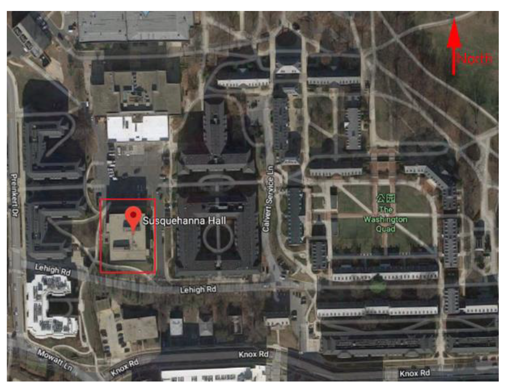
Figure 1 illustrates the selected neighborhood with the building of interest. The criteria for the selection of this case study and neighborhood are: (i) Urban plan area density, (ii) accessibility to building energy data, (iii) selecting a building with all electric energy consumption and rooftop unit, and (iv) configuration of the urban neighborhood.
2.2. CFD and Energy Models Setup
2.2.1. One-Way Coupling Strategy
This study used a one-directional coupling strategy to perform a co-simulation of the outdoor airflow computational fluid dynamics (CFD) and building energy simulation (BES). Figure 2 illustrates the simplified simulation framework suggested by this study to perform co-simulation of outdoor airflow CFD and BES. The airflow and energy processes in the urban neighborhood have different spatial and temporal scales. Therefore, to couple the solution and to enable rapid and accurate data exchange of information between different engines, there is a need to benefit from the existing coupling strategies [33].
There are different coupling strategies to account for the interaction of airflow, energy, and heat equations to couple the air properties with the exterior thermal properties of impervious and pervious surfaces [34]. When the aim of a particular study is to assess the impacts of the built environment on the indoor environment, coupling the internal properties with the change of the outdoor variable is required. This is the case for the internal coupling. However, when the focus is on the direct interaction of the outdoor and indoor environments, and more specifically the interface between the indoor and outdoor environments, there is a need to benefit from the external coupling strategies. In general, due to the current performance design practice of buildings and the insulation of the recent buildings, the internal coupling tends to be less effective.
Another consideration for the data exchange of the variables is the frequency and direction of the data exchange. The one-way coupling strategy requires exchanges of data from one set of equations to another set of equations. Other form of data exchange for rapid changes needs to use a two-way data exchange of data from the equations. Depending on the frequency of data exchange, different strategies are proposed. Quasi-steady and dynamic two-way coupling are examples of commonly recommended two-way data exchange. When the frequency of the data exchange is more frequent, there is a need to utilize the virtual environment, which allows dynamic exchange of the simulation tools. In other words, for the interactive data exchange of EnergyPlus time steps with the outdoor airflow simulations, the virtual environment program was used. However, at present, it is not possible to conduct a full-scale real-time CFD simulation due to limitations in the computational and storage capacities. Consequently, most of the integrated building energy and airflow simulations conduct a limited number of steady-state CFD airflow simulations, allowing for the assessment of building energy performance [35]. This study relied on performing CFD simulations at representative times of the year. Overall, this study used one-way coupling relying on urban-scale physical models and simulation engines, including CFD, BES, and ray-tracing radiance, for an actual urban neighborhood located at the University of Maryland College Park, to facilitate the computational time of the urban-scale simulations.
2.2.2. CFD Simulation
This study used a modified version of the OpenFOAM solver to calculate CHTC values [36]. The realizable k-ε turbulence model was modeled to compare the urban microclimate environment. The governing conservation equations for the incompressible airflow simulations are:
where and are velocity, Reynolds stress, thermal expansion, temperature, and pressure, respectively. The following equations allow one to approximate the Reynolds stress tensor:
where , and are the turbulent kinetic energy, turbulent dissipation, turbulent eddy viscosity, and a constant, respectively; the value for the constant is 0.0845. Additionally, the calculation of turbulent thermal diffusivity benefits from the thermal diffusion and the turbulent Prandtl number. For this study, Prandtl number is 0.8.
In the atmospheric boundary layer (ABL), a logarithmic wind velocity profile models the characteristic of the incoming wind. The atmBoundaryLayerInletVelocity boundary condition in OpenFOAM was implemented to represents ABL based on the following equation [37]:
where are friction velocity, elevation above the ground, elevation of the ground, roughness length of the ground, and Von Karman constant ( = 0.41), respectively. In this equation, is equal to 0.3 m; this is because there are small obstacles in the studied neighborhood. Finally, the equations for the calculation of and are [38]:
Figure 3 illustrates the CFD mesh in the three-dimensional domain, the mesh adjacent to the building of interest, and the boundary layer mesh close to the building wall. This study used blockMesh and snappyHexMesh, two meshing tools in OpenFOAM, to create the CFD mesh. Figure 3a shows that the blockMesh creates the background mesh, and Figure 3b,c shows that the snappyHexMesh establishes the domain mesh. The new solver is named buoyantBoussinesqSimpleFoamBSIM, which is similar to the original buoyantBoussinesqSimpleFoam and empowers this study to export detailed CHTC and Cp on the building and ground surfaces. Based on the OpenFOAM requirements, the entire neighborhood comprised of 15 buildings was imported as STL (STereoLithography) format in OpenFOAM.
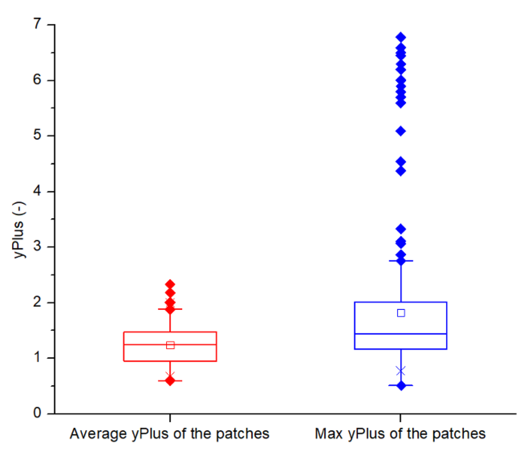
To make sure the simulation results were within the acceptable range of variation close to the building walls where most of the heat and mass transfer interactions occur, this study considered both average and maximum values of the dimensionless wall distance (y+) for the simulations. This study is one of the few studies to report the y+ variation for all of the cells close to the building walls. Figure 4 shows the y+ profiles at the centerline locations in the windward, leeward, lateral, and roof surfaces. Figure 5 illustrates all the distribution of y+ on the CFD patches next to the building surfaces. The values of the median y+ for both average and maximum were less than 10. Overall, the patches had y+ less than 10 and less than the recommended values for the y+ variation in the outdoor airflow simulations [12,20,32].
For the grid independence analysis, the grid convergence index (GCI = FS|ε|(rp−1)) was used to verify the model convergence rate [29,39], where FS = 1.25 is the safety factor when comparing three grids, ε is the velocity magnitude relative error for specified measured point between coarse and fine grid solutions, and p = 2 represents the second order method. Finally, this study used about 10 million cells for the refined mesh to reach a maximum GCI of 5%.
Figure 6 illustrates the imposed heat fluxes on the building and ground surfaces. This figure shows that solar heat fluxes reach up to 550 W/m2 at the horizontal surfaces and there are low values in the shaded areas next to the building surfaces. The inlet air temperature in the boundary condition was 30 °C, and this study modeled the solar radiation on 21 July 2014 at 12 p.m. This day was selected since it was the warmest day of summer for 2014 and can support design and sizing of heating, ventilation, and air conditioning (HVAC) equipment. The wind direction was in the south direction with a wind speed of 5 m/s at a height of 10 m. For the emissivity, uniform value of 0.90 was chosen for the ground and building walls. The residuals for this study are less than 10−4 except pressure variable that has a residual of 10−3 to 10−4.
2.2.3. Building Energy Simulation
In this study, the heat balance on the outside surface for building energy simulation in EnergyPlus follows the equation below [40]:
where , , , are the absorbed solar radiation, the estimated net longwave radiation, the net heat transfer due to the outdoor air via convection, and the heat transferred through the building envelope, respectively. The variable that is in the interest of this paper is the CHTC that is calculated as:
where , , , and are the CHTC, the fluid-solid contact area through which heat flows, the building wall surface temperatures, and the air temperatures adjacent to a building, respectively.
This study used OpenStudio to create the building energy model and implement the modified thermo-fluid properties in the EnergyPlus model. Figure 7 shows the OpenStudio model geometry. The building is all electric, and heating and cooling from this building originates from electricity. The actual building has rooftop units similar to the building energy model. The building energy model has 52 thermal zones.
Throughout the detailed calibration process, the original inputs from the U.S. Department of Energy (DOE) Reference Buildings [41] were changed based on the University of Maryland’s regulations for temperature setpoints and based on the actual building operation [42]. Table 1 provides a calibrated summary of the building energy model setup including building setpoints, operational schedules, and density loads.
2.3. Local Parameters in the Outdoor Thermal Environment
2.3.1. Local CHTCs
In the urban microclimate environment, accurate utilization of exterior CHTCs has a significant effect on the cooling energy consumption. The CHTCs not only vary at the different surface locations associated with building densities, such as the windward, leeward, and roof surfaces of a building located in an urban neighborhood, but they also vary with urban microclimate environment, such as the local wind environment and the local thermal environment. Therefore, this study used urban-scale CHTC correlations and commonly-used CHTC correlations to quantify the impact of exterior-surface CHTC correlations on the simulated energy consumption results that are directly affected by the urban microclimate.
To describe the characteristic of CHTC distribution in the building of interest, representative CHTC profiles at the centerline locations in the windward, leeward, lateral, and roof surfaces are presented as shown in Figure 8. It was found that CHTCs increased with the increase of building height for windward, leeward, and lateral surfaces, and then decreased for the leeward and lateral-east surfaces. It should be noted that the forced CHTC is proportional to the air velocity magnitude adjacent to the building wall. The flow regime has a significant effect on the CHTC distributions [21]. The flow field at the upstream building is characterized by impingement, separation, and reattachment [23]. First, the flow separates at the front corners of the windward surface resulting in a wake region in the lateral and top surfaces of the upstream building. Then, the flow attaches to the lateral and top surfaces of the downstream building. Moreover, this phenomenon was consistent with inlet velocity profile, in which the smaller velocity magnitude occured adjacent to the building surface at the bottom domain.
In addition, due to the effect of solar radiation, the CHTCs in the east wall are larger than those in west wall. In the end, Table 2 summarizes the CHTC correlations using combined local velocities (Uloc) and the temperature difference (∆T) derived from the case study building. Note that the CHTC in the windward surface is larger than the roof, which is caused by the flow field with the impingement in the upstream building, and the separation in the roof surface.
This study also used urban building densities to calculate the urban-scale CHTC correlations based on the local urban microclimate, and implements the urban-scale CHTC correlations. The derived CHTC correlations from the case study building and commonly-used CHTC correlations (DOE-2) are applied to evaluate the impacts of the CHTCs on the cooling energy consumption patterns of the selected case study. Table 3 shows the CHTC correlations’ combined Uloc and ∆T for urban-scale CHTC correlation considering the actual plan area density (λp = 0.23) [13].
2.3.2. Local Air Temperature
The outdoor air temperature can significantly influence the energy consumption, which is characterized by the coefficient of performance (COP) representing the efficiency of the cooling systems. The local microclimate could decrease COP of the cooling system up to 10% [43]. Therefore, this study used three different equations to quantify degradation in the efficiency of building cooling systems installed on the window side and rooftop. Equations (12)–(14) are the commonly-used equations to quantify COP of the cooling system based on the outdoor air temperature (). It is important to note that: (i) Equation (12) is valid for outdoor temperatures between 25 and 45 °C and room temperatures equal to 23 °C for split systems [44], (ii) Equation (13) is valid for rooftop units and is the outdoor temperature in Fahrenheit in this equation [45], and (iii) Equation (14) is applicable for room temperatures equal to 27 °C for split systems [44]. These equations are considered to emphasize the significance of urban microclimate impact on building energy consumption, accounting for different kinds of local parameters.
This study first used CFD simulations to calculate the outdoor air temperature; then, based on the calculated outdoor air temperature, it evaluates the COP of the cooling systems. Consideration of the modified COPs in the simulations allowed for the assessment of the impacts of the local COPs on the energy consumption patterns of the selected case study.
2.3.3. Local Air Velocity
In the EnergyPlus program, three commonly-used methods are provided to calculate air infiltration rates including design flow rate, effective leakage area, and flow coefficient [40]. In the current paper, the design flow rate method is used to evaluate the influence of air infiltration induced by the surrounding urban thermal environment on the energy consumption. The equation can be found below:
where Fschedule, Tzone, and Tadb are the values for user-defined schedule, the zone air temperature, and the outside air temperature, respectively. The default coefficients of A, B, C, and D in the EnergyPlus program represent constant term, temperature term, wind velocity term, and wind velocity squared term, respectively. These coefficients are assumed as default values of 1, 0, 0, and 0 in EnergyPlus, as shown in Table 4 [40]. Therefore, accurate estimation of energy consumption needs accurate modification of coefficients for the design rate model. This study first employed one adjusted value to compare the infiltration rate to present the urban neighborhood effect [46]. Note that the adjusted values were calibrated in the above reference, this study only compared the performance of the infiltration rate models by using this case study.
In the urban microclimate environment, the roughness characteristic of the surrounding terrain has an important effect on the local wind speed. In the default EnergyPlus program, the wind speed profile exponent (α) and boundary layer thickness (δ) are used to convert the meteorological wind speed in the EnergyPlus weather data file to the local wind speed. Then, local wind speed is employed to calculate wind pressure and CHTC. Typically, α varies from 0.14 to 0.33, and δ ranges from 270 to 460 m, to represent the terrain type of flat and open country, and towns and cities, respectively. Finally, a default coefficient value of 0.852 was achieved in the present study to represent the correlation between local wind speed around Susquehanna North and meteorological wind speed located in College Park airport [13].
Due to a complex characterization of the urban terrain zone type, specific values of the wind speed profile exponent and roughness height cannot accurately predict the local wind parameters. Instead, the wind velocities encountering the building of interest can vary a lot, because of the sheltering or channeling effect in the urban neighborhood. Therefore, the local velocities around the building of interest were outputted in the present study. The developed local velocity factor that was obtained in the format of local wind velocity, divided the incoming wind velocity. Then the modified wind velocities in the weather data file was generated to account for the local air velocities on the infiltration rate in the energy simulation. Here, the local wind in-line velocities at the lines of 0.5, 1, 5, and 10 m in the front of the building and 10 m above the ground were averaged. Note that, in order to quantify the impact of the urban wind sheltering effect on the energy consumption, annual and typical wind velocities in eight principal directions, at least, need be taken into account [42]. However, due to computational time resource limitation, the present study only considered the specific building at a specific date and time to conduct the simulation, further studies will pursue more complicated comparisons.
3. Results and Discussions
This section provided the local air velocity and temperature distribution simulated from CFD. The effects of CHTC and air infiltration on energy consumption were analyzed. Moreover, the effect of local air temperature on COP was presented.
3.1. Local Air Velocity and Temperature
The local urban microclimate environment has an influence on the external surface CHTCs and air infiltration, and COP for the HVAC system due to its displacement locations, resulting in variation of building energy consumption. Therefore, this study first investigated the local air velocity and air temperature around the building of interest and surrounding buildings. Figure 9 illustrates the distribution of the temperature around the building of interest and surrounding buildings. The temperature varied from the incoming temperature, which is 27 to 49 °C close to the building. As it is shown in this figure, the temperature adjacent to the building of interest is higher than that of surrounding buildings, which is mainly due to exported surface heat flux readings from radiance simulation. This building of interest applied more accurate thermal flux values via type of “turbulentHeatFluxTemperature” in the specific time, and more than 225 individual STL patches keep the corresponding readings. In addition, the y+ variation close to the building surfaces reached up to a maximum of 7, resulting in a more refined mesh and good performance of temperature distribution.
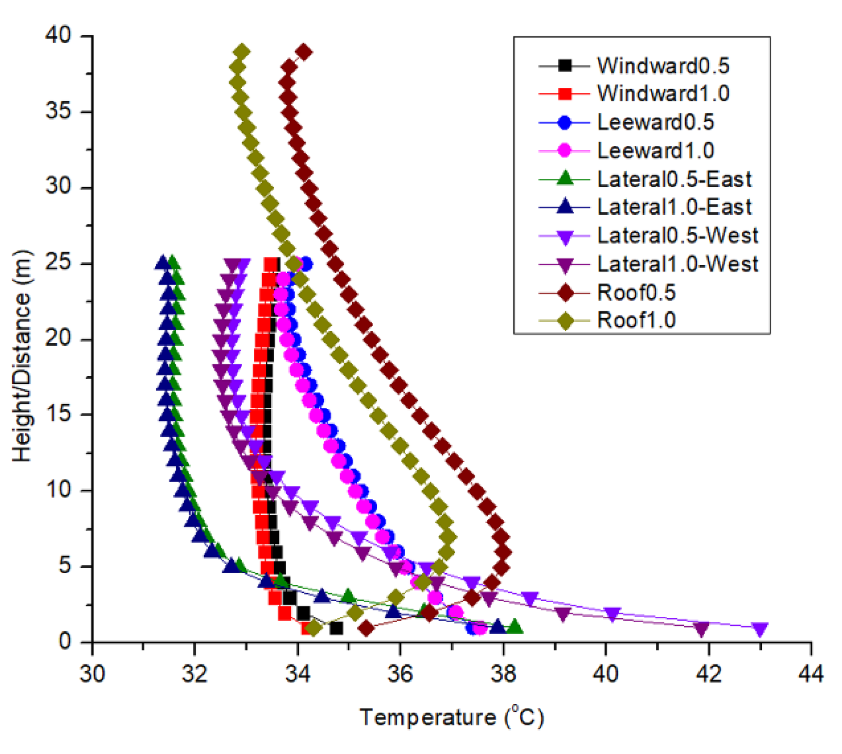
Temperature profiles at 0.5 and 1.0 m away from windward, leeward, lateral, and roof surfaces are separately provided in Figure 10. The temperature variation trend between 0.5 and 1.0 m away from the building surface presented better agreement. The temperature differences adjacent to windward, leeward, and lateral east surfaces showed negligible variations. While for the lateral west surface, due to the effect of solar radiation, the discrepancy is slightly larger than the above ones. The maximum temperature difference is approximately 1.0 °C adjacent to the ground. Because the solar heat flux significantly affected the thermal environment near the building rooftop, the temperature difference occurred at the locations of 0.5 and 1.0 m away from the roof surface. The maximum difference was around 1.5 °C located upstream and downstream of the rooftop, with larger turbulence, as remarkably shown in Figure 11.
Figure 11 shows the vertical distribution of the air temperature and airflow vector in the urban neighborhood. The air flow was characterized by skimming across the tops of building of interest and surrounding buildings due to the slightly denser terrain zone type. This phenomenon was mostly attributed to the fact that the incoming wind was perpendicular with the windward surface of Susquehanna North and the front two buildings. Meanwhile, the temperature distribution inside the street canyon presented the distinguishing change compared to the zone far from the buildings. Additionally, there was larger vortex created behind the building of interest, resulting in a slightly lower temperature distribution in contrast with upstream vortexes. Specifically, the temperature adjacent to the rooftop of the building of interest was remarkably larger than same height locations, taking in account the stronger impingement to windward and the weak flow across the roof.
This study also extracted centerline air temperatures at 0.5 and 1.0 m away from the building wall from the CFD simulations to analyze the velocity variation. Figure 12 shows the velocity magnitude profiles at 0.5 and 1.0 m away from windward, leeward, lateral, and roof surfaces. First, the lateral velocity profiles were consistent with the inlet boundary profile, although the flow almost attached to the lateral surfaces. The windward velocity profiles showed a slight increase due to the impingement and recirculation around the building, especially the leeward velocity profile, which had less variation. While, the velocity magnitudes at 0.5 and 1.0 m away from the rooftop ranged from 0.1 to 3.3 m/s, which were mainly affected by reattachment adjacent to the surface, especially at the upstream locations.
For the profiles between 0.5 and 1.0 m/s, the significant discrepancies about 0.5 m/s among those velocity profiles occured at the upstream locations adjacent to the building rooftop, and about 0.3 m/s at the zone between 5 to 25 m height adjacent to the lateral east surface. The front one was mainly induced by the flow characteristic of the skimming regime, as described above. The latter one arised from the narrow distance to the surrounding building, which significantly changed the flow field, while both lateral sides had the similar velocity variation trend. The velocity varied less (about 0.05 m/s) at the leeward surface because of the weak circulation between the downstream buildings. In summary, the pictures in this section presented the local velocity and temperature distribution and variations, which indicated the local microclimate characteristics of the decrease of wind speed and the increase of temperature around the building of interest in the urban neighborhood. Therefore, this section compared and quantified the impact of the local thermal environment on the building energy consumption due to the changes of local parameters, such as CHTCs, COP, and infiltration.
3.2. The Effect of CHTC on Energy Consumption
To investigate the CHTC characteristic in the urban neighborhood, Figure 13 first shows the distribution of the CHTC on the building and ground surfaces. The maximum CHTC values can reach up to 15.0 W/(m2·K). It was found that the CHTC in the windward surface and upstream locations of roof and lateral surfaces present significantly larger values compared to other locations in this building, as well as surrounding buildings. This pattern of CHTC distribution was mainly due to the slightly unobvious bounded vortex and horseshoe vortex around the building of interest, compared to that which appeared in the isolated building. A relatively well-defined logarithmic wind velocity profile resulted in larger and larger CHTC distribution, from the bottom to the top, in the windward surface, where relatively sufficient spacing around the surrounding buildings occurs. In addition, the small and weak vortex circulations, behind the building and downstream of the lateral surface, led to inferior CHTC distribution.
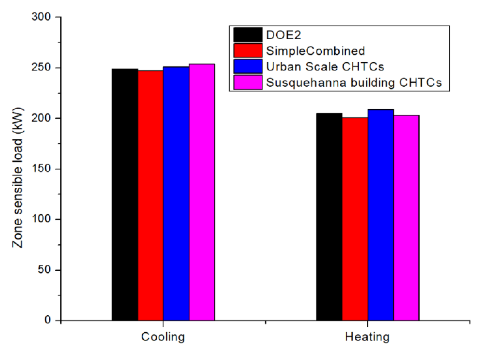
This study employed four different CHTC correlations, including the default CHTC equation in the EnergyPlus program, DOE-2, SimpleCombined correlations, urban-scale CHTC correlations [13], and newly derived from the above CFD simulation of Susquehanna North. Figure 14 shows zone-sensible cooling and heating loads with different CHTC correlations. The discrepancy among those cases showed slight influence of CHTC on maximum sensible load, in which the maximum variations existed; 1.95% for sensible cooling load and 3.82% for sensible heating load. Figure 15 shows the annual cooling and heating energy used with different CHTC correlations. It was found that the discrepancy still shows an undistinguishing impact of CHTC on the building energy use, in which the maximum variations were 1.21% and 0.89% for annual cooling energy use and annual heating energy use, respectively. Note that due to variant heating schedules defined in the energy model, the changes of heating consumption were not coinciding with cooling energy consumption.
Although only a slight effect from different CHTC correlations on energy consumption appears, it has to be admitted that Susquehanna North can consume up to 600 GJ for cooling energy use and 1120 GJ for heating energy use. The important aim of this model was to assess the impacts of outdoor air on building cooling systems. The model had 52 thermal zones designed in EnergyPlus, of which four of them are core zones and the rest of them are a combination of core–perimeter zones. It is important to note that 49 thermal zones are specifically simulated and are affected by the exterior-surface CHTC distribution. In summary, this present study provided a relatively accurate qualification of CHTC correlations on sensible load and building energy use, in comparison with an ideal air load system with a regular building layout [13].
3.3. The Effect of Local Air Temperature on COP
This study employed CFD simulation to predict the flow field around the urban neighborhood and exports the local air temperature to calculate the COP of the HVAC system due to the effect of the local microclimate environment. Figure 16 illustrates the COP profiles at the vertical/horizontal centerline 0.5 m away from different windward, leeward, lateral, and roof surfaces using three COP equations, as shown in Equations (12)–(14). Among the specific equations, the majority of COP values ranged from 2.0 to 2.7, except for Equation (13) that presented larger variations at the centerline 0.5 m away from the roof and leeward surfaces. This was mainly induced by the higher air temperature distribution affected by weak vortex circulations downstream of the building of interest, and direct solar radiation on the rooftop at noon. Moreover, the minimum value of about 0.25 was obtained by using Equation (13) near the lateral-west surface. This presented the larger variations of COP values. This phenomenon was bound with the larger temperature profiles as it was shown in Figure 10, in which the temperature profiles adjacent to west surfaces illustrated the larger variation pattern. Overall, the COP values in the lateral sides of the building of interest showed a significant variation, with both the increase of COP and height, and the decrease of temperature.
In order to capture the effect of local urban neighborhood characteristics on COP, the spatial surface-based COP distributions were calculated. Figure 17 shows the surface COP box charts 0.5 m away from different windward, leeward, lateral, and roof surfaces. For each surface, COP values were calculated every 1.0 m in two directions. For examples, there are 28 × 26 simulated points exported for analysis on the windward surface. It was found that the majority of averaged COP values calculated using Equations (12) and (14) were in the region of 2.1 to 2.6 at the simulation time of 12:00. The maximum COP value in all surfaces can reach up to 2.7, which are located in the lateral-east surface and upstream of the roof surface, due to less solar radiation influence and larger separation on the roof. Correspondingly, COP values at the rooftop had slightly larger variations, and COP values near the lateral east surface had slightly smaller variations compared to other surfaces among those three equations. In addition, COP values calculated by Equation (13) present a broader range and extremely lower values due to high air temperature adjacent to the lateral-west surface. However, it should be noted that more than 90% of COP values in this surface are acceptable and larger than 1.25. Overall, the COP values in the lateral-west side and roof side of the building of interest showed larger variation in the simulation period.
3.4. The Effect of Air Infiltration on Energy Consumption
This study extracted four different horizontal lines of air temperature, including 0.5, 1, 5, and 10 m away from the windward surface of the building of interests, to determine the local wind velocities. Table 5 illustrates the local averaged wind velocities located in the front of the building and 10 m above the ground. It was found that, compared to the incoming wind velocity with U = 5.0 m/s at the height of 10 m, the local wind velocities decreased significantly. The minimum local velocity factor 5.0 m away from the building wall was decreased to 0.294, indicating less than one-third incoming velocity magnitude against the windward surface. While, other local velocity factors showed less variations for 0.5, 1, and 10 m. Therefore, it was important to note that this study used the average horizontal line of the CFD-simulated distribution to generate the local velocity factor and to write into the new EPW weather data file. The results confirmed that it is important to consider wind sheltering effects by investigating the different urban terrain type.
Figure 18 shows the annual cooling and heating energy used with different infiltration calculation methods. A comparison indicated that the adjusted model had a significant impact on the energy consumption compared to other methods, with the maximum differences being up to 2.67% increase for cooling energy use and 2.18% decrease for heating energy use. Note that the adjusted model modified the default constant values of infiltration rate under all conditions in Equation (15) and Table 4. Therefore, the infiltration rate calculation method needs to be taken into account, especially for the urban neighborhood-based coefficients in the further study.
Besides the adjusted model, the other four methods considering the local velocity factor showed less discrepancies, with 1.93% change for annual cooling energy use and 1.14% for annual heating energy use. Although lower wind velocities around the building of interest resulted in small infiltration rates and slightly higher heat gain or heat loss, through the heat conduction of the building wall or window, the minor changes in the energy consumption for the building’s HVAC system were obtained due to limited thermal zones affected by infiltration closely related to the outdoor thermal environment. Therefore, it should be noted that the adjusted infiltration method is highly suitable for buildings with limited thermal zones or building energy consumption that is mainly dominated by the local micro-thermal environment.
4. Discussion
This study conducted a one-way coupling to model the urban microclimate environment and its effect on building energy use in a real academic building in University Park, USA. The steady-state calculation considering the solar irradiance was used to get the relatively accurate results of the local parameters. Although there are some limitations, for example, the fixed boundary conditions at specific date and time instead of transient cases, the local parameters in the microclimate environment were utilized to generate the correlations of CHTCs, which is not a specific value. Compared with the two-way coupling strategy, as previously shown in other studies [27,32,42,43], the steady-state calculation and the one-way coupling method from CFD to BES is acceptable as long as the relatively accurate CFD calculation is used. However, for the purpose of this study, employing the one-way coupling method was sufficient due to the limitation of computational resources, especially for a case study. However, further studies need take into account more comprehensive and actual descriptions and simulations, especially in the time period of one day or one week.
Moreover, this study made many simple assumptions, such as the uniform surface emissivity, regular building shapes, as well as neglecting the transpiration cooling effect by trees and grass. Those assumptions resulted in some uncertainties in the cooling/heating energy use due to the inaccurate local parameters from the CFD simulation. However, we have to acknowledge that it is a complex process to consider all aspects and conduct transient simulations for such a large simulation domain, in other words, those assumptions were chosen mostly due to the current computational ability for a large simulation domain with extensive buildings. Moreover, the verification and validation process should be dedicatedly considered, for example, the CFD simulation setup, the grid independence analysis, and the building energy model setup. Therefore, further studies need to seriously control the quality of results from the CFD and BES.
5. Broader Implications
While currently more than half of the population lives in urban areas, more than 80% of the population in some developed countries reside in urban areas. Major cities such as Los Angles and New York City in the US, or Shanghai in China, could benefit from the results of this study to design more sustainable and energy efficient urban neighborhoods. The results of this study lay out a framework on how to consider the influence of the outdoor air thermo-fluid emerging properties to assess and predict building energy consumption patterns. Therefore, future design of urban neighborhoods in major cities should benefit from outdoor airflow simulations coupled with building energy simulations in order to predict energy consumption of buildings.
This study considered the influence of the urban neighborhood on the efficiency of the cooling system with the use of the simulated outdoor air temperature. A more practical approach could benefit from the influence of the HVAC systems on the distribution of the outdoor air temperature and velocity as well. HVAC systems reject anthropogenic heat transfer, including sensible and latent heat transfer, to the outdoor air [47]. Heat rejection from the HVAC systems also could have influence on the outdoor air temperature and velocity around buildings. The rate of the latent and sensible heat transfer depends on the HVAC cooling system. Therefore, the accurate analysis of anthropogenic heat rejected from HVAC is necessary to evaluate the influence of the urban microclimate in further studies.
Another approach to include the influence of the urban microclimate on building energy consumption patterns could be to consider transient coupling on the CFD and building energy simulations [48]. Due to the complex nature of transient coupling simulations, a large number of studies consider steady-state conditions to predict various aspects of the local thermal environments [49,50,51,52]. A practical approach to reduce the complexity of the simulations could benefit from daily coupling, rather than finer granularity coupling, as coupling at each time step or at each hour is very costly. Granular coupling is only applicable for a short period of time. Even with any potential transient coupling, the outcomes of the coupled simulations may not enhance the accuracy of the coupled simulations significantly [48]. For example, daily coupling provides improvement for only up to 2.5% using the airport weather data and simulated data. Configuration of the urban neighborhood could enforce the coupling strategy. Potential influential variables are urban plan area density, size of the buildings, height variation of the buildings, and land coverage.
Another implication of this study is to address the built environment challenges, such as higher outdoor air temperature, energy demand, and greenhouse gas emissions, while sustaining a healthy environment. The solution requires the consideration and identification of different aspects in order to solve the problems associated with them. This enables advancing the understanding of energy and airflows in the built environment.
Current building energy simulation tools (e.g., EnergyPlus) accept average velocity values for the windward and leeward surfaces. The results of the CFD simulations conducted in this study showed spatial fluctuations in the velocity, at least for the windward side. With the improvement of the building energy simulation tools, there might be opportunities to assess the impact of spatial velocity fluctuations on the simulated results.
6. Conclusions
The present study conducted a parametric study to assess the impacts of the urban microclimate on thermo-fluid properties, including temperature and velocity, that led to different estimations of convective heat transfer rate, efficiency of building cooling systems, and infiltration rate of the buildings located in the built environment. The aim of this study was to quantitatively evaluate the influence of each parameter, CHTCs, infiltration rate, and COP on building energy use. Consequently, this study encompassed a one-way coupling simulation of CFD and BES to calculate the local temperature and velocity first in CFD simulations, with the heat flux boundary conditions from Radiance simulation. To evaluate impacts of convective heat transfer, two approaches were used to calculate outdoor CHTCs: (i) Use of previously-developed urban-scale CHTCs that required implementation of local air temperature and speed; and (ii) performing CFD simulations for an actual urban neighborhood and calculating detailed CHTCs on the ground and building surfaces. The discrepancy among those cases showed slight influence of CHTC on sensible load, in which the maximum variations existed; 1.95% for sensible cooling load and 3.82% for sensible heating load. Additionally, the discrepancy still showed an undistinguishing impact of CHTC on the building energy uses, in which the maximum variations were 1.21% and 0.89% for annual cooling energy use and annual heating energy use, respectively.
Implementation of CHTCs only had minor influence on the annual heating and cooling, which indicated, for recently retrofitted buildings, outdoor convection was not a significant major contributor to annual heating and cooling. In addition, it is important to note that, currently, BES, such as EnergyPlus, cannot accept detailed CHTCs. Therefore, the only option to implement CHTCs in EnergyPlus is to rely on averaged values for the roof, leeward, windward, and lateral walls.
The second contributor to the building energy consumption, especially cooling consumption, was the efficiency of the cooling systems. Three equations were selected to quantify the impacts of the urban microclimate on the COP of cooling systems. The results showed that the optimal locations for the installation of the cooling systems are on the windward wall and upstream roof. Installation of cooling systems on the leeward walls of buildings located in the built environment may lead to lower operational COP than the design COP. This was due to the fact that, with the higher temperature, there was less opportunity for the cooling system to exchange heat with outside.
The final variable was the consideration of the infiltration rate in the building energy consumption using recently-developed infiltration rate coefficients. The design flow rate method in EnergyPlus can take into the account the local velocity and temperature as long as the coefficients in the calculation are not zero. The results of this study showed, for buildings located in a fairly dense urban neighborhood, the adjusted infiltration model played a more important role in influencing the annual heating and cooling consumption than the default infiltration model.
Author Contributions
Conceptualization, J.L. and M.H.; funding acquisition, J.L. and J.S.; methodology, J.L., M.H. and S.K.N.; supervision, J.S.; writing—original draft, J.L. and M.H.; writing—review and editing, J.L., M.H., N.W.M. and J.S.
Funding
This study was sponsored by the National Natural Science Foundation of China (NSFC, No. 51608310) and the Science and Technology Plan Project of University in Shandong Province (J16LG07). The APC was funded by NSFC (No. 51608310).
Acknowledgments
This study is also supported by the Cluster of Sustainability at the University of Maryland (CITY@UMD). The Shandong Province Green Building Collaborative Innovation Center Innovation Team Support Program is specially acknowledged.
Conflicts of Interest
The authors declare that they have no conflicts of interest to this work.
References
- Makvandi, M.; Li, B.; Elsadek, M.; Khodabakhshi, Z.; Ahmadi, M. The Interactive Impact of Building Diversity on the Thermal Balance and Micro-Climate Change under the Influence of Rapid Urbanization. Sustainability 2019, 11, 1662. [Google Scholar] [CrossRef]
- Yiannakou, A.; Salata, K.-D. Adaptation to Climate Change through Spatial Planning in Compact Urban Areas: A Case Study in the City of Thessaloniki. Sustainability 2017, 9, 271. [Google Scholar] [CrossRef]
- Deng, Y.; Feng, Z.; Fang, J.; Cao, S.-J. Impact of ventilation rates on indoor thermal comfort and energy efficiency of ground-source heat pump system. Sustain. Cities Soc. 2018, 37, 154–163. [Google Scholar] [CrossRef]
- Kim, M.K.; Liu, J.; Cao, S.-J. Energy analysis of a hybrid radiant cooling system under hot and humid climates: A case study at Shanghai in China. Build. Environ. 2018, 137, 208–214. [Google Scholar] [CrossRef]
- Kong, X.-R.; Deng, Y.; Li, L.; Gong, W.-S.; Cao, S.-J. Experimental and numerical study on the thermal performance of ground source heat pump with a set of designed buried pipes. Appl. Therm. Eng. 2017, 114, 110–117. [Google Scholar] [CrossRef]
- Liu, J.; Xie, X.; Qin, F.; Song, S.; Lv, D. A case study of ground source direct cooling system integrated with water storage tank system. Build. Simul. 2016, 9, 659–668. [Google Scholar] [CrossRef]
- Liu, J.; Zhu, S.; Kim, M.K.; Srebric, J. A Review of CFD Analysis Methods for Personalized Ventilation (PV) in Indoor Built Environments. Sustainability 2019, 11, 4166. [Google Scholar] [CrossRef]
- Udara Willhelm Abeydeera, L.H.; Wadu Mesthrige, J.; Samarasinghalage, T.I. Global Research on Carbon Emissions: A Scientometric Review. Sustainability 2019, 11, 3972. [Google Scholar] [CrossRef]
- Choi, Y.; Lee, S.; Moon, H. Urban Physical Environments and the Duration of High Air Temperature: Focusing on Solar Radiation Trapping Effects. Sustainability 2018, 10, 4837. [Google Scholar] [CrossRef]
- Santillán-Soto, N.; García-Cueto, O.R.; Lambert-Arista, A.A.; Ojeda-Benítez, S.; Cruz-Sotelo, S.E. Comparative Analysis of Two Urban Microclimates: Energy Consumption and Greenhouse Gas Emissions. Sustainability 2019, 11, 2045. [Google Scholar] [CrossRef]
- Lundgren, K.; Kjellstrom, T. Sustainability Challenges from Climate Change and Air Conditioning Use in Urban Areas. Sustainability 2013, 5, 3116–3128. [Google Scholar] [CrossRef] [Green Version]
- Allegrini, J.; Dorer, V.; Carmeliet, J. Coupled CFD, radiation and building energy model for studying heat fluxes in an urban environment with generic building configurations. Sustain. Cities Soc. 2015, 19, 385–394. [Google Scholar] [CrossRef]
- Liu, J.; Heidarinejad, M.; Gracik, S.; Srebric, J. The impact of exterior surface convective heat transfer coefficients on the building energy consumption in urban neighborhoods with different plan area densities. Energy Build. 2015, 86, 449–463. [Google Scholar] [CrossRef]
- Yang, X.; Zhao, L.; Bruse, M.; Meng, Q. An integrated simulation method for building energy performance assessment in urban environments. Energy Build. 2012, 54, 243–251. [Google Scholar] [CrossRef]
- Toparlar, Y.; Blocken, B.; Maiheu, B.; van Heijst, G.J.F. A review on the CFD analysis of urban microclimate. Renew. Sustain. Energy Rev. 2017, 80, 1613–1640. [Google Scholar] [CrossRef]
- Montazeri, H.; Blocken, B.; Derome, D.; Carmeliet, J.; Hensen, J.L.M. CFD analysis of forced convective heat transfer coefficients at windward building facades: Influence of building geometry. J. Wind Eng. Ind. Aerodyn. 2015, 146, 102–116. [Google Scholar] [CrossRef] [Green Version]
- Vollaro, A.D.L.; Galli, G.; Vallati, A. CFD Analysis of Convective Heat Transfer Coefficient on External Surfaces of Buildings. Sustainability 2015, 7, 9088–9099. [Google Scholar] [CrossRef] [Green Version]
- Liu, J.; Heidarinejad, M.; Gracik, S.; Srebric, J.; Yu, N. An indirect validation of convective heat transfer coefficients (CHTCs) for external building surfaces in an actual urban environment. Build. Simul. 2015, 8, 337–352. [Google Scholar] [CrossRef]
- Emmel, M.G.; Abadie, M.O.; Mendes, N. New external convective heat transfer coefficient correlations for isolated low-rise buildings. Energy Build. 2007, 39, 335–342. [Google Scholar] [CrossRef]
- Botham-Myint, D.; Recktenwald, G.W.; Sailor, D.J. Thermal footprint effect of rooftop urban cooling strategies. Urban Clim. 2015, 14, 268–277. [Google Scholar] [CrossRef] [Green Version]
- Blocken, B.; Defraeye, T.; Derome, D.; Carmeliet, J. High-resolution CFD simulations for forced convective heat transfer coefficients at the facade of a low-rise building. Build. Environ. 2009, 44, 2396–2412. [Google Scholar] [CrossRef]
- Allegrini, J.; Dorer, V.; Carmeliet, J. Analysis of convective heat transfer at building façades in street canyons and its influence on the predictions of space cooling demand in buildings. J. Wind Eng. Ind. Aerodyn. 2012, 104–106, 464–473. [Google Scholar] [CrossRef]
- Liu, J.; Srebric, J.; Yu, N. Numerical simulation of convective heat transfer coefficients at the external surfaces of building arrays immersed in a turbulent boundary layer. Int. J. Heat Mass Transf. 2013, 61, 209–225. [Google Scholar] [CrossRef]
- Huang, J.; Gurney, K.R. The variation of climate change impact on building energy consumption to building type and spatiotemporal scale. Energy 2016, 111, 137–153. [Google Scholar] [CrossRef] [Green Version]
- De Lieto Vollaro, A.; De Simone, G.; Romagnoli, R.; Vallati, A.; Botillo, S. Numerical Study of Urban Canyon Microclimate Related to Geometrical Parameters. Sustainability 2014, 6, 7894–7905. [Google Scholar] [CrossRef] [Green Version]
- Sun, Y.; Heo, Y.; Tan, M.; Xie, H.; Jeff Wu, C.F.; Augenbroe, G. Uncertainty quantification of microclimate variables in building energy models. J. Build. Perf. Simul. 2014, 7, 17–32. [Google Scholar] [CrossRef]
- Heidarinejad, M.; Gracik, S.; Sadeghipour Roudsari, M.; Khoshdel Nikkho, S.; Liu, J.; Liu, K.; Pitchorov, G.; Srebric, J. Influence of building surface solar irradiance on environmental temperatures in urban neighborhoods. Sust. Cities Soc. 2016, 26, 186–202. [Google Scholar] [CrossRef] [Green Version]
- Sun, Y.; Su, H.; Wu, C.F.J.; Augenbroe, G. Quantification of model form uncertainty in the calculation of solar diffuse irradiation on inclined surfaces for building energy simulation. J. Build. Perf. Simul. 2014, 8, 253–265. [Google Scholar] [CrossRef]
- Liu, J.; Heidarinejad, M.; Pitchurov, G.; Zhang, L.; Srebric, J. An extensive comparison of modified zero-equation, standard k-ε, and LES models in predicting urban airflow. Sustain. Cities Soc. 2018, 40, 28–43. [Google Scholar] [CrossRef]
- Wong, N.H.; Jusuf, S.K.; Syafii, N.I.; Chen, Y.X.; Hajadi, N.; Sathyanarayanan, H.; Manickavasagam, Y.V. Evaluation of the impact of the surrounding urban morphology on building energy consumption. Solar Energy 2011, 85, 57–71. [Google Scholar] [CrossRef]
- Li, J.; Liu, J.; Srebric, J.; Hu, Y.; Liu, M.; Su, L.; Wang, S. The Effect of Tree-Planting Patterns on the Microclimate within a Courtyard. Sustainability 2019, 11, 1665. [Google Scholar] [CrossRef]
- Srebric, J.; Heidarinejad, M.; Liu, J. Building neighborhood emerging properties and their impacts on multi-scale modeling of building energy and airflows. Build. Environ. 2015, 91, 246–262. [Google Scholar] [CrossRef]
- Dols, W.S.; Emmerich, S.J.; Polidoro, B.J. Using coupled energy, airflow and indoor air quality software (TRNSYS/CONTAM) to evaluate building ventilation strategies. Build. Serv. Eng. Res. Technol. 2015, 37, 163–175. [Google Scholar] [CrossRef] [PubMed] [Green Version]
- Miller, C.; Thomas, D.; Kämpf, J.; Schlueter, A. Urban and building multiscale co-simulation: Case study implementations on two university campuses. J. Build. Perf. Simul. 2018, 11, 309–321. [Google Scholar] [CrossRef]
- Zuo, W.; Wetter, M.; Tian, W.; Li, D.; Jin, M.; Chen, Q. Coupling indoor airflow, HVAC, control and building envelope heat transfer in the Modelica Buildings library. J. Build. Perf. Simul. 2016, 9, 366–381. [Google Scholar] [CrossRef]
- Greenshields, C.J. OpenFOAM user guide. In OpenFOAM Foundation Ltd, version 6; 2018; Available online: https://cfd.direct/openfoam/user-guide/ (accessed on 5 September 2019).
- Hargreaves, D.M.; Wright, N.G. On the use of the k– model in commercial CFD software to model the neutral atmospheric boundary layer. J. Wind Eng. Ind. Aerodyn. 2007, 95, 355–369. [Google Scholar] [CrossRef]
- Blocken, B.; Stathopoulos, T.; Carmeliet, J. CFD simulation of the atmospheric boundary layer: wall function problems. Atmos. Environ. 2007, 41, 238–252. [Google Scholar] [CrossRef]
- Roache, P.J. Quantification of uncertainty in computational fluid dynamics. Ann. Rev. Fluid Mech. 1997, 29, 123–160. [Google Scholar] [CrossRef]
- Energyplus. EnergyPlus Engineering Reference; Ernest Orlando Lawrence Berkeley National Laboratory: Berkeley, CA, USA, 2017. [Google Scholar]
- Deru, M.; Field, K.; Studer, D.; Benne, K.; Griffith, B.; Torcellini, P.; Liu, B.; Halverson, M.; Winiarski, D.; Yazdanian, M.; et al. U.S. Department of Energy Commercial Reference Building Models of the National Building Stock; NREL/TP-5500-46861; NREL: Golden, CO, USA, 2011. [Google Scholar]
- Khoshdel Nikkho, S.; Heidarinejad, M.; Liu, J.; Srebric, J. Quantifying the impact of urban wind sheltering on the building energy consumption. Appl. Therm. Eng. 2017, 116, 850–865. [Google Scholar] [CrossRef] [Green Version]
- Gracik, S.; Heidarinejad, M.; Liu, J.; Srebric, J. Effect of urban neighborhoods on the performance of building cooling systems. Build. Environ. 2015, 90, 15–29. [Google Scholar] [CrossRef]
- Chow, T.T.; Lin, Z.; Yang, X.Y. Placement of condensing units of split-type air-conditioners at low-rise residences. Appl. Therm. Eng. 2002, 22, 1431–1444. [Google Scholar] [CrossRef]
- Variable Rate Rooftop Unit Test (VRTUT) Report; Northwest Energy Efficiency Alliance (NEEA): Vancouver, WA, Canada, 2013; Available online: https://neea.org/docs/default-source/reports/variable-rate-rooftop-unit-test.pdf?sfvrsn=5 (accessed on 5 September 2019).
- Ng, L.C.; Persily, A.K.; Emmerich, S.J. Improving infiltration modeling in commercial building energy models. Energy Build. 2015, 88, 316–323. [Google Scholar] [CrossRef]
- González, J.E.; Gutierrez, E. In On the Environmental Sensible/Latent Heat Fluxes From A/C Systems in Urban Dense Environments: A New Modeling Approach and Case Study, ASME. In Proceedings of the Symposium on Integrated/Sustainable Building Equipment and Systems, San Diego, CA, USA, 28 June–2 July 2015. [Google Scholar]
- Liu, J.; Heidarinejad, M.; Guo, M.; Srebric, J. Numerical Evaluation of the Local Weather Data Impacts on Cooling Energy Use of Buildings in an Urban Area. Procedia Eng. 2015, 121, 381–388. [Google Scholar] [CrossRef] [Green Version]
- Alexandri, E.; Jones, P. Temperature decreases in an urban canyon due to green walls and green roofs in diverse climates. Build. Environ. 2008, 43, 480–493. [Google Scholar] [CrossRef]
- Chen, H.; Ooka, R.; Huang, H.; Tsuchiya, T. Study on mitigation measures for outdoor thermal environment on present urban blocks in Tokyo using coupled simulation. Build. Environ. 2009, 44, 2290–2299. [Google Scholar] [CrossRef]
- Hang, J.; Luo, Z.; Sandberg, M.; Gong, J. Natural ventilation assessment in typical open and semi-open urban environments under various wind directions. Build. Environ. 2013, 70, 318–333. [Google Scholar] [CrossRef]
- Santamouris, M. On the energy impact of urban heat island and global warming on buildings. Energy Build. 2014, 82, 100–113. [Google Scholar] [CrossRef]
Figure 1.
Aerial of the selected neighborhood with the building of interest (Susquehanna North) identified in the red box (latitude: 38°98′55.4″ N, longitude: 76°56′37.7″ W, scale: 1:5000).
Figure 1.
Aerial of the selected neighborhood with the building of interest (Susquehanna North) identified in the red box (latitude: 38°98′55.4″ N, longitude: 76°56′37.7″ W, scale: 1:5000).

Figure 2.
Simplified simulation framework for the co-simulation of computational fluid dynamics (CFD) and building energy simulation (BES) (EPW—EnergyPlus weather data (EPW), met—weather station meteorological data, loc—local meteorological data around the building of interest).
Figure 2.
Simplified simulation framework for the co-simulation of computational fluid dynamics (CFD) and building energy simulation (BES) (EPW—EnergyPlus weather data (EPW), met—weather station meteorological data, loc—local meteorological data around the building of interest).

Figure 3.
CFD mesh distribution: (a) The block mesh in the simulated domain, (b) the mesh adjacent to the building of interest, and (c) the boundary layer close to building wall.
Figure 3.
CFD mesh distribution: (a) The block mesh in the simulated domain, (b) the mesh adjacent to the building of interest, and (c) the boundary layer close to building wall.

Figure 4.
y+ profiles at the centerline locations in the windward, leeward, lateral, and roof surfaces.
Figure 4.
y+ profiles at the centerline locations in the windward, leeward, lateral, and roof surfaces.

Figure 5.
Distribution of average and max y+ for the corresponding patches in the building of interest.
Figure 5.
Distribution of average and max y+ for the corresponding patches in the building of interest.

Figure 6.
The imposed heat fluxes (w/m2) on the building and ground surfaces.

Figure 7.
EnergyPlus/OpenStudio models for the case study building.

Figure 8.
CHTCs profiles along the centerline locations in the windward, leeward, lateral, and roof surfaces.
Figure 8.
CHTCs profiles along the centerline locations in the windward, leeward, lateral, and roof surfaces.

Figure 9.
Distribution of the temperature (K) around the building of interest in the urban neighborhood.
Figure 9.
Distribution of the temperature (K) around the building of interest in the urban neighborhood.

Figure 10.
Temperature profiles at 0.5 and 1.0 m away from windward, leeward, lateral, and roof surfaces.
Figure 10.
Temperature profiles at 0.5 and 1.0 m away from windward, leeward, lateral, and roof surfaces.

Figure 11.
Distribution of the air temperature and airflow vector in the urban neighborhood.

Figure 12.
Velocity magnitude profiles at 0.5 and 1.0 m away from windward, leeward, lateral, and roof surfaces.
Figure 12.
Velocity magnitude profiles at 0.5 and 1.0 m away from windward, leeward, lateral, and roof surfaces.

Figure 13.
Distribution of the CHTC on the building of interest and surrounding buildings.

Figure 14.
The maximum zone sensible cooling and heating loads with different CHTC correlations.

Figure 15.
The annual cooling and heating energy used with different CHTC correlations.

Figure 16.
COP profiles at the centerline 0.5 m away from different surfaces (C1, C2, and C3 represent three different COP equations shown in Equations (12)–(14), respectively).
Figure 16.
COP profiles at the centerline 0.5 m away from different surfaces (C1, C2, and C3 represent three different COP equations shown in Equations (12)–(14), respectively).

Figure 17.
COP box charts 0.5 m away from different surfaces (C1, C2, and C3 represent three different COP equations shown in Equations (12)–(14), respectively).
Figure 17.
COP box charts 0.5 m away from different surfaces (C1, C2, and C3 represent three different COP equations shown in Equations (12)–(14), respectively).

Figure 18.
The annual cooling and heating energy used with different infiltration calculation methods.
Figure 18.
The annual cooling and heating energy used with different infiltration calculation methods.


Table 1.
Summary of the energy model setup [42].
Table 1.
Summary of the energy model setup [42].
| Parameters | Summary |
|---|---|
| Information | Four floors, 3 m height each floor Weather: Actual methodological year (2014) at College Park, MD |
| Construction | Construction sets: the U.S. Department of Energy (DOE) Pre-1980 reference buildings |
| Spaces | Window to wall ratio: 33% Thermal zoning: Perimeter and core zoning with single space type Perimeter zone depth: 3 m |
| Loads | Lighting: 20 W/m2 Electric equipment: 10 W/m2 |
| Heating, Ventilation, and Air Conditioning (HVAC) | System: Rooftop variable air volume (VAV) with reheat Cooling: Direct expansion (DX) Heating: District heating Fan efficiency: 70% Ventilation: 0.3048 L/s·m2 (0.06 cfm/ft2) and 0.002360 m3/person (5 cfm/person) |
| Schedules | Operation at 07:00 to 16:00 |
| Setpoints | 24 °C (winter) to 26 °C (summer) |
Table 2.
ho,c correlations based on combined local velocities(Uloc) and the temperature difference (∆T) derived from the current CFD simulation.
Table 2.
ho,c correlations based on combined local velocities(Uloc) and the temperature difference (∆T) derived from the current CFD simulation.
| Surface | |
|---|---|
| Windward | (R = 0.91) |
| Leeward | (R = 0.87) |
| Roof | (R = 0.86) |
Table 3.
ho,c correlations’ combined Uloc and ∆T revised from urban-scale CHTC correlation [13].
Table 3.
ho,c correlations’ combined Uloc and ∆T revised from urban-scale CHTC correlation [13].
| Surface | |
|---|---|
| Windward | (R = 0.94) |
| Leeward | (R = 0.93) |
| Roof | (R = 0.91) |
Table 4.
Default and adjusted coefficients for the design rate model in the EnergyPlus Program.
| Coefficients | Default Value | Adjusted Value |
|---|---|---|
| A | 1 | 0 |
| B | 0 | 0.0318 |
| C | 0 | 0 |
| D | 0 | 0.0315 |
Table 5.
Local averaged wind velocities located in the front of building and 10 m above the ground.
| Distance from windward (m) | 0.5 | 1.0 | 5.0 | 10.0 |
| Averaged velocities (m/s) | 1.78 | 1.71 | 1.47 | 1.82 |
| Local velocity factor | 0.356 | 0.342 | 0.294 | 0.364 |
© 2019 by the authors. Licensee MDPI, Basel, Switzerland. This article is an open access article distributed under the terms and conditions of the Creative Commons Attribution (CC BY) license (http://creativecommons.org/licenses/by/4.0/).
Share and Cite
MDPI and ACS Style
Liu, J.; Heidarinejad, M.; Nikkho, S.K.; Mattise, N.W.; Srebric, J. Quantifying Impacts of Urban Microclimate on a Building Energy Consumption—A Case Study. Sustainability 2019, 11, 4921. https://doi.org/10.3390/su11184921
AMA Style
Liu J, Heidarinejad M, Nikkho SK, Mattise NW, Srebric J. Quantifying Impacts of Urban Microclimate on a Building Energy Consumption—A Case Study. Sustainability. 2019; 11(18):4921. https://doi.org/10.3390/su11184921
Chicago/Turabian StyleLiu, Jiying, Mohammad Heidarinejad, Saber Khoshdel Nikkho, Nicholas W. Mattise, and Jelena Srebric. 2019. "Quantifying Impacts of Urban Microclimate on a Building Energy Consumption—A Case Study" Sustainability 11, no. 18: 4921. https://doi.org/10.3390/su11184921
Note that from the first issue of 2016, this journal uses article numbers instead of page numbers. See further details here.