Identifying Spatial Patterns of Retail Stores in Road Network Structure


1
Key Laboratory of Geospatial Technology for the Middle and Lower Yellow River Regions (Henan University), Ministry of Education, Kaifeng 475004, China
2
College of Environment and Planning, Henan University, Kaifeng 475004, China
3
Institute of Henan Spatio-temporal Bigdata Industrial Technology, Henan University, Zhengzhou 450046, China
4
Urban Bigdata Institute, Henan University, Kaifeng 475004, China
5
Key Research Institute of Yellow River Civilization and Sustainable Development, Henan University, Kaifeng 475004, China
6
Department of Geography, University of Connecticut, Storrs, CT 06269, USA
*
Author to whom correspondence should be addressed.
Sustainability 2019, 11(17), 4539; https://doi.org/10.3390/su11174539
Submission received: 26 June 2019
/
Revised: 9 August 2019
/
Accepted: 16 August 2019
/
Published: 21 August 2019
(This article belongs to the Special Issue Sustainable Urban Planning Techniques)
Abstract
:Understanding the spatial patterns of retail stores in urban areas contributes to effective urban planning and business administration. A variety of methods have been proposed in the scientific literature to identify the spatial patterns of retail stores. These methods invariably employ arbitrary grid cells or administrative units (e.g., census tracts) as the fundamental analysis units. As most urban retail stores are distributed along street networks, using area-based analysis units is subject to statistical biases and may obfuscate the spatial pattern to some extent. Using the street segment as the analysis unit, this paper derives the spatial patterns of retail stores by crawling points of interest (POI) data in Zhengzhou, a city in central China. Then, the paper performs the network-based kernel density estimation (NKDE) and employs several network metrics, including the global, local, and weighted closeness centrality. Additionally, the paper discusses the correlation between the NKDE value and the closeness centrality across different store types. Further analysis indicates that stores with a high correlation tend to be distributed in city centers and subnetwork centers. The comparison between NKDE and cell-based KDE shows that our proposed method can address potential statistical issues induced by the area-based unit analysis. Our finding can help stakeholders better understand the spatial patterns and trends of small business expansion in urban areas and provide strategies for sustainable planning and development.
1. Introduction
Location is key to the success of the brick-and-mortar retail business. “Location, location, location,” as one of the oldest mantras in business planning and investment, has often been the primary business consideration when selecting an operating site. An excellent location may be enough to make a retailer successful even if its strategy is mediocre. Similarly, a poor location can be a significant burden that even a good retailer cannot overcome [1]. Finding the optimal location for a retail store and conducting retail location analyses have been longstanding aims of both retail business and urban planning. In the process of urban growth, the expansion of the city is increasingly dependent on the city’s function as a consumer hub [2,3]. The spatial configuration of the urban retail industry is of great significance for maximizing the economic benefits and optimizing the transport system [4]. Understanding the spatial distribution of commercial facilities is essential to the future planning of urban commercial retail systems and contribute to the efficient design of urban commercial space. Aiming at the sustainable development of the city, this improved understanding can avoid squandering planning resources that could be better allocated to other needs.
Traditional retail location analysis focuses on the trading-area and site selection of individual retail stores. These studies often use Reilly’s law or Huff’s model to infer the trading-area of stores or facilities [5,6] to determine the location of a restaurant in conjunction with the location-allocation model [7] in the context of Geographical Information Systems (GIS) [8]. Nevertheless, a single retail store “does not tell the whole story” [9]. From the perspective of spatial planning, the location of various types of retail stores determines the retail business structure of the city, which could be leveraged to uncover the market potential. Many cases have examined the spatial structure of retail commerce. Based on the central place theory, early studies defined the market area in a top-down hierarchical system, spatially forming a business center network that is triangular in shape and contains hexagonal market areas [10]. In addition, market, traffic, and public administration principles are used to shape diversified distribution systems [11]. Thus, the commercial spatial structure becomes a more diversified pattern when considering these non-spatial dimensions [12].
Given an increasing number of spatial analysis methodologies, most studies focused on the location of retail stores by applying GIS techniques. For example, Porto et al. studied commercial and service activities in Bologna, Italy. They discovered that retail and service activities in Bologna were generally concentrated in areas that enjoyed better centrality [13]. Similar conclusions were reached in a case study involving the correlation between retail stores and street networks in Barcelona [14], Spain and in Changchun [15], Guangzhou [16], and Wuhan, China [17]. By utilizing a grid cell as the analysis unit, the studies revealed the law of interaction between the location-distribution pattern of urban retail stores and the structure of street networks. However, there are noticeable statistical biases when using administrative units. First, the area-based unit analysis is subject to the classic modifiable areal unit problem (MAUP), referring to the effect that both the analysis scale (i.e., the smallest unit under observation) and the study scope considerably affect the statistical outcome. Second, using area-based units is subject to the “edge effect” introduced by the relative placement of urban retailers: In cities, the majority of stores are distributed along transport arterials, which are typically unit boundaries. Thus, comparing to random distributions, the spatial pattern of stores summarized by area-based units can be largely affected by the spatial organization of units [18]. To this end, it is better to characterize the spatial pattern of retail stores using network-based structure.
Traditionally, streets are part of the public transportation network, and thus, people pay more attention to their pass function. Since diverse urban economic activities occur on main streets, they involve not only traffic but also trading, peddling, and selling in a more general sense, as when Jacobs argued that streets are the lifeblood of cities rather than mere traffic channels [19,20,21,22]. As a public space that carries traffic, economic activities, and other events, streets connect urban functions physically and cognitively [22]. Early research on streets concentrated on road networks to explore an extension of the Huff model [23] or the space syntax analysis [24,25]. Itzhak et al. [26] applied the spatial syntax method to study the correlation between the spatial pattern of retail activities and the spatial configuration of road networks in eight Israeli cities. With the progress of network science, road network structures based on complex networks are receiving increasing levels of public attention. Wang et al. [27] took population census blocks as the analysis unit to quantitatively analyze the correlation between street centrality and land use intensity in Baton Rouge. In terms of land use types, Wang et al. [28] explored the relationship between street centrality and different types of urban land use in Shenzhen, China. Streets are also a key element in the urban image theory [29]. A series of cases have recently been conducted, including cases based on online street views [30,31,32,33,34]. By leveraging deep learning technology, Li et al. calculated the shadows of street trees in downtown Boston by determining the Sky View Factor (SVF) from street images [35]. They then analyzed the spatial distribution of solar radiation in the street canyons [36]. These studies reflect the unique value of the street as a line cell in urban research. To date, there are very few such studies employing the spatial structure of street networks for retail analysis.
In recent years, along with the rapid growth of mobile location-based service (LBS) technologies, a large amount of multi-source LBS data can be obtained from the public domain and social media. These data include points of interest (POIs), social network records, and cell phone signal. In addition to reflecting the human dynamics in cities, LBS data can be used to reveal the first-order distribution (e.g., economic indices, population intensity, condition of public facilities) and second-order characteristics (human movements, flow of goods, social ties) of urban properties to better understand the urban function, urban structure, and characteristics of crowd movement within a city [37,38]. For example, Wu et al. [39] studied and modeled crowd movement patterns of more than 15 million check-in records in Shanghai. Pucci et al. [40] analyzed urban residents’ spatiotemporal patterns and commuting characteristics in Milan, Italy, based on mobile signal data. There are rich semantic features for POI data, which could uncover the activity space in a city. Coupled with machine learning methods like topic modeling and word vector, employing POI data are able to identify urban functional areas with added semantic information [41,42] and classify urban land use with the support of remote sensing imagery [43,44].
Currently, POI data is widely used for urban studies, but the analysis unit is dominated by area-based grid cells. Streets and their near vicinity are the primary space for commercial activities to take place. Uncovering spatial patterns of retail stores in street unit can address potential statistical issues induced by the area-based unit analysis. Thus, studies employing street networks play an important role in the evaluation of the retail industry aimed at sustainable development [45,46]. In this paper, we take Zhengzhou, a city in central China, as an example to analyze the distribution patterns of different types of retail stores by using the street as the analysis unit. The paper also explores the correlation between the distribution of retail stores and the street centrality indicator. In terms of the spatial distribution pattern, we applied the network-based kernel density estimation to analyze the spatial distribution of six types of retail stores. After creating the road network data set, we calculated the global, local, and weight closeness centrality indicators separately. By focusing on a street as a linear analysis unit, this paper aims to reveal more detailed spatial distribution rules of different types of retail stores and to explore their interrelated characteristics with street closeness centrality. These multiple tiers of analyses can shed light on urban commercial facility planning and sustainable development.
The paper is organized as follows. Section 2 details the methodology of network-based kernel density estimation and the formation of closeness centrality. Section 3 describes our study area and data. Section 4 introduces the statistical and spatial distribution of different types of retail stores in a road network structure. Section 5 concludes the paper with implications for sustainable urban planning.
2. Methodology
2.1. Network-Based Kernel Density Estimation
The Kernel Density Estimation (KDE) method derives the density of the observations in terms of the continuous probability distribution of the point-based data [47]. The KDE estimates the density value at each location as the average value within a spatial window (i.e., the bandwidth) based on a kernel function. The kernel function is a continuous normalized function that is centered at a particular point and summarizes values within a given bandwidth [48], as defined by Equation (1).
where h is the bandwidth and x-xi indicates the distance between the center of the kernel (x) and the location xi. There are different types of kernels used for KDE. Here the popular quartic function is employed [15], as given by Equation (2).
where v is di/h (di is the distance from the kernel center), and T indicates the transpose of the matrix. Typically, the KDE uses grid cells as the analysis unit and the Euclidean distance as the distance metric. As the urban space is not homogenous because of the mixed land use and the structure of road networks, other forms of analysis units (e.g., census tracts) and distance metrics (e.g., the shortest path distance) have been applied to real-world density assessments.
The network-based kernel density estimation (NKDE) method is the network extension of the two-dimensional KDE. The distance metric employed by the NKED method is the shortest path distance, which avoids the oversimplified Euclidean distance measure. In addition, the topological relationship of the line elements in the network is considered. To avoid the overestimation of the density and improve the computational efficiency, the equal-split kernel function method is introduced to normalize the estimation results [49]. Suppose that the shortest path from x to xi contains p nodes: v1, …, vp and that ni represents the degree of the node vi, the form of the equal-split kernel function for the network-based kernel density estimator [50] is defined by Equation (3).
Stores may overlap in certain urban areas, such as near the central business district. To ensure the accuracy of the measure, overlapped store locations were treated as the same point. The point was weighted by the number of overlaps using the quantile mapping method, which could avoid the skewed distribution of stores in highly clustered areas [51]. Then the kernel density value was weighted for calculation. This method sorted the number of overlapped stores in ascending order, the the ranks were used to compute the normalized weight value. Given the store set as c, the weight is calculated by Equation (4).
where wk is the weight of the kth ranked store location (from the smallest to the largest), rmax and rmin are the user-defined parameters that control the influence of the weights on the kernel estimator, and they are set to 2 and 1, respectively; mc and me are the total count of the c and the number of equal values in c, respectively.
2.2. Closeness Centrality Index
The concept of closeness centrality has been used in the complex network theory [52,53]. It measures how central a node is with respect to other nodes in the network [54]. Urban roads are a typical spatial network which can be modeled by two methods. The first method is the primal network: The method defines the road intersection as nodes; then, the road segment with the real length is abstracted into the edge of the network. The other method is the dual network: The method abstracts the roads into nodes and the connection between road segments into edges of the network. Comparing to the dual network method, the primal network is able to retain the complete spatial network characteristics, such as position and distance, and is invariably adopted by most GIS [55]. For this reason, this paper employs the primal network and calculates the index of the closeness centrality () to measure the characteristics of the network nodes and edges. The closeness centrality is defined by Equation (5) [13].
where N is the total number of nodes in the network, and are the shortest path distance between nodes i and j.
The closeness centrality can be classified into the global closeness centrality (GCC) and the local closeness centrality (LCC). The former calculates all the nodes in the network, while the latter only involves nodes around a target node. To derive the LCC, an arbitrary distance value is usually applied to estimate the buffer of the node. For example, in the case of Barcelona, Porta et al. [14] defined three neighborhoods with a distance buffer of 800 m, 1600 m, and 2400 m, respectively. To overcome this arbitrary nature, a method based on the modularity indicator is used to define the buffer, generating network-based communities (or subnetworks). The modularity quantifies how good a community or a network partition is, as given by Equation (6) [56].
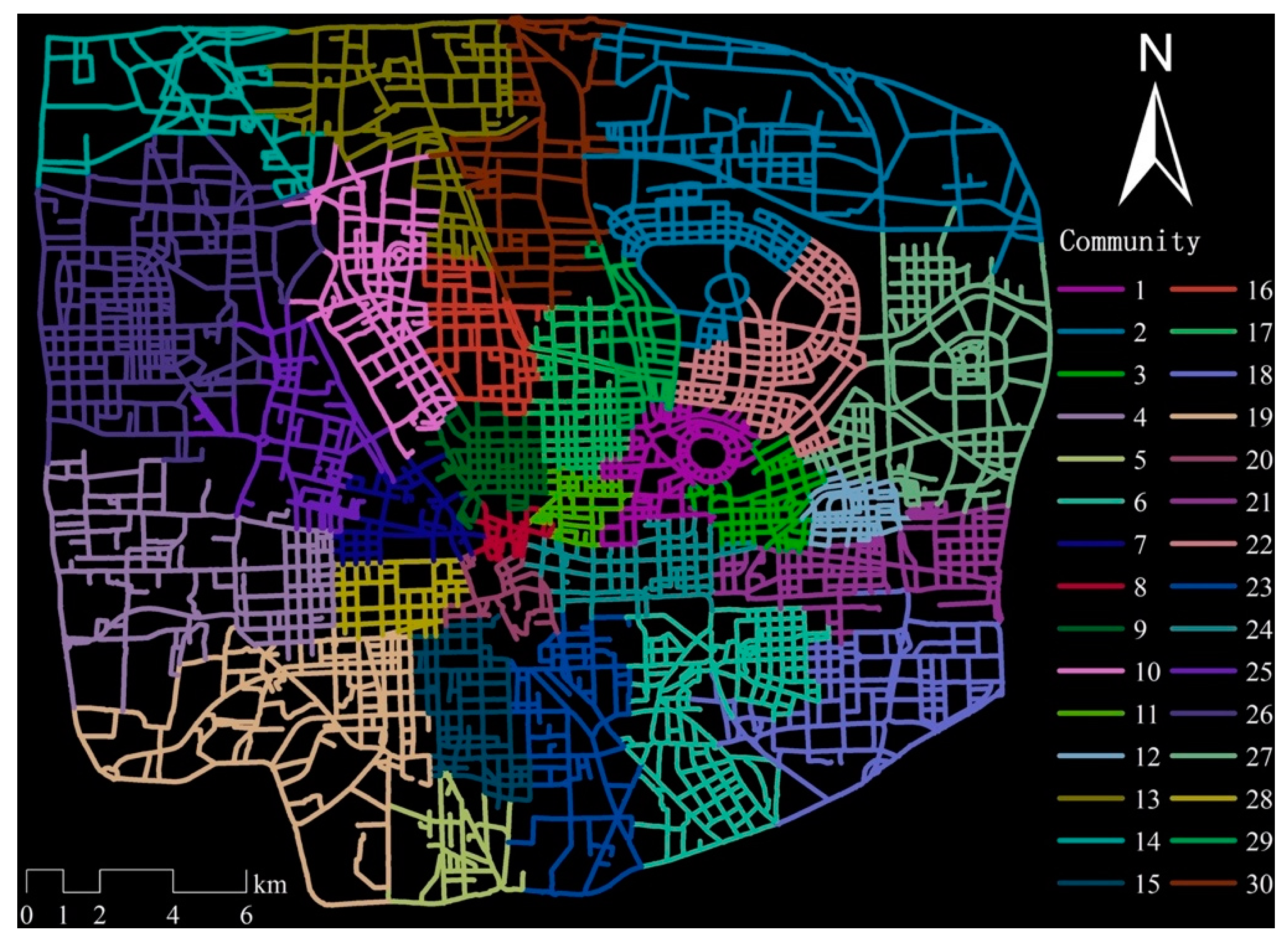
where is the number of subnetworks, is the number of edges within a subnetwork, is the total degree of nodes in the subnetwork, and is the total number of edges in the network. There are many modularity-based community detection algorithms (e.g., Fast unfolding, Combo, Informap, and Label propagation.) According to the study of Huang et al. [57], the Combo algorithm is more suitable for detecting spatial network communities. With the modularity value being the optimization objective, this algorithm discovers communities through three optimization strategies: Community division, community merging, and intercommunity node shift [58]. The weight of the edge is defined by the number of bus lines between nodes. The road network in the study area is thus divided into 30 subnetworks with a module value of 0.9046 by the Combo algorithm (Figure 1).
It can be seen that represents the global feature of the nodes in the network, while describes the local features. Because a road serves both the global (relative to the entire city) and the local (relative to the subnetwork) functions, the weighted value of the and is used as an aggregate measure of the closeness centrality of the node, as shown in Equation (7) [59].
where are the weight and the edge counts of the subnetwork m, respectively; is the inter edge counts between the subnetwork m and other subnetworks. The weighted closeness centrality of each node is calculated separately by Equation (7), and the average centrality value of the two nodes of the road segment is generated as the closeness centrality of the road segment. Here, the Urban Network Analysis tool developed by Sevtsuk et al. [60] was used to calculate the node closeness centrality.
3. Study Area and Data
Henan province is the most populous province in China, and its capital, Zhengzhou, is the political, economic, technical, and educational center of over 100 million people in central China. It is located on the south bank of the middle reaches of the Yellow River (Figure 1). It is found in China’s hinterland and is known colloquially as “the center of sky and earth.” The geographical coordinates of the city range from 112°42′–114°14′ E and 34°16′–34°58′ N. The total area of Zhengzhou is 7446 km2 with an urban area of 1010 km2 and a built-up area of 549.33 km2. The economy of Zhengzhou ranks third in central China and 17th among all Chinese cities in terms of GDP. In 2016, Zhengzhou was identified as one of the fastest-growing cities in China [61]. Moreover, Zhengzhou is located at the intersection of the national ordinary railway network and the high-speed railway network. The transportation advantages have made Zhengzhou a commercial and trade mecca in central China.
Our study area is the contiguously urbanized built-up area of Zhengzhou. The area is situated in central Zhengzhou, bounded on the north, east, west, and south of the 4th ring road of the city, as shown in Figure 1. This area was selected because of the large concentration of retail stores in the area. We extracted POI data using the application programming interface (API) from Baidu Maps (map.baidu.com) and Gaode Maps (www.amap.com), which are two primary mapping service providers in China, to construct a retail store dataset. Specifically, in order to obtain records for all retail stores, we generated regular grid rectangles as the querying region. The rectangle is 15” in width and 12” in height. There are 4133 rectangles in the study area. Each record collected contains a store’s name, address, and location coordinates.
We then divided the retail stores into six broad categories consisting of specialty stores (SS), department stores (DS), supermarkets (SMS), furniture stores (FS), construction material stores (CMS), and consumer product stores (CPS), which mirrors the classification system used by the Chinese government [12]. A specialty store is defined as a store that sells specific goods like clothes, footwear, electronic products, etc. It is further refined into seven subtypes such as office supply stores (OSS), apparel shop stores (AOS), home appliance stores (HAS), drug stores (DGS), car stores (CAS), cosmetic stores (CTS), and other stores (OTS). The spatial datasets of the retail stores and street network were built with ESRI ArcGIS. The final data set includes 78,777 retail stores (Table 1), 3523 network nodes, and 5569 network edges of the street with the red line in the study area, as illustrated in Figure 2.
4. Results and Discussion
4.1. Descriptive Statistics for Retail Stores
The results including the descriptive statistics of stores, roads, and line cells (with a length of 400 m where the stores are located) are given in Table 1. There are 41,769 SS distributed on 2285 roads and within 3335 line cells, with 18.28 stores on each road and 12.52 stores in each line cell on average. The second largest number comes from 16,900 CPS, which are evenly located in densely populated areas. The CMS, however, are concentrated in the urban fringe due to its demand for land use and the sensitivity to the land lease. Therefore, the density of CPS is generally lower than that of the CMS.
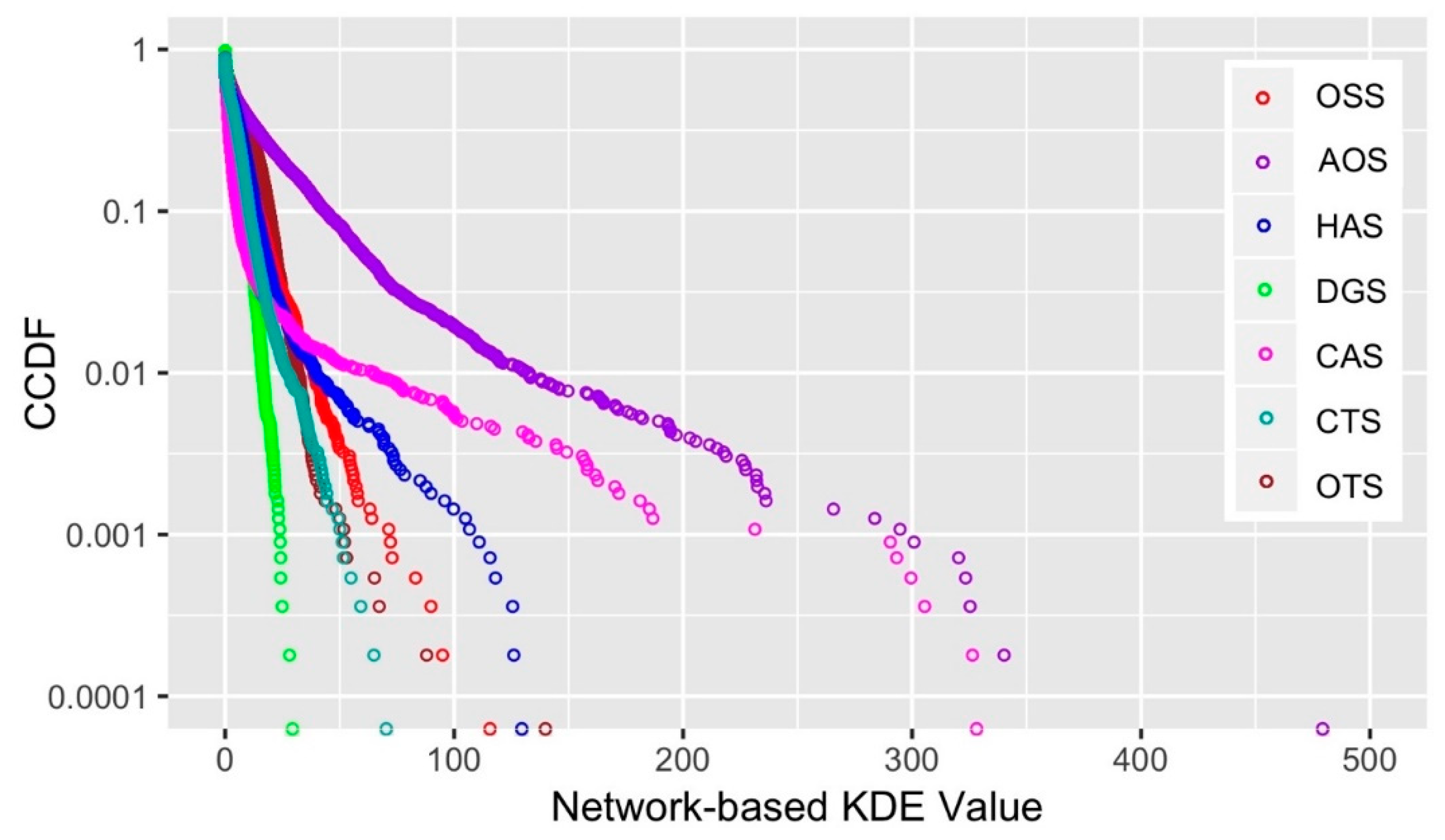
A 2 km bandwidth is used to calculate the NKDE value for all store types. The conditional cumulative distribution function (CCDF) is used to calculate the statistical distribution of the NKDE value. The CCDF indicator, which is defined as , reflects the statistical distribution of samples. The sum of probabilities can be derived when the CCDF value is larger than . Generally, the NKDE value of all store types follows a power-law distribution (Figure 3), referring to the fact that the number of roads decreases geometrically with the increase of the NKDE value. Among all store types, the SS has the longest tail, which indicates that it involves more roads due to its dense distribution. On the contrary, the DS has the shortest tail. A similar power-law distribution has been observed in seven SS subtypes, among which the AOS has the longest tail, and the DGS has the shortest tail (Figure 4).
4.2. Network-Based Spatial Patterns of Retail Stores
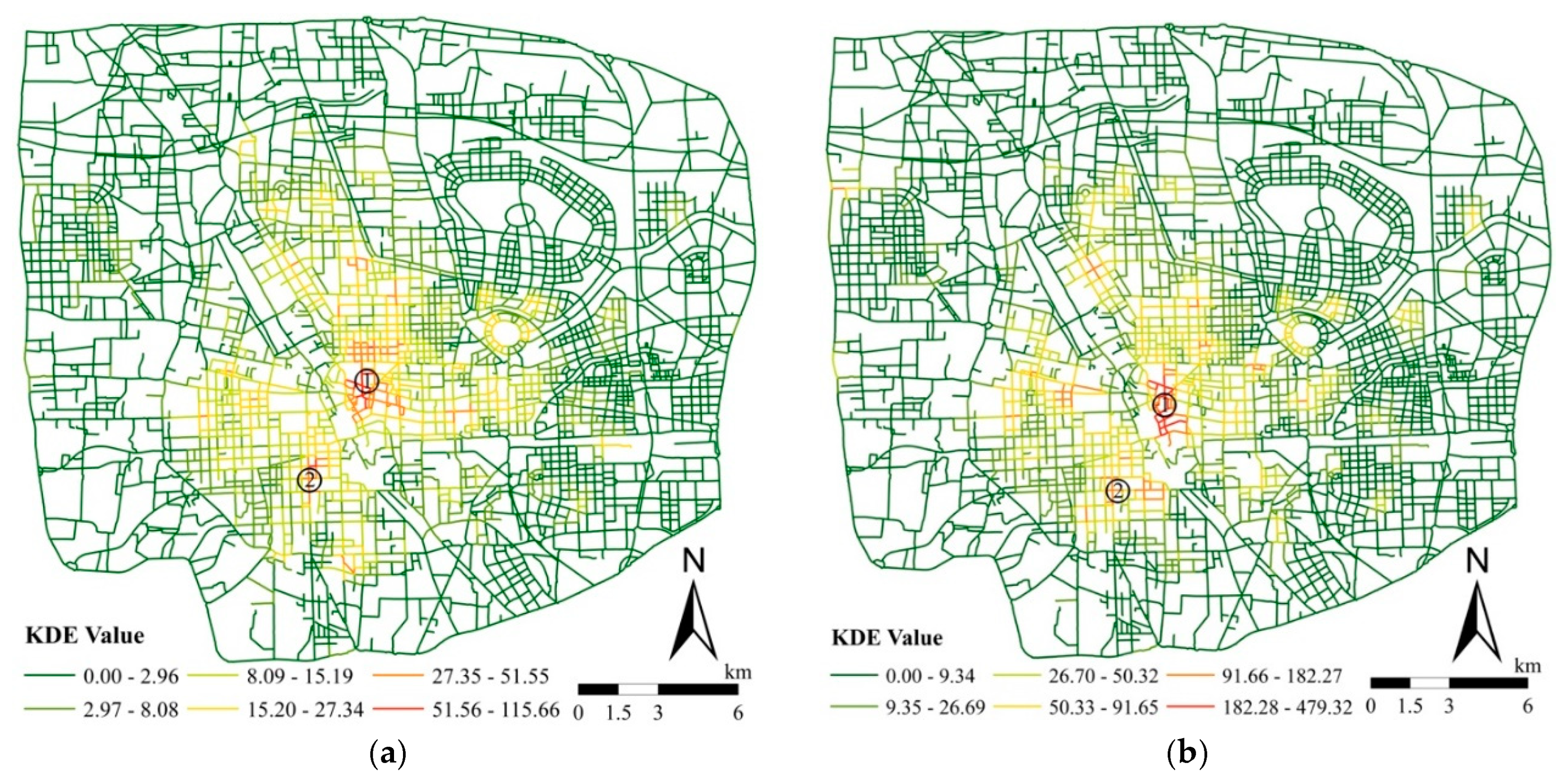
The method described in Section 2.1 is used to calculate the density value of each line cell. The calculation is based on each line cell. It retrieves the point events on all line cells within a given bandwidth range (measured by the network distance) and calculates the corresponding kernel density value through the kernel function. Then, the line cell length is used as the weight to derive the line density, as shown in Figure 5, Figure 6 and Figure 7. In the figures, the NKDE value of a store type represents the concentration of the stores on the road. The NKDE is visually divided into six classes based on the Jenks natural breaks. All stores in the study area are mainly distributed between West 3rd Ring road, Lianyungang-Khorgos Highway, Zhongzhou Avenue, and South 3rd Ring Road (Figure 5). They are concentrated most densely in the Erqi Square near the Zhengzhou Railway Station (position ① in Figure 5). As a traditional business center of Zhengzhou city, this area embodies many large shopping malls. A large number of furniture and home appliance stores are located in the area adjacent to Weilai Road, Zhongzhou Avenue, Zhengbian Road, and Longhai Expressway (position ② in Figure 5). Additionally, many stores are concentrated in the area to the east of Huayuan Road, West of Zhongzhou Avenue, and North of Sanquan Road (position ③ in Figure 5), and at the intersection of Zhongzhou Avenue and South 3rd Ring Road (position ④ in Figure 5). We also performed the network-based KDE for the six store types (Figure 6) and the seven SS subtypes (Figure 7). Table 2 shows the statistical results of the road KDE values for these stores.
4.3. Correlations between NKDE and Closeness Centrality
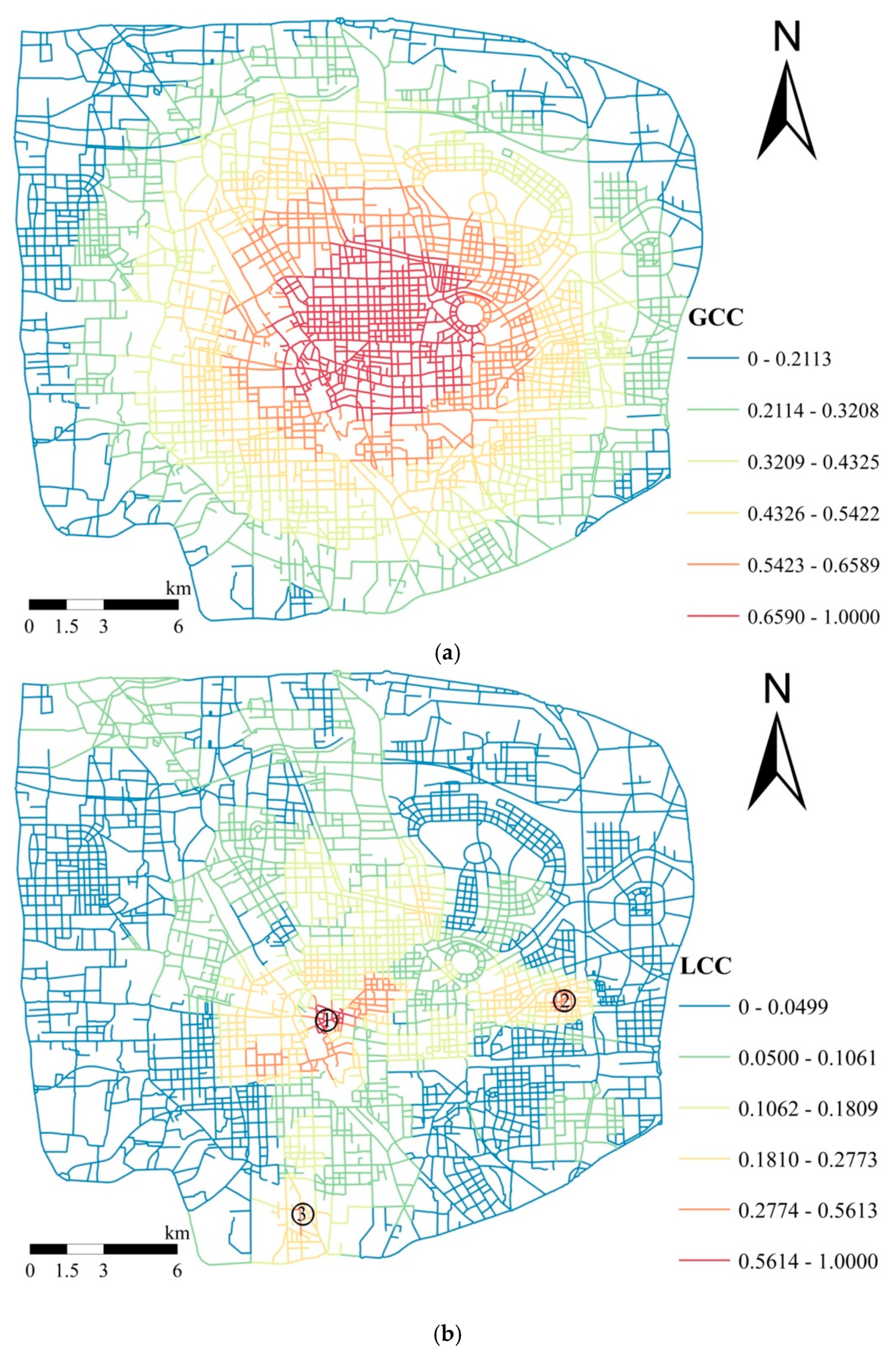
We calculated the GCC, LCC, and WCC values in the study area (Figure 8). The definition of the neighborhood in the LCC calculation is the road network community generated by the Combo algorithm (Figure 2). The closeness centrality manifests a significant level of spatial heterogeneity. The higher the closeness centrality value of a road is, the shorter the road’s average distance to other roads. The GCC represents the average road distance, which gradually decreases from the city center to the periphery (Figure 8a). However, the LCC shows the average distance in a subnetwork and identifies a road with high centrality in a local area. Unlike GCC, there are many local areas with a high LCC value. The old town area surrounding the Zhengzhou East Railway Station has the highest value (position ① in Figure 8b). The roads near the Zhengzhou East Railway Station (position ② in Figure 8b) and the roads between the Zhengping Highway and Daxue South Road (position ③ in Figure 8b) also have high LCC values. The WCC shows both the average distance of the global road network and local subnetworks. Roads with a high WCC value are mainly distributed near the railway station in the old town area. The roads near Erqi Square have the highest WCC value, which means that those roads have a considerable level of accessibility to all other roads in the network.
The correlation coefficient between the NKDE value and the closeness centrality is also calculated, as shown in Table 3. Among the six store types, SS and SMS have the highest level of correlation, meaning that they are relatively accessible to all other nodes and have considerable potential to attract customers. In particular, the high correlation coefficient is shown between SS and WCC, between SS and GCC, as well as between SS and LCC. This is very likely due to the location advantage of SS, which are normally distributed in the center of the subnetworks. However, the FS and CMS show a low level of correlation. This result is due to the relatively few stores covering a large serve area: Because of their relative sensitivity to land lease, these stores are generally located in the urban fringe.
To examine the effects of different bandwidths in the NKDE, three bandwidths, including 0.5-km, 1 km, and 2 km, were implemented. Then, we compared the correlation with GCC, LCC, and WCC with these three bandwidths (Figure 9). The results show a positive correlation coefficient for all bandwidths except CAS; however, the correlation coefficient is comparatively small under a small bandwidth. For example, the correlation coefficient between SS and WCC decreases from 0.58 to 0.48, and that between OSS and WCC decreases from 0.63 to 0.48. However, the difference between different bandwidths is not significant.
4.4. Discussion
Spatial distribution and location analysis of business retailers have been the focus of urban planning and business administration. Most existing studies used regular grid cells or administrative units to perform spatial analysis. These analyses suffer considerably from statistical biases, such as the MAUP and the edge effect. These methodological caveats are addressed in the paper using a network-based analysis. The correlation analysis between the store density and the street closeness centrality are also discussed. The results show various levels of correlation by store type.
Specifically, in a road network, the node with the highest level of closeness centrality value will always stay close to the geometric center of the network [62,63]; the higher the closeness centrality of a road is, the shorter its average distance to other roads and the better its accessibility. In the study area, the index of GCC shows a circular distribution similar to concentric circles in space, while LCC shows a similar distribution in each subnetwork (Figure 8). We can see that the closeness centrality represents the distance between a node and the centroid of the network: The higher the closeness centrality is, the closer the node to the centroid of the network. As nodes in a network do not distribute evenly, the centroid does not entirely coincide with the geometric center of the network. Therefore, in actual road networks, the centroids reflected by the closeness centrality can characterize the kernel of a city or the network-based centroid. The irregular concentric spatial circles in the distribution are able to indicate the city structure kernel. Furthermore, stores with a high LCC correlation tend to distribute in the center of the subnetwork. In reality, such stores tend to have relative accessibility and are able to attract passing traffic and customers, thus helping to gain a business potential and achieve sustainable development.
The methods and findings of the paper can provide valuable insights into urban planning. By analyzing the correlation between the facility distribution and the closeness centrality of urban road networks, it is possible to optimize the spatial patterns of the commercial facilities. For example, results drawn from the study suggest that future planning strategies could include relocating part of the facilities, such as those with a high demand for space but low sensitivity to travel distance, to the urban fringe. In addition, the identification of a city’s sub-centers will help to delineate the city’s polycentric spatial structure, providing evidence for taking future planning initiatives.
Physical accessibility is a crucial factor for the location strategy of retailers. The results of the correlation analysis using the network struture is consistent with similar analyses in other case studies, including Bologna [13], Barcelona [14], Changchun [15], and Guangzhou [16], all of which used a grid cell structure. These studies confirm the hypothesis that street centrality is a crucial feature in the urban structure and land-use pattern and also indicate that commercial retail market tends to be concentrated in areas with better centrality. Results derived from the store subtypes could be compared with these studies and are significant for capturing trends and strategies of urban development in different cities. For example, in the study area, the correlation between CPS and GCC is higher than that between DS and GCC. In Changchun, a northeastern Chinese city, the conclusion is the opposite [15]. This observation is mainly attributed to the development strategy of the Zhengdong New District in the study area. The new development in the district is separate from expanding the old town center. It aims to establish a suburban center by following the future development goals outlined in the planning blueprint of Zhengzhou City 2010–2030. This development plan has encouraged the establishment of large shopping centers (i.e., DS in the analysis) in the new suburban center and can be identified by the global correlation coefficient (e.g., between DS and GCC). It can be observed from the analysis that urban planning and development policies differ across cities and could largely influence the spatial structure of the retail industry. These patterns could be identified using the network-based analysis as exemplified in the paper.
The correlation difference between the network-based and cell-based KDE (CKDE) are compared. Firstly, the CKDE for various commercial POI and three closeness centralities are calculated based on 100 m grid cells, and then correlation analysis is conducted (Table 4, Figure 10, Figure 11 and Figure 12). The bandwidth of the CKDE is set to 2 km. It is illustrated that the correlation coefficients with the two types of the KDE are generally consistent in the distribution trends for different store types, but the correlation coefficient based on the CKDE is higher than that of the NKDE. This result is attributed to the smoothing effect of the CKDE as the small difference in density values between adjacent cells in the CKDE calculation. In fact, since retail stores has most points distributed along the street, the NKDE better reveals its spatial distribution pattern.
This study also has limitations. First, there are methodological caveats in the analysis. For example, the paper employs the closeness centrality of the network to measure the network structure while ignoring other network metrics. In the process of closeness centrality calculation, the shortest path algorithm only takes into account the distance metric and fails to consider the hierarchical structure of the road network, such as the speed limit. In the calculation of the KDE, the bandwidth parameter should be optimized using fitted models. Second, the identification of the spatial pattern is only focused on the supply side (i.e., POI data) while ignoring the demand or the consumers’ need. Future analysis of the retailer accessibility can employ spatial interaction models, such as the two-step floating catchment area method [18]. Third, the distribution of commercial POI is influenced by factors separate from the transport infrastructure, such as commuting population and land use. Thus, it is necessary to weight in these factors using other spatial measures such as the geographically weighted regressing method. Lastly, the study only considers the brick-and-mortar stores and disregards other retail forms, especially online retailers. How to evaluate the impact of the internet retailer on urban development with cutting edge spatial methods would be an area worthy of further exploration.
5. Conclusions
Identifying the spatial pattern of urban retailers is valuable for understanding land use and business potential of a city. In this paper, the store density is modeled using a network structure and quantified by network metrics. Correlations between the store density and the network closeness centrality are discussed based on both the global and local effects across different store types. The paper also derives the store density by store type and subtype using the NKDE method. Three closeness centrality indicators (i.e., GCC, LCC, and WCC) are proposed to gauge the spatial pattern and are correlated with the NKDE. Further analysis indicates that stores with a high correlation tend to be distributed in either the city center (i.e., GCC) or the subnetwork center (i.e., LCC). Retail stores located on these roads have a relative location advantage and have the potential to attract passing traffic and customers. These findings can provide suggestions to optimize the spatial pattern of commercial facilities and are valuable for promoting the sustainable development of the city.
Author Contributions
Z.H. designed and performed the experiments and wrote this paper. C.C. designed the experiments and analyzed the data. C.M. supervised the implementation of the project. H.W. contributed data collection and analysis. X.C. edited the manuscript.
Funding
This research was funded by National Natural Science Foundation of China, grant number 41601116 and 41871316; Key Project of Humanities and Social Sciences by Key Research Base of the Ministry of Education, China, Grant number 16JJD770019; Science and Technology Foundation of Henan Province, grant number 172102110286; and the Henan University Science Foundation for Young Talents.
Acknowledgments
Special thanks go to the editor and anonymous reviewers of this paper for their constructive comments.
Conflicts of Interest
The authors declare no conflict of interest.
References
- Barry, R.B.; Joel, R.E.; Patrali, M.C. Retail Management: A Strategic Approach, 13th ed.; Pearson Education: Harlow, UK, 2018; pp. 22–42. [Google Scholar]
- Glaeser, E.L.; Kolko, J.; Saiz, A. Consumer city. J. Econ. Geogr. 2001, 1, 27–50. [Google Scholar] [CrossRef]
- Wang, S. China’s New Retail Economy: A Geographic Perspective; Routledge: New York, NY, USA, 2014; pp. 10–60. [Google Scholar]
- Goldman, A. The transfer of retail formats into developing economies: The example of China. J. Retail. 2001, 77, 221–242. [Google Scholar] [CrossRef]
- Thomas, W.; Susan, G.M. Retail gravitation and economic impact: A market-driven analytical framework for bike-share station location analysis in the United States. Int. J. Sustain. Transp. 2016, 10, 247–259. [Google Scholar]
- Les, D.; Michalis, P.; Alex, S. Estimating attractiveness, hierarchy and catchment area extents for a national set of retail centre agglomerations. J. Retail. Consum. Serv. 2016, 28, 78–90. [Google Scholar] [Green Version]
- Michael, F.G. LACS: A Location-Allocation Mode for Retail Site Selection. J. Retail. 1984, 60, 84–100. [Google Scholar]
- Norat, R.T.; Amparo, B.P.; Juan, B.V.; Francisco, M.V. The retail site location decision process using GIS and the analytical hierarchy process. Appl. Geogr. 2013, 40, 191–198. [Google Scholar]
- Mike, G. The Poetics of Cities: Designing Neighborhoods That Work; The Ohio State University Press: Columbus, OH, USA, 1995; pp. 1–16. [Google Scholar]
- Michael, F.D. The geometry of central place theory. Geogr. Ann. B 1965, 47, 111–124. [Google Scholar]
- Gordon, F.M. Agglomeration and central place theory: A review of the literature. Int. Reg. Sci. Rev. 1984, 9, 1–42. [Google Scholar]
- Guy, C. The Retail Development Process. Location, Property and Planning; Routeledge: London, UK, 1994; pp. 12–36. [Google Scholar]
- Sergio, P.; Emanuele, S.; Valentino, I.; Roberto, M.; Vito, L.; Alessio, C.; Wang, F.H.; Salvatore, S. Street centrality and densities of retail and services in Bologna, Italy. Environ. Plan. B 2009, 36, 450–465. [Google Scholar]
- Sergio, P.; Vito, L.; Wang, F.H.; Salvador, R.; Emanuele, S.; Salvatore, S.; Alessio, C.; Eugenio, B.; Francisco, C.; Berta, C. Street centrality and the location of economic activities in Barcelona. Urban Stud. 2012, 49, 1471–1488. [Google Scholar]
- Wang, F.H.; Chen, C.; Xiu, C.L.; Zhang, P.Y. Location analysis of retail stores in Changchun, China: A street centrality perspective. Cities 2014, 41, 54–63. [Google Scholar] [CrossRef]
- Lin, G.; Chen, X.X.; Liang, Y.T. The location of retail stores and street centrality in Guangzhou, China. Appl. Geogr. 2018, 100, 12–20. [Google Scholar] [CrossRef]
- He, S.W.; Yu, S.; Wei, P.; Fang, C.L. A spatial design network analysis of street networks and the locations of leisure entertainment activities: A case study of Wuhan, China. Sustain. Cities Soc. 2019, 44, 880–887. [Google Scholar] [CrossRef]
- Chen, X. Take the edge off: A hybrid geographic food access measure. Appl. Geogr. 2017, 87, 149–159. [Google Scholar] [CrossRef]
- Matthew, C.; Steve Ti Tim, H.; Taner, O. Public Places Urban Spaces, The Dimensions of Urban Design, 2nd ed.; Routledge: New York, NY, USA, 2012; pp. 180–190. [Google Scholar]
- Jacobs, J. The Death and Life of Great American Cities: The Failure of Town Planning; Random House: New York, NY, USA, 1961; pp. 1–25. [Google Scholar]
- Stephen, M. Streets and Patterns; Routledge: New York, NY, USA, 2005; pp. 235–258. [Google Scholar]
- Shen, Y.; Kayvan, K. Urban function connectivity: Characterisation of functional urban streets with social media check-in data. Cities 2016, 55, 9–21. [Google Scholar] [CrossRef] [Green Version]
- Okabe, A.; Okunuki, K. A computational method for estimating the demand of retail stores on a street network and its implementation in GIS. Trans. GIS 2001, 5, 209–220. [Google Scholar] [CrossRef]
- Hillier, B.; Hanson, J. The Social Logic of Space; Cambridge University Press: London, UK, 1989; pp. 1–32. [Google Scholar]
- Hillier, B. Space Is the Machine: A Configurational Theory of Architecture; Space Syntax: London, UK, 2007; pp. 21–52. [Google Scholar]
- Itzhak, O.; Ran, G. Spatial patterns of retail activity and street network structure in new and traditional Israeli cities. Urban Geogr. 2016, 37, 629–649. [Google Scholar]
- Wang, F.H.; Antipova, A.; Sergio, P. Street centrality and land use intensity in Baton Rouge, Louisiana. J. Transp. Geogr. 2011, 19, 285–293. [Google Scholar] [CrossRef] [Green Version]
- Wang, S.; Xu, G.; Guo, Q.S. Street Centralities and Land Use Intensities Based on Points of Interest (POI) in Shenzhen, China. ISPRS. Int. J. Geo-Inf. 2018, 7, 425. [Google Scholar] [CrossRef]
- Kevin, L. The Image of the City; MIT Press: Boston, MA, USA, 1960; pp. 1–26. [Google Scholar]
- Ian, S.; Nikhil, N.; Carlo, R.; Raphäel, P. Green streets− Quantifying and mapping urban trees with street-level imagery and computer vision. Landsc. Urban Plan. 2017, 165, 93–101. [Google Scholar]
- Li, X.J.; Zhang, C.R.; Li, W.D.; Robert, R.; Meng, Q.Y.; Zhang, W.X. Assessing street-level urban greenery using Google Street View and a modified green view index. Urban For. Urban Green. 2015, 14, 675–685. [Google Scholar] [CrossRef]
- Long, Y.; Liu, L. How green are the streets? An analysis for central areas of Chinese cities using Tencent Street View. PLoS ONE 2017, 12, e0171110. [Google Scholar]
- Gong, F.Y.; Zeng, Z.C.; Zhang, F.; Li, X.J.; Edward, N.; Leslie, K.N. Mapping sky, tree, and building view factors of street canyons in a high-density urban environment. Build. Environ. 2018, 134, 155–167. [Google Scholar] [CrossRef]
- Yin, Y.; Wang, Z.X. Measuring visual enclosure for street walkability: Using machine learning algorithms and Google Street View imagery. Appl. Geogr. 2016, 76, 147–153. [Google Scholar] [CrossRef]
- Li, X.J.; Carlo, R.; Ian, S. Quantifying the shade provision of street trees in urban landscape: A case study in Boston, USA, using Google Street View. Landsc. Urban Plan. 2018, 169, 81–91. [Google Scholar] [CrossRef]
- Li, X.J.; Carlo, R. Mapping the spatio-temporal distribution of solar radiation within street canyons of Boston using Google Street View panoramas and building height model. Landsc. Urban Plan. 2018. [Google Scholar] [CrossRef]
- Hao, J.W.; Zhu, J.; Zhong, R. The rise of big data on urban studies and planning practices in China: Review and open research issues. J. Urban Manag. 2015, 4, 92–124. [Google Scholar] [CrossRef] [Green Version]
- Zhu, D.; Wang, N.H.; Wu, L.; Liu, Y. Street as a big geo-data assembly and analysis unit in urban studies: A case study using Beijing taxi data. Appl. Geogr. 2017, 86, 152–164. [Google Scholar] [CrossRef]
- Wu, L.; Zhi, Y.; Sui, Z.W.; Liu, Y. Intra-urban human mobility and activity transition: Evidence from social media check-in data. PLoS ONE 2014, 9, e97010. [Google Scholar] [CrossRef]
- Pucci, P.; Fabio, M.; Paolo, T. Mapping Urban Practices through Mobile Phone Data; Springer: Berlin, Germany, 2015; pp. 21–70. [Google Scholar]
- Yuan, J.; Zheng, Y.; Xie, X. Discovering regions of different functions in a city using human mobility and POIs. In Proceedings of the 18th ACM SIGKDD International Conference on Knowledge Discovery and Data Mining, Beijing, China, 12–16 August 2012; pp. 1–9. [Google Scholar]
- Gao, S.; Janowicz, K.; Couclelis, H. Extracting urban functional regions from points of interest and human activities on location-based social networks. Trans. GIS 2017, 21, 446–467. [Google Scholar] [CrossRef]
- Hu, T.Y.; Yang, J.; Li, X.C.; Gong, P. Mapping urban land use by using landsat images and open social data. Remote Sens. 2016, 8, 151. [Google Scholar] [CrossRef]
- Liu, X.P.; He, J.L.; Yao, Y.; Zhang, J.B.; Liang, H.L.; Wang, H.; Hong, Y. Classifying urban land use by integrating remote sensing and social media data. Int. J. Geogr. Inf. Sci. 2017, 31, 1675–1696. [Google Scholar] [CrossRef]
- Biłozor, A.; Kowalczyk, A.M.; Bajerowski, T. Theory of Scale-Free Networks as a New Tool in Researching the Structure and Optimization of Spatial Planning. J. Urban Plan. Dev. 2018, 144, 04018005. [Google Scholar] [CrossRef]
- Kowalczyk, A.M. The analysis of networks space structures as important elements of sustainable space development. In Proceedings of the International Conference on Environmental Engineering, Saulėtekio, Lithuania, 27–28 April 2017; pp. 1–6. [Google Scholar]
- Xie, Z.X.; Yan, J. Kernel density estimation of traffic accidents in a network space. Comput. Environ. Urban Syst. 2008, 32, 396–406. [Google Scholar] [CrossRef]
- Christopher, L. Spatial Data Analysis: An Introduction for GIS Users; Oxford University Press: London, UK, 2010; pp. 102–169. [Google Scholar]
- Tang, L.L.; Kan, Z.H.; Zhang, X.; Sun, F.; Xue, Y.; Li, Q.Q. A network Kernel Density Estimation for linear features in space–time analysis of big trace data. Int. J. Geogr. Inf. Sci. 2016, 30, 1717–1737. [Google Scholar] [CrossRef]
- Okabe, A.; Kokichi, S. Spatial Analysis along Networks: Statistical and Computational Methods; John Wiley & Sons: Chichester, UK, 2012; pp. 171–190. [Google Scholar]
- She, B.; Zhu, X.Y.; Ye, X.Y.; Guo, W.; Su, K.H.; Jay, L. Weighted network Voronoi Diagrams for local spatial analysis. Comput. Environ. Urban Syst. 2015, 52, 70–80. [Google Scholar] [CrossRef]
- Stanley, W.; Katherine, F. Social Network Analysis: Methods and Applications; Cambridge University Press: Cambridge, UK, 1994; pp. 1–35. [Google Scholar]
- Linton, C.F. Centrality in social networks conceptual clarification. Soc. Netw. 1978, 1, 215–239. [Google Scholar]
- Emanuele, S.; Matheus, V.; Luciano, F.C.; Alessio, C.; Sergio, P.; Vito, L. Urban street networks, a comparative analysis of ten European cities. Environ. Plan. B 2013, 40, 1071–1086. [Google Scholar]
- Sergio, P.; Paolo, C.; Vito, L. The network analysis of urban streets: A primal approach. Environ. Plan. B 2006, 33, 705–725. [Google Scholar]
- Newman, M.E. Modularity and community structure in networks. Proc. Natl. Acad. Sci. USA 2006, 103, 8577–8582. [Google Scholar] [CrossRef] [Green Version]
- Huang, L.P.; Yang, Y.J.; Gao, H.P.; Zhao, X.H.; Du, Z.W. Comparing Community Detection Algorithms in Transport Networks via Points of Interest. IEEE Access 2018, 6, 29729–29738. [Google Scholar] [CrossRef]
- Stanislav, S.; Riccardo, C.; Alexander, B.; Carlo, R. General optimization technique for high-quality community detection in complex networks. Phys. Rev. 2014, 90, 1–8. [Google Scholar]
- Ghalmane, Z.; El Hassouni, M.; Cherifi, C.; Cherifi, H. Centrality in modular networks. EPJ Data Sci. 2019, 8, 1–27. [Google Scholar] [CrossRef]
- Andres, S.; Michael, M. Urban network analysis: A new toolbox for measuring city form in ArcGIS. In Proceedings of the 2012 Symposium on Simulation for Architecture and Urban Design, Orlando, FL, USA, 26–29 March 2012; pp. 1–15. [Google Scholar]
- Wang, X.F.; John, T. Zhengzhou—Political economy of an emerging Chinese megacity. Cities 2019, 84, 104–111. [Google Scholar] [CrossRef]
- Jiang, B. Street hierarchies: A minority of streets account for a majority of traffic flow. Int. J. Geogr. Inf. Sci. 2009, 23, 1033–1048. [Google Scholar] [CrossRef]
- Alexander, E.; Michael, L.; Kay, W.A. Graph-theoretical analysis of the Swiss road and railway networks over time. Netw. Spat. Econ. 2009, 9, 379–400. [Google Scholar]
Figure 1.
Result of the community detection in the study area. The road network is divided into 30 network-based communities by the Combo algorithm.
Figure 1.
Result of the community detection in the study area. The road network is divided into 30 network-based communities by the Combo algorithm.

Figure 2.
Road networks of Zhengzhou, China (2018).

Figure 3.
The conditional cumulative distribution function (CCDF) of the network-based kernel density estimation (NKDE) value for six store types.
Figure 3.
The conditional cumulative distribution function (CCDF) of the network-based kernel density estimation (NKDE) value for six store types.

Figure 4.
CCDF of the NKDE value for seven SS subtypes.

Figure 5.
Network-based KDE value for all retail stores.

Figure 6.
Network-based KDE value for six store types. (a) SS; (b) DS; (c) SMS; (d) FS; (e) CMS; (f) CPS.
Figure 6.
Network-based KDE value for six store types. (a) SS; (b) DS; (c) SMS; (d) FS; (e) CMS; (f) CPS.


Figure 7.
Network-based KDE value of six SS subtypes. (a) OSS; (b) AOS; (c) HAS; (d) DGS; (e) CAS; (f) CTS.
Figure 7.
Network-based KDE value of six SS subtypes. (a) OSS; (b) AOS; (c) HAS; (d) DGS; (e) CAS; (f) CTS.


Figure 8.
The closeness centrality of roads in the study area. (a) GCC; (b) LCC; (c) WCC.


Figure 9.
Correlations between the NKDE value and the closeness centrality with different bandwidth. * and ** represent a significance level of 0.1 and 0.01, respectively; # represents non-significance; other significance levels are at 0.001.
Figure 9.
Correlations between the NKDE value and the closeness centrality with different bandwidth. * and ** represent a significance level of 0.1 and 0.01, respectively; # represents non-significance; other significance levels are at 0.001.

Figure 10.
The comparison of correlation coefficients with GCC between CKDE and NKDE.

Figure 11.
The comparison of correlation coefficients with LCC between CKDE and NKDE.

Figure 12.
The comparison of correlation coefficients with WCC between CKDE and NKDE.


Table 1.
Descriptive summary of retail stores in the study area.
| Store Type | Store Subtype | Store Count | Road Count | Average Stores Per Street | Line Cell Count | Average Stores Per Line Cell |
|---|---|---|---|---|---|---|
| Specialty stores (SS) | Office supply stores (OSS) | 4285 | 897 | 4.7770 | 1374 | 3.1186 |
| Apparel shop stores (AOS) | 15456 | 1245 | 12.4145 | 1829 | 8.4505 | |
| Home appliance stores (HAS) | 4919 | 1035 | 4.7527 | 1626 | 3.0252 | |
| Drug stores (DGS) | 3142 | 979 | 3.2094 | 1555 | 2.0206 | |
| Car stores (CAS) | 3811 | 434 | 8.7811 | 795 | 4.7937 | |
| Cosmetics stores (CTS) | 3569 | 860 | 4.1500 | 1367 | 2.6108 | |
| Other stores (OTS) | 6587 | 1491 | 4.4178 | 2156 | 3.0552 | |
| Subtotal | 41769 | 2285 | 18.2796 | 3335 | 12.5244 | |
| Department stores (DS) | 249 | 121 | 2.0579 | 179 | 1.3911 | |
| Supermarkets (SMS) | 2377 | 823 | 2.8882 | 1375 | 1.7287 | |
| Furniture stores (FS) | 4211 | 492 | 8.5589 | 803 | 5.2441 | |
| Construction material stores (CMS) | 13271 | 1147 | 11.5702 | 1887 | 7.0329 | |
| Consumer product stores (CPS) | 16900 | 1966 | 8.5961 | 2967 | 5.6960 | |
| All Stores (AS) | 78777 | 2652 | 29.7048 | 3934 | 20.0247 | |
Table 2.
Statistics of network-based KDE values by store type.
| Store Type | Store Subtype | Average | Median | Maximum | Standard Deviation |
|---|---|---|---|---|---|
| Specialty stores (SS) | Office supply stores (OSS) | 6.2003 | 3.2650 | 115.6580 | 8.5152 |
| Apparel shop stores (AOS) | 17.6005 | 6.6483 | 479.3170 | 29.8941 | |
| Home appliance stores (HAS) | 6.1540 | 3.5878 | 129.5320 | 9.3261 | |
| Drug stores (DGS) | 3.8343 | 2.2271 | 29.3573 | 4.1453 | |
| Car stores (CAS) | 4.0902 | 1.1406 | 328.1910 | 16.7913 | |
| Cosmetics stores (CTS) | 4.7676 | 3.1391 | 70.3148 | 5.9746 | |
| Other stores (OTS) | 8.2742 | 5.9976 | 139.8360 | 8.4355 | |
| Subtotal | 40.3303 | 22.3597 | 766.2540 | 52.1403 | |
| Department stores (DS) | 0.3422 | 0.0388 | 11.8333 | 0.8177 | |
| Supermarkets (SMS) | 3.1721 | 2.3872 | 63.3645 | 3.6940 | |
| Furniture stores (FS) | 5.5538 | 1.5317 | 191.4990 | 13.9360 | |
| Construction material stores (CMS) | 14.4089 | 5.1197 | 506.5090 | 35.1740 | |
| Consumer product stores (CPS) | 17.9092 | 12.5695 | 406.3060 | 20.4603 | |
| All Stores (AS) | 74.5491 | 45.1345 | 1105.7300 | 88.6215 | |
Table 3.
The correlation coefficients between store NKDE and street closeness centrality.
| Store Type | Store Subtype | GCC | LCC | WCC |
|---|---|---|---|---|
| Specialty stores (SS) | Office supply stores (OSS) | 0.5602 *** | 0.5938 *** | 0.6309 *** |
| Apparel shop stores (AOS) | 0.4702 *** | 0.5446 *** | 0.5657 *** | |
| Home appliance stores (HAS) | 0.4535 *** | 0.4105 *** | 0.4676 *** | |
| Drug stores (DGS) | 0.5666 *** | 0.3485 *** | 0.4536 *** | |
| Car stores (CAS) | 0.0173 # | −0.0489 *** | −0.0296 * | |
| Cosmetics stores (CTS) | 0.5172 *** | 0.5204 *** | 0.5623 *** | |
| Other stores (OTS) | 0.6166 *** | 0.4669 *** | 0.5626 *** | |
| Subtotal | 0.5391 *** | 0.5284 *** | 0.5790 *** | |
| Department stores (DS) | 0.3367 *** | 0.5049 *** | 0.4856 *** | |
| Supermarkets (SMS) | 0.5344 *** | 0.4564 *** | 0.5290 *** | |
| Furniture stores (FS) | 0.1731 *** | 0.0755 *** | 0.1236 *** | |
| Construction material stores (CMS) | 0.2027 *** | 0.0728 *** | 0.1334 *** | |
| Consumer product stores (CPS) | 0.4432 *** | 0.2722 *** | 0.3568 *** | |
| All Stores (AS) | 0.5322 *** | 0.4542 *** | 0.5265 *** | |
Note: *** significance level of 0.001, * significance level of 0.1, and # not significant.
Table 4.
The correlation coefficients of cell-based KDE between stores and closeness centrality.
| Store Type | GCC | LCC | WCC | |
| SS | OSS | 0.7772 *** | 0.8390 *** | 0.8461 *** |
| AOS | 0.6487 *** | 0.7850 *** | 0.7591 *** | |
| HAS | 0.6842 *** | 0.7001 *** | 0.7339 *** | |
| DGS | 0.7556 *** | 0.6845 *** | 0.7439 *** | |
| CAS | 0.0458 *** | -0.0252 *** | 0.0068 # | |
| CTS | 0.7370 *** | 0.7709 *** | 0.7865 *** | |
| OTS | 0.8251 *** | 0.7482 *** | 0.8187 *** | |
| Subtotal | 0.7381 *** | 0.7914 *** | 0.8041 *** | |
| DS | 0.6354 *** | 0.7740 *** | 0.7395 *** | |
| SMS | 0.8138 *** | 0.7650 *** | 0.8283 *** | |
| FS | 0.3720 *** | 0.2710 *** | 0.3429 *** | |
| CMS | 0.3325 *** | 0.2206 *** | 0.2954 *** | |
| CPS | 0.7055 *** | 0.6189 *** | 0.6874 *** | |
| AS | 0.7383 *** | 0.7128 *** | 0.7630 *** | |
Note: *** significance level of 0.001, # not significant.
© 2019 by the authors. Licensee MDPI, Basel, Switzerland. This article is an open access article distributed under the terms and conditions of the Creative Commons Attribution (CC BY) license (http://creativecommons.org/licenses/by/4.0/).
Share and Cite
MDPI and ACS Style
Han, Z.; Cui, C.; Miao, C.; Wang, H.; Chen, X. Identifying Spatial Patterns of Retail Stores in Road Network Structure. Sustainability 2019, 11, 4539. https://doi.org/10.3390/su11174539
AMA Style
Han Z, Cui C, Miao C, Wang H, Chen X. Identifying Spatial Patterns of Retail Stores in Road Network Structure. Sustainability. 2019; 11(17):4539. https://doi.org/10.3390/su11174539
Chicago/Turabian StyleHan, Zhigang, Caihui Cui, Changhong Miao, Haiying Wang, and Xiang Chen. 2019. "Identifying Spatial Patterns of Retail Stores in Road Network Structure" Sustainability 11, no. 17: 4539. https://doi.org/10.3390/su11174539
Note that from the first issue of 2016, this journal uses article numbers instead of page numbers. See further details here.