1. Introduction
Across the world, urbanization is characterized by the replacement of natural land cover with artificial materials, such as asphalt and concrete, in the form of walls, roofs, and pavements. This leads to the spatial growth of cities and an increase in impervious surfaces, a phenomenon called urban sprawl [
1,
2]. This phenomenon is nearly universal and has been observed in every inhabited continent [
3]. In the United States, Canada, and several other countries, urban sprawl has manifested in the form of growing suburbanization [
4,
5], while the percentage of the population living in the urban core has been declining since the 1950s.
Previous studies have demonstrated the effect of urban sprawl on public health [
6,
7], flora and fauna [
8,
9], air quality [
10], and urban water use [
11,
12,
13]. Another effect of urban sprawl is the development of the Urban Heat Island (UHI) effect. UHI is characterized by urban temperatures which are consistently higher than those in adjacent rural areas. UHI can be studied at various heights, including at the surface (SUHI), the canopy layer (CLUHI), and at the boundary layer (BLUHI) [
14]. Of these, CLUHI, which refers to the air temperature difference 2 m above the ground, is significant because it is the height at which most outdoor activities takes place. In this paper, unless otherwise stated, UHI refers to CLUHI.
The UHI effect at all levels has been extensively documented for decades around the world (see, e.g., [
15,
16,
17,
18,
19] for SUHI and [
20,
21] for UHI at all levels), with the difference in temperatures between urban and adjacent rural areas ranging from less than 1
C (in estimates for Atlanta, USA [
22] for CLUHI) to over 10
C (in estimates for Beijing, China [
16] for SUHI). Memon et al. [
23] summarized the intensity of the UHI, as observed in several studies. The UHI effect is also heterogeneous, varying in both time and space within a city [
24,
25,
26]. Studies have also found that the UHI effect intensifies with increasing urban sprawl [
27,
28,
29], due to the replacement of larger areas of vegetation with artificial surfaces. Ward et al. [
30] examined the relationships between UHI and heat wave episodes in Europe, and found that cities in cooler climates in Northern Europe were actually more susceptible to heat waves. Van Hove [
31] further investigated the spatial and temporal heterogeneity of the UHI effect in the city of Rotterdam in Northern Europe.
A growing number of studies have shown the significance of land cover composition and configuration in affecting near-ground urban air and surface temperatures, highlighting the importance of patch sizes of built environment features. Connors et al. [
32] used high-resolution satellite imagery to investigate the effects of different types of vegetation on land surface temperature. A large area of moisture-intensive vegetation (such as grass) showed a statistically significant effect, whereas more desert-like (xeric) vegetation did not. Zhou et al. [
33] found that spatial composition and configuration of land cover both play a role in UHI mitigation and, so, air temperatures can be decreased not just by increasing the percentage of vegetated surfaces, but also by distributing them optimally. Zhibin et al. [
34] and Zheng et al. [
35] reached a similar conclusion on the composition and configuration of natural and artificial surfaces. Jenerette et al. [
36] examined the relationships between parcel-scale land cover composition and heat-related response on the residents of Phoenix, USA. They found that parcel-scale daytime surface temperatures were correlated with heat-related illnesses. Li et al. [
37] analyzed two blocks of about 500 residential neighborhoods, both in Phoenix, and found that land configuration played a more important role than composition in explaining differences in surface temperatures. Du et al. [
38] studied land cover configuration in Shanghai, China and found that large areas of impervious surfaces had led to an increase in UHI. They recommended that impervious surfaces be interspersed with vegetated surfaces and water bodies to decrease local temperatures.
Oke [
39] established that the UHI effect is caused by changes of the energy balance in the urban boundary layer, with more sensible heat flux than latent heat flux as compared to rural areas. This highest sensible heat flux leads to higher air temperatures. Another study by Oke [
40] showed that UHI intensity increases with the population of a city, which has been confirmed by subsequent studies [
41,
42]. Kleerekoper et al. [
43] listed seven reasons for the UHI effect in urban areas, which included the creation of artificial surfaces that absorb and store more heat than natural surfaces, reduction in evapotranspiration, and a reduced rate of heat exchange due to decreased wind speed, among others. Deilami [
19] analyzed 75 studies to conclude that the most common factors associated with UHI include vegetation cover, season, impervious surfaces, and population density. Phelan et al. [
44] reviewed various studies, explaining the mechanisms and implications of UHI, as well as potential remedies. Previous studies have looked at the role of pavements in increasing the UHI effect [
45,
46,
47,
48]. Typical pavements have a lower solar reflectance (albedo) and a higher thermal diffusivity as compared to natural surfaces, which cause them to absorb and store more heat. This, in turn, heats the surrounding air and generates the UHI effect.
As a result, several studies have suggested using ’cool’ reflective surfaces with higher albedo to decrease the surface temperature. These surfaces include both cool roofs [
49,
50,
51,
52,
53,
54] and cool pavements [
55,
56,
57,
58,
59]. Synnefa et al. [
60] conducted a numerical evaluation of the benefits of the large-scale deployment of reflective surfaces in Athens, Greece and found a potential reduction of ambient air temperatures by up to 2
C. Another study by Georgiakis et al. [
61], also in Athens, suggested a more moderate decrease in ambient air temperature, of about 1
C, although only for a single urban canyon. Carnielo and Zinzi [
62] conducted a study in Rome with reflective asphalt paving materials and found a peak summertime decrease in air temperature of 5.5
C. In comparison, Toparlar [
63] showed that a park inside an urban area in Antwerp could reduce the air temperature by 0.9
C, as compared to a nearby paved area without a park. These studies showed that the UHI within a city is highly variable, being affected by local land-use patterns. Similarly, Allergini et al. [
64] showed that the relative configuration of buildings and roads affects both the wind speed and air temperature at a microscale in urban areas.
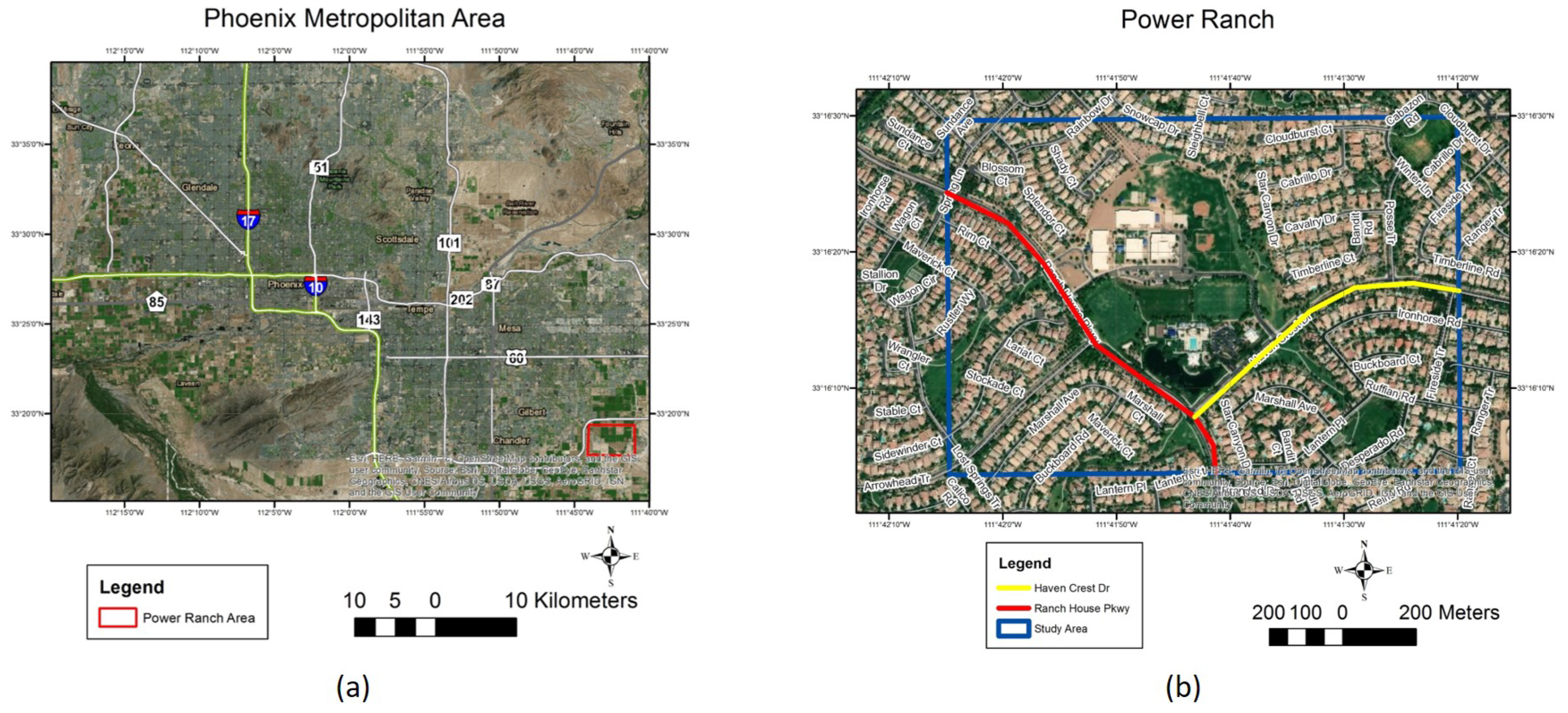
The present study investigates the potential benefits of using cool surfaces to mitigate UHI in the Power Ranch community in the Phoenix Metropolitan Area in Arizona, USA. This metropolitan area has been growing for decades, covering an increasingly larger area with paved materials interspersed with different types of vegetation. It has also been the subject of a number of UHI-related investigations. Middel et al. [
65] investigated the interaction between local urban forms and different types of vegetation on air temperatures with a numerical model, and concluded that a smart mix of urban form and landscaping options could mitigate the UHI during daytime hours. Golden and Kaloush [
45] investigated the albedo of pavements in Phoenix. They showed experimentally that increasing the albedo by using simple white paint sprayed on to a test section could significantly reduce the daytime surface temperature and, hence, the UHI. Yang and Kaloush [
66] investigated the potential of using reflective pavements in the Phoenix area to mitigate the UHI. They used the Weather Research and Forecasting (WRF) model to determine the 2 m air temperature at a characteristic length scale of over 1 km (mesoscale). This type of modeling did not explain the effect of the reflective surfaces on individual buildings and neighborhoods below the 1 km scale (i.e., at a microscale). As the previous literature has shown, land cover composition and configuration has a significant effect on UHI, and typical urban and suburban areas tend to have changes in their land cover over short distances (such as grassy areas next to roads and sidewalks). Thus, a microscale approach is necessary to quantify local benefits of cool surfaces.
The present study addresses two research questions:
How can a Computational Fluid Dynamics (CFD) model be developed and validated to determine the microscale 2 m air temperature throughout a relatively small area with heterogeneous land cover?
To what extent can 2 m air temperature during summertime peak afternoon periods be decreased in this area, both upstream and downstream of the prevailing wind, by using reflective surfaces?
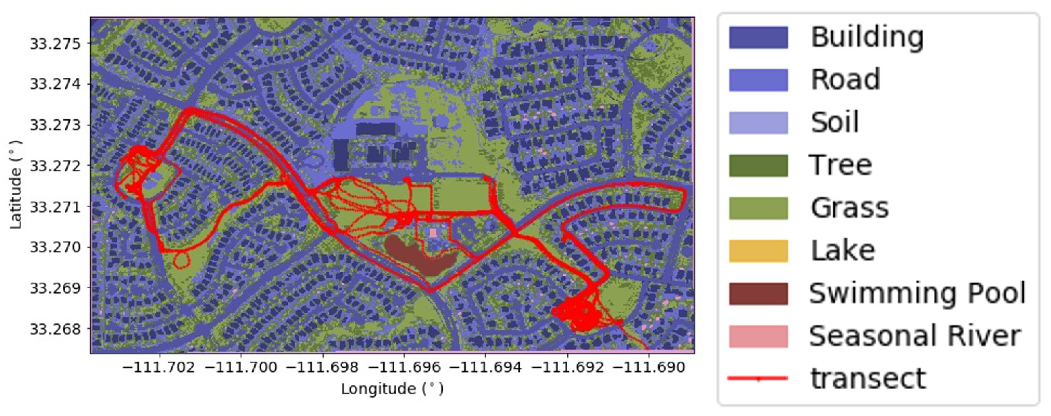
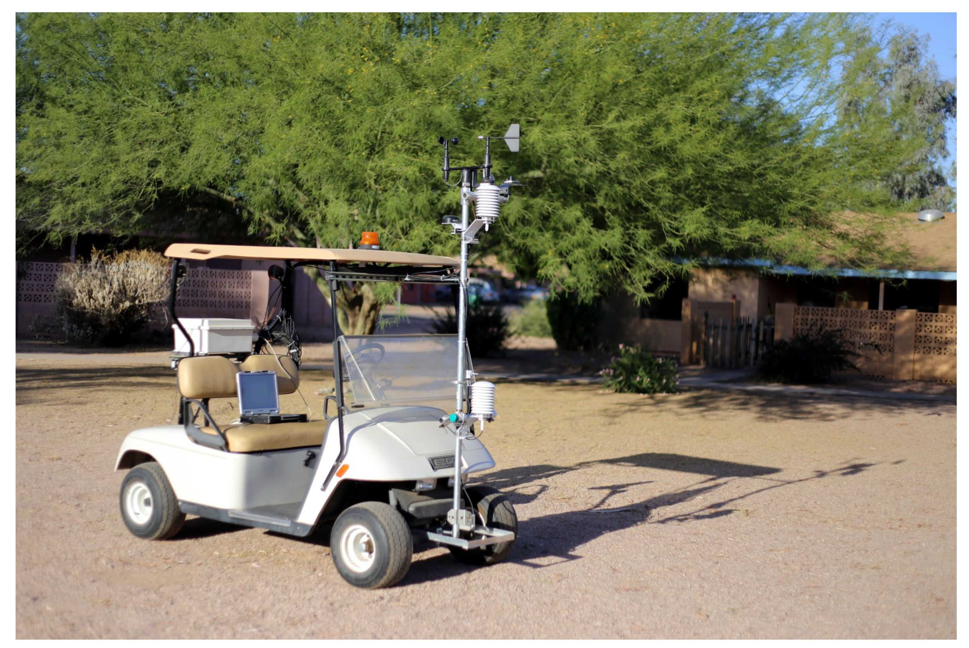
These two questions were investigated through a case study in the Power Ranch community in Arizona, USA. The area was investigated using meteorological data collected on 13 August 2015 between 5:00 p.m. and 6:00 p.m. using a mobile platform to build a validated CFD model of the local microclimate, and then use that model to study the effects of reflective surfaces. A validated, microscale CFD model has not previously been developed for this area, and its particular land cover configuration make it a novel investigation for the effectiveness of reflective surfaces. This study shows how engineers and urban planners can develop local models for individual neighborhoods and cities to better plan for UHI mitigation.
4. Model Development
In order to create a validated model of the effect of pavements on the urban microclimate, an uncoupled pavement-urban canyon model was adapted from a previous study [
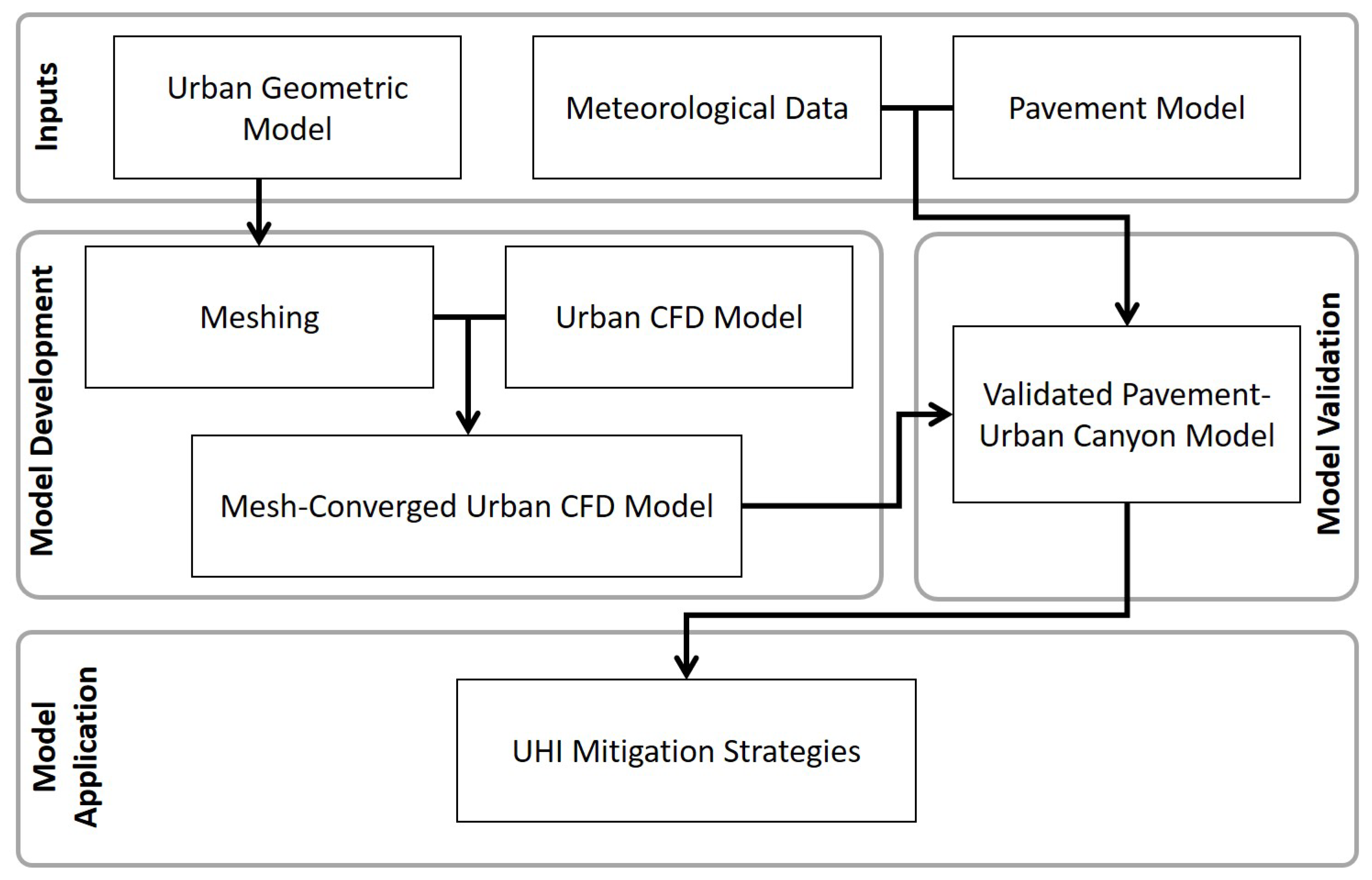
78] and validated for the current one. This validated model was then used to study the effect of cool pavements. The steps used to develop, validate, and then use the model are summarized in
Figure 4. The modeling effort consisted of two sub-models: A pavement model, which used a one-dimensional numerical method to calculate the surface temperature of pavements in the urban area; and a three-dimensional Computational Fluid Dynamics (CFD)-based urban canyon model to calculate the air temperature. The variable of interest was the 2 m air temperature, which corresponds to the Canopy Layer UHI. This is important, as most outdoor human activity takes place at this height and, so, it has the most significant impact on urban areas.
As a first step towards validation of the existing model framework with the Power Ranch neighborhood location and features, the model results were compared with the measured 2 m air temperature, surface temperature, and wind speed data collected over the roads. The following subsections describe the model and its validation. The model was evaluated for data collected between 5:00 and 6:00 p.m. on 13 August 2015. The relative humidity (RH) was not included in the model, as the average RH measured at 2 m during the study period was very low (about 10–20%), which would have only a minor impact on the 2 m air temperature. Although RH is an important variable for human comfort, this study was restricted to 2 m air temperature and, thus, RH was outside its scope.
4.1. Pavement Model
The pavement model used was a one-dimensional finite volume heat transfer model, called ILLI-THERM, which accounts for absorbed solar radiation at the surface (which, in turn, depends on the albedo, the geographical location of the study area, and the time), loss of energy through convection and radiation, and the movement of thermal energy through various pavement layers. Details of the model can be found in [
47].
Information about the pavement thickness and properties were not available, but the transect measurements showed that the average road surface temperature during the hour of study was 50.35
C. The properties shown in
Table 2 were assumed, as those of typical aged asphalt pavements used for local streets, as measured in a previous study [
75], together with a far-field wind speed of 0.45 m/s and air temperature of 42.22
C, which were obtained from the nearby (about 10 km away) Phoenix-Mesa Gateway Airport weather station on the hour of analysis.
Using these properties, the calculated surface temperature of the road was 50.22 C, which is very similar to the average measured value. Thus, these properties were used for the pavement model.
4.2. Urban Canyon Model
The urban canyon model used was a three-dimensional CFD model that numerically solves the Reynold’s Average Navier Stokes (RANS) equations, implemented on the open-source CFD solver OpenFOAM [
79]. The model consists of the RANS continuity equation shown in Equation (
1), the RANS momentum equation shown in Equation (
2), and the RANS energy equation shown in Equation (
3), where
is the RANS velocity component along the
direction (
),
P is the kinematic pressure,
is the kinematic viscosity (assumed to be
m
/s for air),
is the turbulent viscosity,
is the coefficient of thermal expansion of air (assumed to be
/K for air),
T is the RANS temperature,
is a reference temperature,
is the component of the acceleration due to gravity,
is the laminar thermal diffusivity of air, and
is the turbulent thermal diffusivity.
In order to determine
and
, a realizable
turbulence closure model was used [
80] together with standard wall functions [
81]. The RANS equations were discretized using second-order schemes.
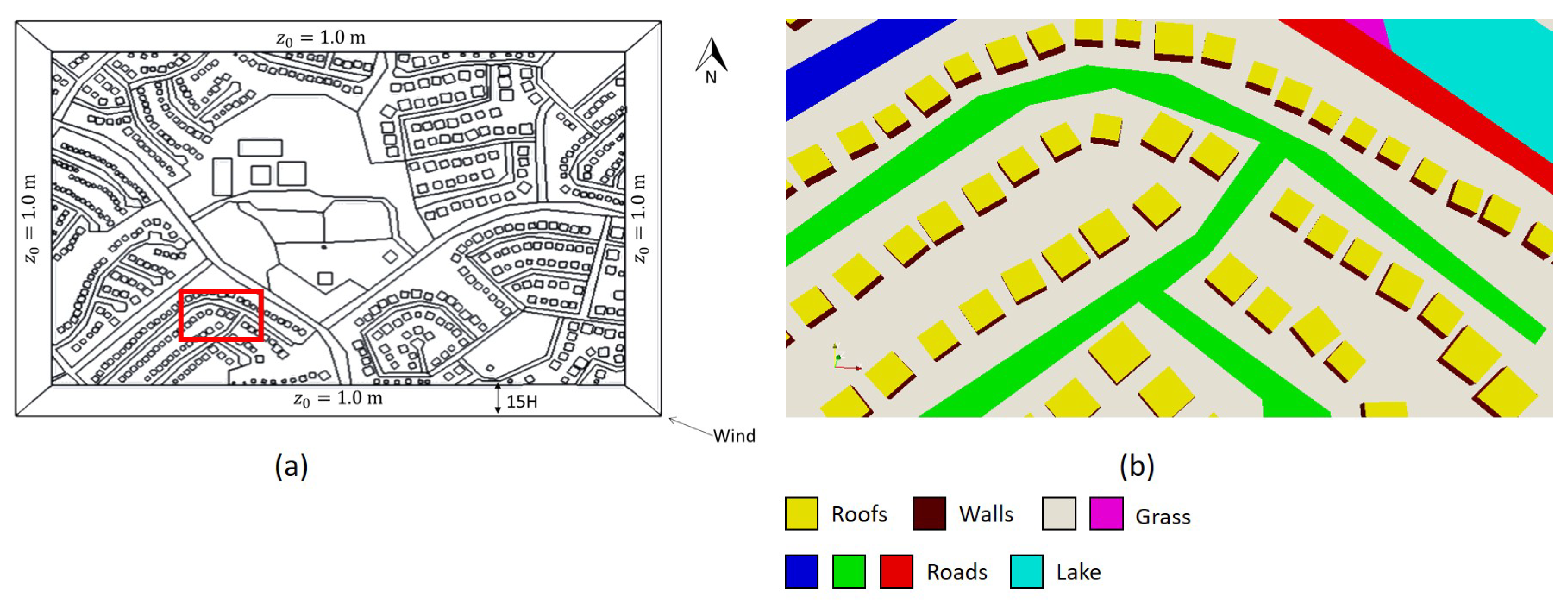
As a first step, the Power Ranch area was converted into an at-scale digital geometric model, as shown in
Figure 5a, with a close-up image of the buildings, road, and natural vegetation in
Figure 5b. As most of the buildings in the area were single-family homes, the height of all buildings was assumed to be
m. Following best-practice guidelines for urban CFD [
82], an additional boundary of width 15 H (75 m), perpendicular to the outer limits of the study area, was added. In the outer extent boundary, buildings were not explicitly modeled, but a aerodynamic roughness length
m was added, representing more suburban land-use with regularly-spaced buildings [
83], which corresponds to the land cover around the study area, as can be seen in
Figure 1b. The aerodynamic roughness length is the height at which the mean wind speed becomes zero, and is used to model land cover without explicitly resolving features such as buildings and trees. The top of the model was extended to a height of 15 H (75 m) above the top of the buildings. Small-scale objects, primarily trees and shrubs, were not directly modeled and, instead, the natural surfaces were modeled with a aerodynamic roughness length of 0.10 m, representing a roughly open terrain with a few trees and low hedges. Similarly, features on buildings (like windows or doors) and curb-side features in the residential areas were also not modeled. This was done to reduce the computational requirements to solve the equations.
For boundary conditions, meteorological data from the nearby Phoenix-Mesa Gateway Airport (measured at 1.5 m), together with surface temperature measurements from the mobile platform, were used, as shown in
Table 3. The far-field wind speed at the time of analysis was 0.45 m/s (about 1 mph) at a height of 1.5 m from an East-Southeast (ESE) direction. Using this value, an Atmospheric Boundary Layer (ABL) wind profile was applied at the boundaries, using the same aerodynamic roughness length
m, based on the recommendations of Raupack et al. [
84].
The far-field air temperature, as measured at the airport, was 42.22
C, and this was modeled as a uniform profile at the boundaries. The surface temperature of natural and artificial surfaces was based on the average values measured by the mobile platform: 50.36
C for roads, 48.19
C for natural surfaces, and 48.62
C for walls. As the platform could not measure roof temperatures, it was assumed that the roof was at the same temperature as the walls. This is most likely an underestimation of the roof temperature, as Stefanov et al. [
85] showed that roof temperatures in this area could rise to well over 70
C. However, in the absence of measured values corresponding to the hour at which this study was performed, this assumption was used. Furthermore, as the platform could not measure surface temperatures over water, it was assumed that the lake had the same surface temperature as the far-field air temperature. This was, again, possibly an overestimation, as the water would be significantly cooler than the air, but was used in the absence of measured data. It is possible that the effects of these over- and under-estimations would cancel each other out, to some extent, which will be verified during model validation.
4.3. Grid Convergence
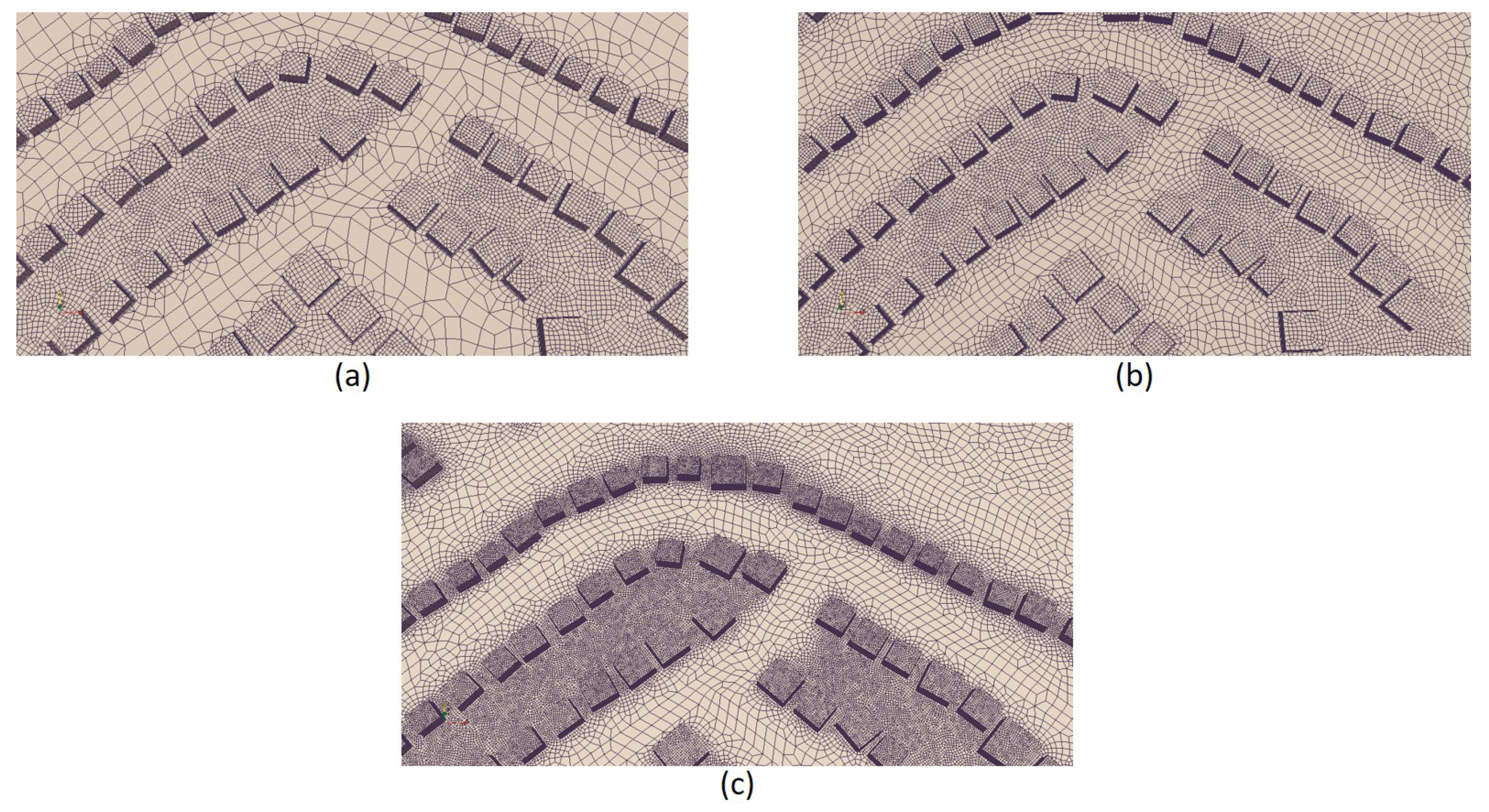
The digital model of the study area shown in
Figure 5 was discretized using the mesh extrusion method developed by van Hooff and Blocken [
86]. The 2D plan of the model (excluding buildings) was first discretized into quadrilateral elements of sizes varying from 1–5 m, and then the 2D mesh was extruded up to the height of the buildings. Next, the roof surfaces were discretized and the entire model was further extruded up to the top of the model. In this way, a high-quality hexahedral mesh could be generated. As a final step, boundary layer elements were added near walls, which were much smaller than 1 m. The meshing was done using the open-source meshing engine, Gmsh [
87]. All meshes generated consisted of over 99.9% hexahedral elements, less than 0.1% prismatic elements, and no tetrahedral elements.
A grid convergence study was performed to ensure that the results from the model did not depend on the size of the mesh. Three mesh cases were developed by approximately halving the size of cells from the preceding case. These are shown in
Table 4, with images from one part of the study area shown in
Figure 6.
For each of these mesh cases, the model was run until scaled residuals fell below ; except for pressure, where the final residuals were below . Lift and drag coefficients on the walls (which were functions of the wind velocity fields) were also monitored and, at convergence, they changed by less than 0.1% between iterations. The variables of interest in this study were the average wind speed and air temperature at a 2 m height over the two collector roads, given that most of the data was collected over the streets. These two variables were extracted from the model output.
To test for grid convergence, the difference between the average wind speed and air temperature over the roads at a 2 m height between the meshes was evaluated. For the Medium mesh, the difference was evaluated against the results obtained from the Coarse mesh, while, for the Fine mesh, the result from the Medium mesh was used. In addition to the difference, the Grid Convergence Index (GCI) recommended by Roache [
88] was also calculated using Equation (
4), where
is the difference between the average wind speed or air temperature at 2 m height,
is the refinement ratio for an unstructured mesh (the ratio between the number of cells in the fine grid
to the coarse grid
raised to the inverse of the number of dimensions), and
p is the order of convergence of the numerical scheme (second-order in this case,
). The GCI scales the difference between the variables of interest to account for grid refinement and order of convergence, providing a uniform way of reporting grid convergence studies. Both the differences and GCI for the mesh cases are shown in
Table 5.
For both the Medium and Fine meshes, the differences were small, with a maximum difference of 1.33% between the average wind speed over the roads. Similarly, the GCI values were also small, with the highest value being 7.77% between Medium and Coarse. Considering the inherent uncertainty in turbulence modeling and the unstructured nature of the mesh, these differences are acceptable. Thus, both the Medium and the Fine mesh cases were convergent within acceptable tolerance. However, as the Medium case was computationally faster, it was adopted for the remainder of the study.
4.4. Validation
Wind speed and air temperature over the road obtained from the Medium mesh case, as described above, were compared to the values measured during the hour of analysis by the mobile platform. As the platform moved along the transect, the points along which the measurements were taken changed continuously. Data obtained from between 5:00 p.m. and 6:00 p.m. was extracted and cleaned, yielding about 1000 points each for 2 m air temperature and wind speed. Points along the transect may not coincide with the center of a 3D element and, therefore, a point-to-point comparison of the two was not possible. This was in contrast to studies that used fixed weather stations for model validation. In this study, data from the computational model over the two main collector streets was extracted, yielding about 2000 points of data for each of the cases. The statistics of these two sets of data (measured and model) were, then, compared for validation. This approach is also logically valid, as the effects of the UHI (e.g., thermal comfort or energy use) depends on the value of air temperature within a localized region, and not the value at any single point.
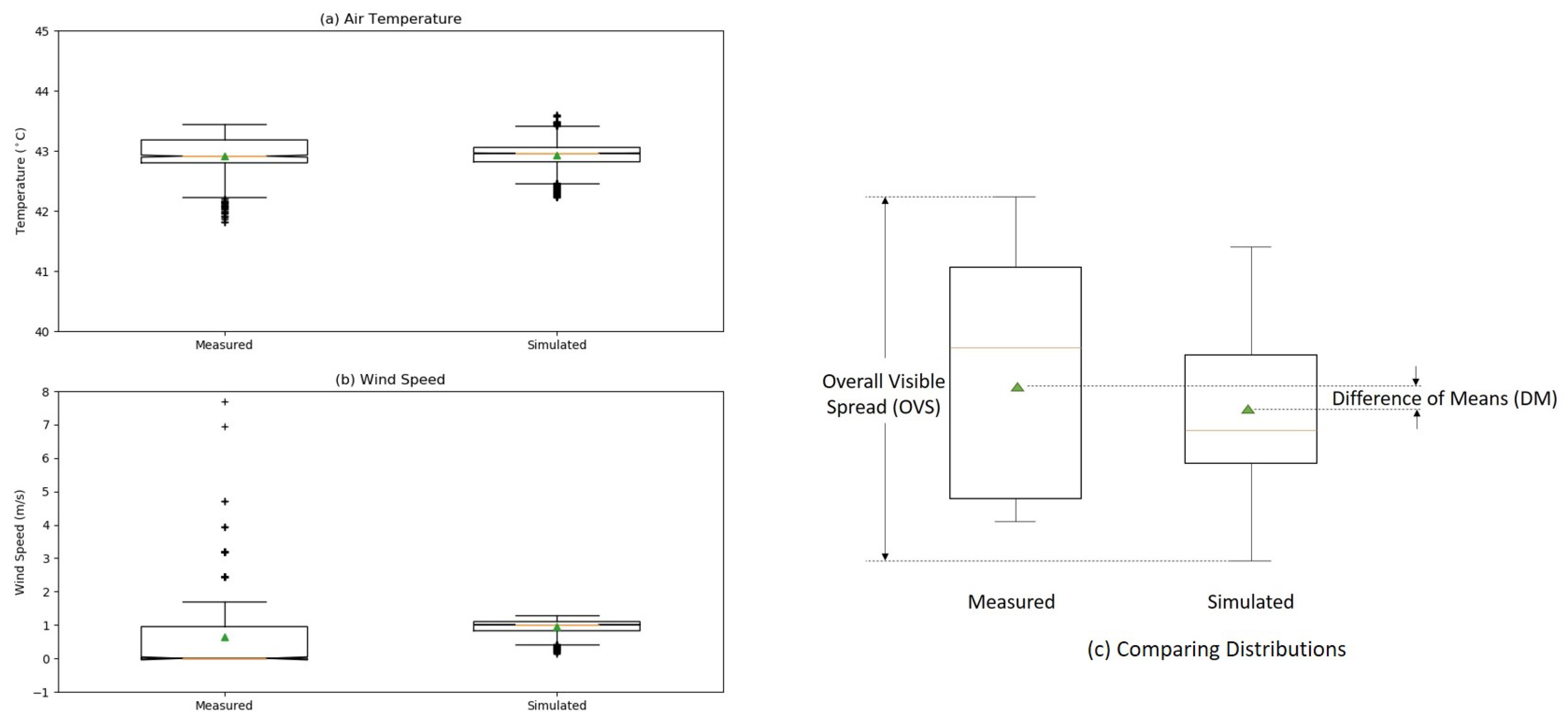
The results of the statistical comparison are shown in
Figure 7a,b, in the form of box-plots. It can be seen that the measured values, especially the wind speed, were highly skewed, with a large difference between the mean and the median as well as a number of outliers. Therefore, the validation must take both the mean and the distribution of the variables into account.
Two metrics were used, as shown in
Figure 7c. The Difference of Means (DM) is the difference between the mean of the measured and simulated variables. The Overall Visible Spread (OVS) was the overall range of the combined measured and simulated data, which is a measure of its distribution. An effective Coefficient of Variance COV
= DM/OVS was defined as a measure of variation between the measured and simulated data for each variable.
The DM for 2 m air temperature was just 0.03
C, while that between wind speeds was 0.47 m/s. The corresponding COV
were 3.0% and 28.0%, respectively. From these metrics, it can be concluded that the simulation showed excellent agreement with measured 2 m air temperatures, but only moderate agreement with wind speed. The difference in wind speed can be explained by the presence of a number of small-scale structures in the physical domain—such as trees, shrubs, and other vehicles—which decreased the local wind speed, but which were not explicitly modeled in the computational domain. As the mobile platform drove past these structures, it recorded a wind speed of zero or a low value below 1 m/s and, hence, over 50% of the recorded data was zero, as can be seen in
Figure 7b, where the median of the measured data is zero. Whereas, in the computational domain, they were not explicitly modeled and, thus, a higher wind speed was recorded at the corresponding locations, which, in turn, pushed the entire distribution to a higher mean value.
As the primary aim of this study was to examine the 2 m air temperature, the high degree of agreement between the measured and simulated temperatures and moderate agreement between the wind speeds were considered satisfactory for validation. This validated model was used to study UHI mitigation strategies.
6. Conclusions
The Urban Heat Island (UHI) effect is a commonly-observed phenomenon caused by increasing urban sprawl. UHI manifests in the form of increased urban air temperatures, and influences water use, air quality, public health, and so on. Cool surfaces, including pavements, roofs, and walls, have been suggested to mitigate UHI. However, the UHI is a heterogeneous effect, with local land-use patterns, construction materials, building forms, and climatic factors affecting possible mitigation strategies.
The microclimate of Power Ranch, a suburban development in the Phoenix Metropolitan Area, was studied for conditions at 5:00 p.m. on 13 August 2015, when the far-field air temperature was measured at over 42 C with a low wind speed of 0.45 m/ at a 1.5 m height from an ESE direction. An uncoupled pavement-urban canyon CFD model was developed and validated for the Power Ranch area. The area had two collector streets and several local streets, all of which consisted of aged asphalt pavements. Artificial surfaces (pavements, roofs, and walls) covered about 35% of the area, with the remaining 65% being covered by natural surfaces (grass, trees, soil, and water bodies).
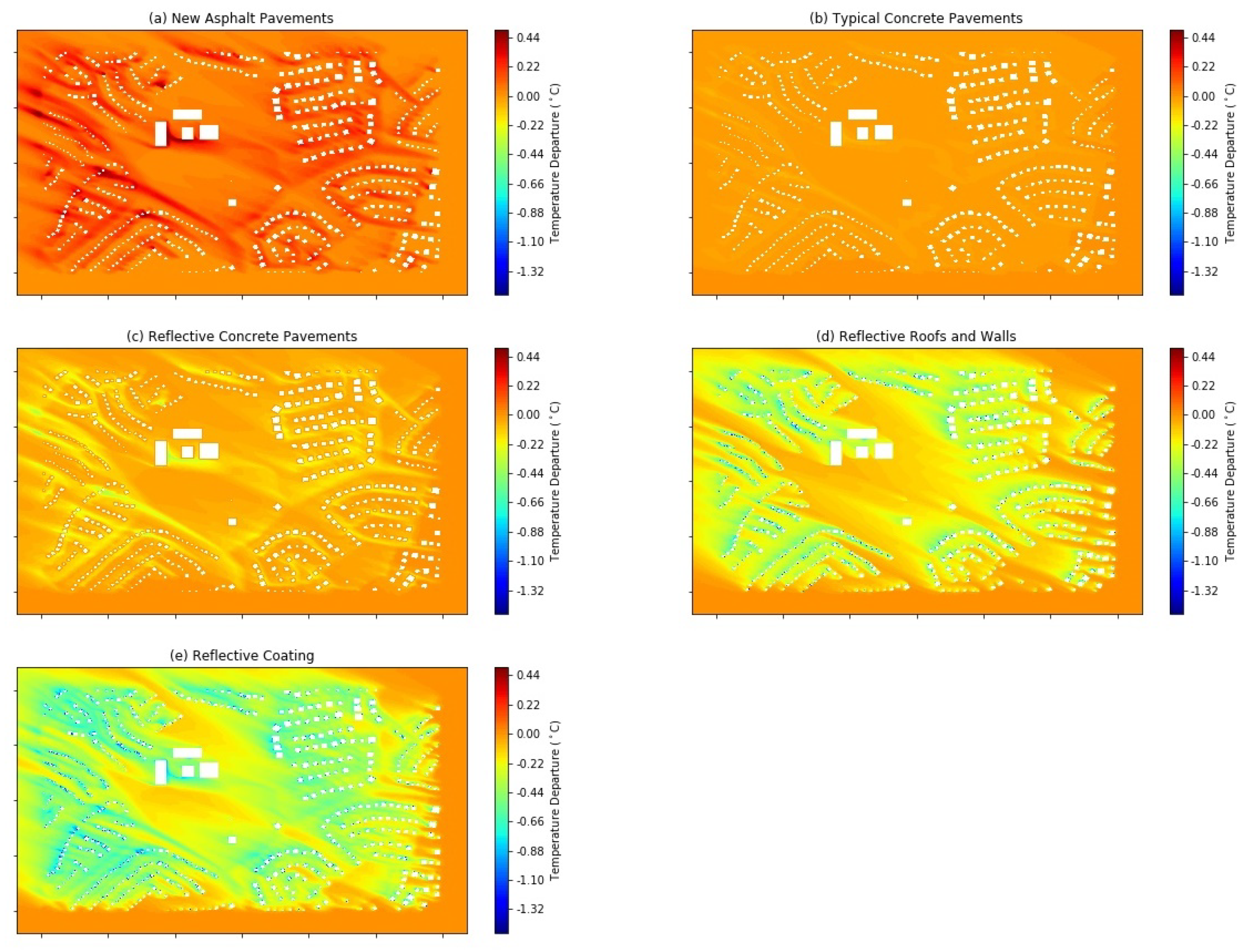
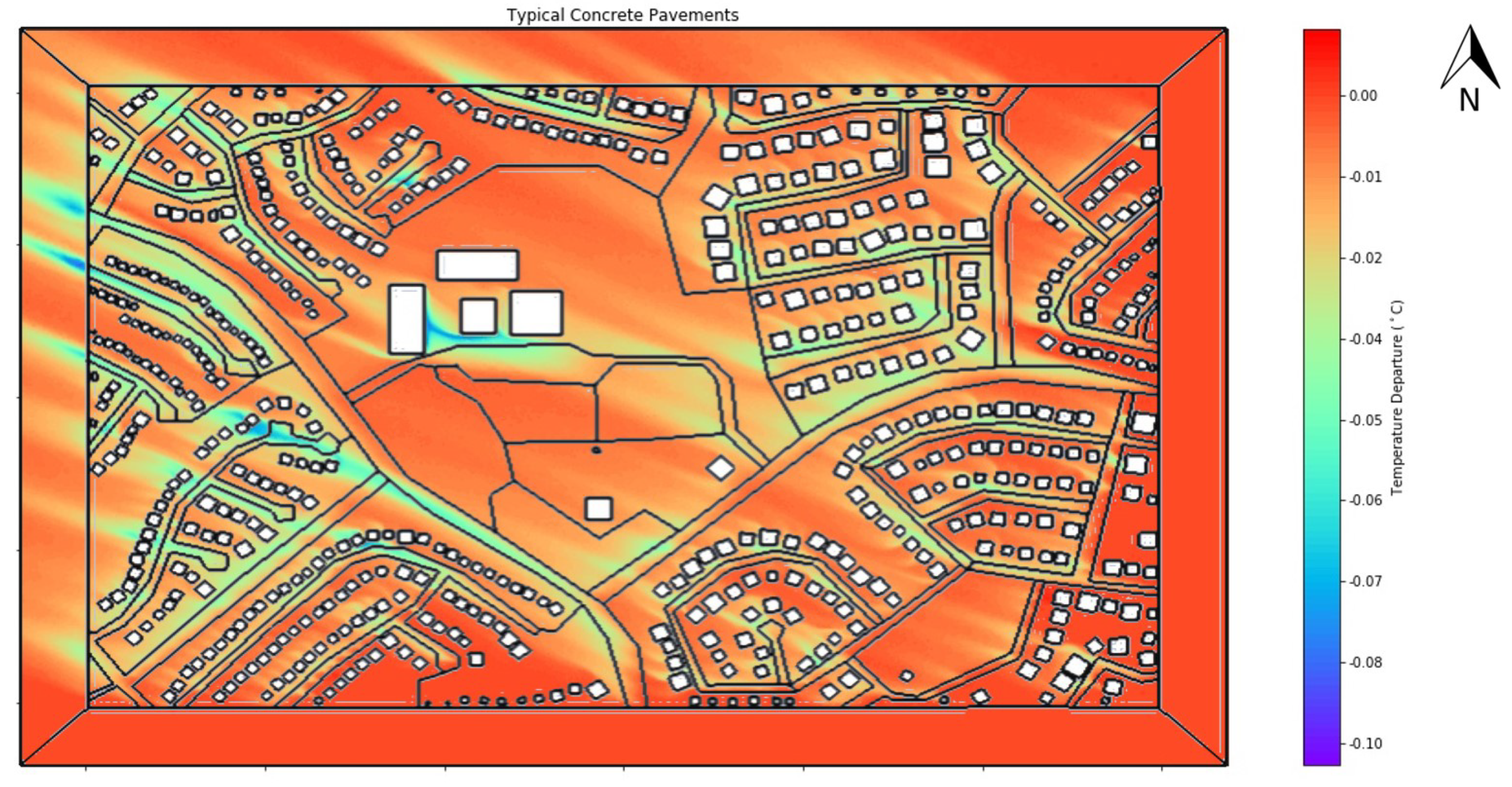
The effects of changing the pavement surfaces was investigated through five scenarios. In the first scenario, all aged asphalt surfaces were replaced with new asphalt surfaces. This led to an overall increase in air temperature at a 2 m height, with the maximum increase of 0.50 C being observed in the northwestern parts of the area; which were downstream of the collector roads. In the second scenario, the existing aged asphalt pavements were replaced with typical concrete pavements. This strategy, for this neighborhood, led only to a slightly decreased air temperature of less than 0.1 C, with the large area of the natural surfaces largely negating the decrease in temperature from the cooler pavements.
The third scenario replaced all pavement surfaces with more reflective concrete pavements. This led to a decrease in air temperature by about 0.20–0.40 C downstream of the collector roads. However, there was no significant reduction over most of the natural surfaces. A fourth scenario coated all roofs and walls with a reflective coating, leading to a higher 2 m air temperature reduction, of about 0.40–0.70 C, and a small decrease, of 0.00–0.10 C, over the natural surfaces. Finally, a fifth scenario increased the albedo of all artificial surfaces with the same reflective coating. This scenario resulted in the largest decrease in air temperature, by about 0.80–1.00 C, in the northwestern development downstream of the collector roads, as well as a decrease of 0.10–0.20 C over the natural surfaces.
Thus, for the meteorological conditions evaluated for the Power Ranch suburban community, changing all walls, roofs, and pavements into reflective surfaces was the most effective strategy for mitigating UHI. Using only reflective walls and roofs had a greater mitigating impact than using only reflective pavements. For existing suburban developments, applying reflective pavements is likely to be implemented faster, whereas reflective roofs and walls would require the participation of a large number of homeowners. These conclusions are only for the particular land cover type, analysis period, and meteorological conditions of this study. A similar type of study would need to be conducted for the unique conditions of other locations for the mitigation of UHI.


