The Impacts of Economic, Demographic, and Weather Factors on the Exit of Beginning Farmers in the United States

1
Department of Agricultural Economics and Rural Sciology, Auburn University, Auburn, AL 36949, USA
2
Consumer Product Safety Commission, Bethesda, MD 20814, USA
*
Author to whom correspondence should be addressed.
Sustainability 2019, 11(16), 4280; https://doi.org/10.3390/su11164280
Submission received: 1 June 2019
/
Revised: 25 July 2019
/
Accepted: 31 July 2019
/
Published: 8 August 2019
(This article belongs to the Special Issue Agricultural Production and Global Climate Change: Social, Cultural, and Agroecological Aspects of the Agriculture/Climate Interface)
Abstract
:The success of efforts to promote sustainability and growth of Beginning Farmers and Ranchers (BFRs) depends on a set of diverse factors whose individual impacts on the BFR survival in or exit from farming need further clarification. This paper evaluates how a variety of economic and demographic factors, together with weather variability, affect BFRs’ exit from farming using farm-level data from the US Census of Agriculture for the period 1992–2012. The analysis uses insights from the literature on firm exit, recent research on young and beginning farmers, and the literature on climate impacts on agriculture since weather remains a key input to farming and its variability is a major source of risk to less experienced BFRs. The main finding is that flow variables such as profitability and off-farm employment do not affect BFR exit, while reliance on government payments increases the exit probability. Consistent with previous work, the size of operations matters, as BFRs with larger asset ownership, higher sales, and those in livestock production have lower probability of exit. Price variability that affects exit is largely attributable to weather variability, a finding which is consistent with that of previous work. The weather impacts on BFR exit are mostly attributable to droughts, but temperature also has a non-linear and highly seasonal impact.
1. Introduction
Beginning Farmers and Ranchers (BFRs) are farmers and ranchers who have been operating a farm for 10 years or less. This group accounts for 22% of all US farms and 10% of the total value of production [1]; 20 percent of family farms were classified as beginning farms in 2015 [2]. At the same time, the latest quinquennial Census of Agriculture shows that, over the last decade, the number of BFRs has decreased by about 21%. Yet, recent research shows that the actual number of new farm entrants may be as much as double the previous estimates [3]. These contradictory findings point to the need to understand better what drives BFR success and identify the factors that contribute to their survival in order to ensure sustainability of US agriculture.
In the past few decades, there have been numerous efforts to evaluate the needs of new farmers and offer educational, financial, and other support programs to ensure their survival and success. For example, several programs such as the Aggie Bond program established in the 1980s and the support programs through the 1992 Agricultural Credit Improvement Act were developed to provide beginning farmers access to capital [4]. The most recent Agricultural Act of 2014 also contains provisions for crop insurance programs, Farm Service Agency loan programs, and the Conservation Reserve Program’s Transition Incentive Program [5]. However, it is unclear if such programs are sufficient to ensure BFR ability to remain in farming, since the factors that affect BFRs success or exit need to be better identified.
The analysis presented in this paper utilizes an empirical framework grounded in a theoretical model of intertemporal utility maximization to evaluate what factors affect BFR exit. The analysis uses insights from the firm entry and exit literature and the literature on young and beginning farmers and is also influenced by the growing literature on climate impacts on agriculture, since weather remains a key input in farming and its variability is a major source of shock to more vulnerable BFRs. To gain longer-term insight, we use 20 years of data from the US Census of Agriculture for the period 1992–2012 and evaluate how the weather variability, part of which could be attributed to climate change, together with a variety of economic and demographic factors, affect BFRs’ exit from farming. To date, we are unaware of work that has incorporated how weather affects success and exit of BFRs.
Weather variability is likely to affect BFRs’ exit because new farmers are less experienced, have fewer resources, and less time perspective to make costly adaptations to variation in weather patterns. To mitigate the impact of weather, farmers must change profit maximizing crop mix [6] or adopt new crop varieties resistant to weather extremes [7]. This is not easily achievable by new farm operators. Moreover, there is evidence of high sensitivity of the US crop yields to extreme heat, in spite of the introduction of new genetic traits and improvements in infrastructure [8]. Even measurable improvements in heat tolerance for various crops are found to come at the cost of average yield reductions, which affect farmers’ profits and thus the likelihood of exit [9]. At the same time, there are also estimates showing a 4% increase in annual profits resulting from climate change, suggesting that farmers’ wellbeing is affected directly by the weather variability attributed to climate change [10].
This paper addresses certain gaps in the farm exit literature, which is largely fragmented and a little dated. For example, for an earlier period between 1978 and 1997, Hoppe and Korb [11] found that larger farms are less likely to exit, suggesting that smaller BFRs are more vulnerable. In addition, there are few nationally representative studies, and studies are typically focused on individual commodities (i.e., dairy) [12], or farmers overseas [13,14], which are less useful for policy purposes. Recently, Katchova and Ahearn [3] computed exit rates for farmers from various age cohorts but did not study what factors affect exit, and Williamson [15] showed significant age-related difference the in growth trajectories of surviving BFRs between 1999 and 2014.
The main objective of this paper is to identify the factors that affect BFR exit. The factors are grouped into cash flow related variables (return on assets, sales, price variability, and government payments), stock variables (assets), demographic and industry type variables, and variables measuring the impact of climate variability. This research contributes to the literature on farm survival and sustainability of the agricultural sector by expanding the range of explanatory variables using detailed farm level panel data spanning 20 years at the turn of the century. Our results indicate that price variability that affects exit is attributable to weather variability, which is consistent with previous work. The strongest impact of weather on BFR exit is attributable to droughts, but temperature also has a non-linear and highly seasonal impact. We also find that, while flow variables such as profitability and off-farm employment do not affect BFR exit, reliance on government payments increases the probability of exit. The size of operations matters as BFRs with larger asset ownership, higher sales, and raising livestock have lower probability of exit.
The rest of the paper is organized as follows. The next section contains a review of the relevant literature. Section 3 presents the empirical approach. Section 4 describes the Census of Agriculture data on BFRs and the divisional climate variation data. Results are discussed in Section 5. The final section offers conclusions.
2. Review of the Relevant Literature
This work lies at the intersection of several areas of the existing literature. It is related to the literature on young and beginning farmers, the literature on farm entry and exit, and the literature on climate impacts on agriculture.
Most of the relevant literature on young and beginning farmers is concerned with identifying how BFRs may be different from established farmers, what their specific challenges are, constraints and growth opportunities, and what affects their growth and, to a lesser extent, survival. The general conclusion of this literature is that the BFRs are obviously younger, more educated, include a higher percentage of women and minorities, have smaller size operations and limited access to loans, own less land and assets, and are not a homogenous group in terms of growth opportunities. In terms of age, evidence shows that nearly one-third of BFRs were aged younger than 50 [16]. In terms of asset ownership, Mishra et al. [17] found that established farmers had roughly twice the amount of assets as BFRs, which largely reflects the difference in land tenure. Ahearn [1] observed that BFRs are more likely to lease land than established farmers, as well as purchase land from non-relatives while Hartarska and Nadolnyak [18] showed that 54% of BFRs purchased land from non-relatives, which is related to BFRs various performance indicators such as higher debt-to-asset and asset turnover ratios.
Since agriculture has high capital requirements and lenders have stringent lending standards, young and beginning farmers may face difficulties in accessing loans to buy land due to restricted access to credit [18,19]. Their growth prospects are also very diverse with younger farmers having better opportunities even though they are less likely to own and more likely to rend land [5,15]. This has an interesting implication: since BFRs own less land, they are less exposed to fluctuations in land values because rents are relatively sticky. Thus, BFR repayment capacity is less affected by economic downturns than that of established farmers, although the BFRs still are more vulnerable to shocks [4].
There have been many government programs targeting BFRs, many related to access to capital, with differential success [4]. Relevant to our work is the result that government support policies have differential impacts on BFRs and on established farmers. For example, Kropp and Katchova [20] find that government direct payments are positively and significantly related to experienced farmers’ term debt coverage ratio, while government payments had no effect on the BFRs debt coverage ratios.
Recent exit rates estimates for young and beginning farmers and ranchers were estimated in the work of Katchova and Ahearn [3], who used census data. Their exit rate estimates are comparable to the present study but the objective of that study was not to show how economic and demographic factors and climate variability affect farm entry and exit. Our work not only fills this gap but is also related to the farm exit in the entire farming population and not only for the BFRs. Outside the field of agricultural economics, research in social sciences explores how farmer demographics, social constructs, family circumstances (i.e., successor identity), and social attributes (i.e., early childhood socialization) affect farm exit [21,22].
Early work on farm succession is less relevant because it was focused primarily on the impacts of tax considerations on farm exit decisions [23,24,25]. More relevant work related to farm succession is focused on how the new and mostly commercial farmers overcome borrowing constraints [26]. Somewhat relevant is the literature on succession that evaluates the role of farmer demographic characteristics, asset allocation, support payments, and off-farm work. There is evidence that the choice of successor is affected by farm operator education, age, off-farm employment, expected household wealth, geographic location, and government policies [27]. In terms of general farm exit, there is also evidence that higher direct government payments had a small but statistically significant negative effect on farm failure that increases with farm size [28]. Larger debt to asset ratio has also been associated with a higher exit rate. Similar work finds negative association between decoupling government payments and the overall exit rates but positive association between decoupling and disinvestment in land and machines, which suggests that policies affect rescaling of production and can facilitate exit of failing or aging farmers [17,29,30].
Other work that uses county-level census data finds no association between government supports and off-farm employment and farm exit but a positive association between grouping counties by the net change in the number of farmers [31]. There is also evidence of negative association between capital accumulation and off-farm work, as well as evidence that off-farm employment is affected by the volume of farm output and producer demographics [32,33].
Our work is also related to that of Gutter and Saleem [34] on US farm financial vulnerability, that studied farm retirement decisions and highlighted the impacts of idiosyncratic risks such as weather or commodity price fluctuations on farmers’ short-term finances. So far, the growing literature on the impact of climate variability and weather on agriculture has not incorporated weather risks either in general farm or in BFRs exit in the context of how systematic weather fluctuations affect farmer financial positions, profitability, and exit.
We believe there are several reasons why this topic is under-explored. There is evidence that the US crop yields continue to be highly sensitive to extreme heat in spite of new genetic trait development and infrastructure improvements [8]. Moreover, in the past 40 years, there has been little evidence of adaptation to climate variability by the US producers, possibly due to lack of incentives [35]. Some research attributes the lack of association between weather and farm incomes to the opposite impacts of the weather on output and prices [36]. Other researchers have found that, while dairy production was negatively correlated with local average temperatures, there is no relationship between temperature deviations and dairy production [37]. One of the reasons for this observation might be that farmers work more hours when the weather is bad in order to compensate for the lower productivity. Indeed, Lee et al. [38] found a nonlinear relationship between farm labor and temperature and a linear negative impact of precipitation.
Another reason why the possible impact of weather variability as an idiosyncratic risk on farmers’ incomes and exit is not fully explored is the existing belief that financial markets and supporting infrastructure effectively negate the impact of weather variability. However, there is evidence that highly leveraged farmers are affected by negative weather shocks which is reflected in increased delinquency rates of agricultural real estate loans by the Farm Credit System (FCS) and by commercial banks, but the overall financial performance of these lenders remains unaffected [39].
3. Methodology
The theoretical underpinnings of the empirical model lie in constrained inter-temporal utility maximization the reduced form of which is a value function of not exiting [14,29,40]. The present value of the utility of consumption and leisure is
where Cτ and Lτ are consumption and leisure at τ, and is the τ to t discount factor. The intertemporal budget constraint is
where is the net asset value at t, wτ is off-farm wages, per period time endowment is 1, Fτ is gross income from farming, and rτ|t is market discount rate as opposed to the discount factor . Assuming irreversibility of the exit decision, the value of exiting is in (1) maximized with respect to (2) when Fτ = 0 which is a function of the variables that affect on-/off-farm utility and income such as farmer attributes and local economic and institutional factors. The present value of not exiting at t is
It is worth noting that this setup can accommodate disinvestment or downscaling (sale of assets) that may be optimal exit. , the difference between the values of staying and exiting, can be called the tendency to exit that increases with variables that positively impact current off-farm utility and decreases with variables that positively impact current on-farm and future off-farm utility, which accommodates both direct and indirect impacts of the variables, i.e., changes in off-farm labor markets affecting both current and future off-farm utility, age and education affecting the utility of staying and exiting, and farm income increasing the on-farm utility but also leading to changes in labor-leisure allocation that might encourage exit. The exit decision rule according to the tendency to exit defined above is an index function.
whose first-order estimable approximation is
where Xt is the vector of the variables that directly affect current and future on- and off-farm utility, including shifters such as personal and location-specific attributes and institutional factors. If the approximation error εi is assumed to be standard normal, the coefficients in can be estimated using the standard probit model with the cumulative in the log-likelihood function being standard normal over (−∞, βXt). Consequently, the probability of observing exit and disinvestment is modeled as:
The variables in X are selected according to the relevant empirical findings and include on- and off-farm income and demographic variables, measures of profitability, agricultural subsidies, and macroeconomic and regional characteristics. Specifically, the empirical model includes farm-level return on assets (ROA), total assets (LnAssets), a family farm dummy (FAMILY), and a dummy for livestock type farm (LIVESTOCK). The controls include the government payments received (GPAYMNT) as an institutional factor, as well as the state-specific nonagricultural share of GDP (NONAGSHARE) and county-level unemployment rate (UNEMPRATE). The standard deviation of the output-input ratio in the period during which exit has occurred (PRICE_RISK) is used to control for the riskiness of farming. We also added regional and time differences by adding dummies for the census year of the observation (CYEAR) and dummy variables for the 10 agricultural production regions. The regions are: Southeast (SE), Appalachia (AP), Corn Belt (CB), Delta (DLT), Lake States (LS), Mountains (MTN), Northeast (NTE), Northern Plains (NP), Pacific (PAC), and Southern Plains (SP). See the data section for a description of all the variables.
The climate impact literature has shown that climate variability and weather may affect profits negatively and thus speed up exit. Thus, we include climate variables in the form of seasonal cumulative heating and cooling degree days (HDD and CDD) and standard deviation of the rainfall index.
Farmer demographic characteristics include dummies for age (AGE) and race (MINORITY). The variable definitions are listed in Table 3.
4. Data
The analysis uses the latest available farm-level Census of Agriculture panel data from surveys conducted in 1992, 1997, 2002, 2007, and 2012. The latest 2017 Census data is only about to be released for research purposes, a delay attributed to the recent government shutdown. Not all farmers participated in the long form survey of the Agricultural Census and the maximum number of records are constrained to 1992–2002 because only a subsample of farmers surveyed provided information on their assets size. For more on Ag Census Sampling see: http://agcensus.mannlib.cornell.edu/AgCensus/censusParts.do?year=2002. The dataset includes about 112,000 records or about 28,000 BFRs per census period. The rainfall and temperature estimates come from the National Oceanic and Atmospheric Administration (NOAA) and account for systemic risks stemming from climate variability. The rainfall index is defined as the first principal component (PC1) of standard deviation-normalized rainfall series. Employment information and wages were collected from the Bureau of Economic Analysis (BEA) and profitability for state and national inputs and outputs was published by the USDA’s economic Research Service (ERS). The ERS publishes state productivity figures, including inputs and output prices and standardized quantities, by input type and commodity sold. The indices are only available for from 1960 through 2004. The state GDP data are from the Bureau of Labor Statistics (BLS).
The panel is constructed by linking observations from Agricultural Census years to form a long panel using individual farm operator IDs. The sample only includes farmers that qualify as BFRs, namely observations for farmers where current Agricultural Census year minus the year when farming activity started is less or equal to 10 years. Individual observations only include beginning farmers earning at least 2000 USD in a given census year. The final census year to which a beginning farmer responds is coded as zero and as 1 if there is no observation in the following census year but the farmer would still be in the BFR category. The last available census year of 2012 is used to establish if a farmer qualified as being a BFR (less than 10 years of farming) in any previous year but was in the sample as non-BFRs in 2012. If he/she is in the sample, then these farmers are considered surviving (zero) while if there is no record, then that farmer is coded as exited. Thus, farmers who remained in farming and non BFR were not coded as exits but a zero.
Table 1 shows (the annualized) exit rates by region. The regions that we use are Southeast (SE), Appalachia (AP), Corn Belt (CB), Delta (DLT), Lake States (LS) Mountains (MTN), Northeast (NTE), Northern Plains (NP), Pacific (PAC), and Southern Plains (SP). All regions experienced a decrease in 5-year exit rates between 1992 and 2012. Our annual rates compare well to those of Katchova and Ahearn, who found exit rates of 9.1 for BFRS the period of 1997–2002, 9.0% for 2002–2007, and 7.6 for 2007–2012, while our estimates are slightly below that at 7.5, 7.8, and 9.8, respectively. The Lake States (LS) had the smallest exit rate on average, followed by the Corn Belt (CB) that had notable decrease in exit rates between 1992 and 2002. This suggests that, during this period, many BFRs remained in farming. All regions experienced sharp decreases in exit rates between 1992 and 1997, but this leveled off in 2002 and the period of 2007–2012 saw an increase in BFR exits. Since that period was generally good to agriculture, it could have been due to the fact that many non-beginning farmers remained in farming thus limiting the opportunities for those at the beginning of their farming careers.
Table 2 shows the ratios of farmers working off-farm to the number of farmers exiting. The variable WRKOFF is a dummy variable that equals one the BFR worked outside the farm and zero otherwise. The ratio is less than one for most regions and periods and with a peak in the 2002–2007 period, suggesting that working off-farm can either be a precursor to exit or a means of subsidizing farm activities.
Table 3 lists descriptions of the key explanatory variables. The gross return on assets (ROA) is defined as the gross income (computed by subtracting production expenses from the total value of production) divided by total assets (ASSETS). ASSETS are defined as the sum of the value of land, buildings, and machines. The natural log of the assets (lnASSETS) is used to account for scale. In addition, two sales class dummies are constructed: Midsales and Highsales, based on the total value of production (TVP), namely $100,000 < TVP ≤ $500,000 and TVP > $500,000 respectively.
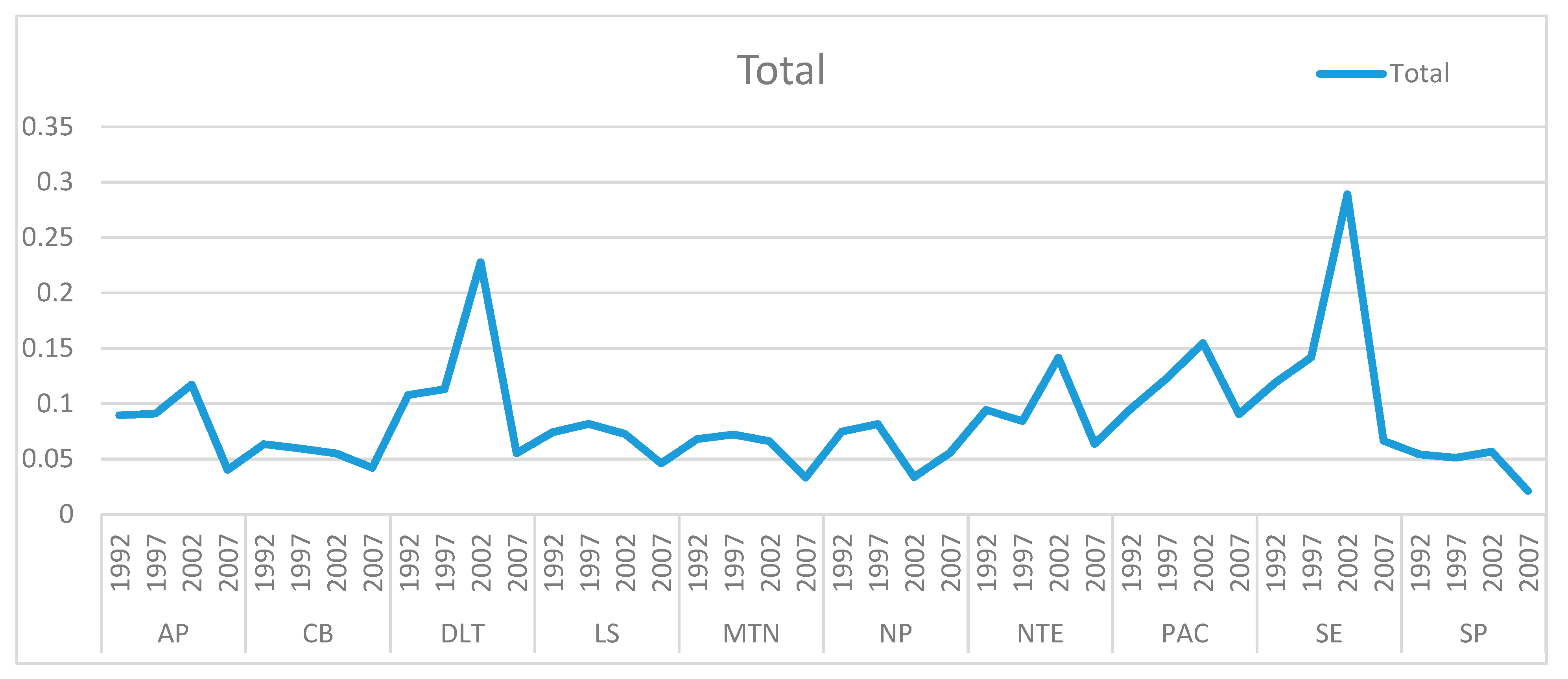
Table 4 shows the means of the key variables by census year (Census YEAR). The exit rates decrease over the 1992–2002 period, in contrast to the ROA that rose between 1997 and 2002, peaking at 0.146. Figure 1 plots ROA by region and Census Year. Most regional ROAs peak in the 2002–2007 period.
The Corn Belt and Northern Plains saw a decrease in ROA during this period and the Mountain states had a nearly flat ROA from 1992 to 2007. GPAYINT is the greatest in the period beginning 1992 at 0.19 and only 0.16 by 2007, indicating that government payments are growing less than revenues in real terms. The average farmer age increases over the series from 43.1 to 47.0 years of age so BFRs were aging as a whole. The percent of family farms by BFRs increases over the series from 82.5% to 84.1%. The percent of livestock enterprises decreased from 52.3% in 1992 to 46.0% in 2012. The proportion of BFRs with Mid Sales dropped from 13.8% to 11.5%, while that for High Sales rose 2.4% to 4.6%, respectively.
The proportion of BFRs within some regions changed while in others it was remarkably stable. For example, the percent of farmers classified as BFRs in Appalachia decreased from 13.9% to 10.9%, in the Corn Belt it fell from 20.9% to 18.3%, and it fell only slightly in the Delta from 5.5% to 5.2%. It fell from 9.5% to 8.9% in the Lake, and from 9.3% to 8.8% in the Northern Plains. During the same period, the percentage of BFRs in Mountains increased from 6.6% to 7.8%, and increased from 6.1% to 8.8% in the North East, from 8.2% to 9.4% in the Pacific, slightly increased from 6.8% to 7.1% in the Southeast, and increased from 13.2% to 15.7% in the Southern Plains. In terms of other demographic changes, we observe that the percentage of the non-white BFRs hovers between 0.1% and 2.2% showing that the BFR group is racially homogenous which could be either a function of the $2000 cut-off or the actual composition of BFR startups. The proportion of farmers working zero days off-farm varies over the series from 0.328 to 0.273, so overall there are more BFRs working off-farm.
The climate data are summarized in Table 5 and Table 6. Choosing the right measures of the impact of climate is always a challenge because various crops have different tolerance to temperature extremes. While the most popular measures are the temperature and precipitation or the El Niño-Southern Oscillation (ENSO) variation, in this paper, the focus is on variability over a period of time that may affect farmers’ decision to exit. Thus, we measure the impact of climate variability by the standard deviation (variability) of three indicators all averaged by season (spring, summer, fall and winter) for the five years period ending with the census year t + 5 (used to determine if a BFR would have exited or not).
In order to measure the impact of precipitation and capture the effect of droughts, we use the variation (standard deviation) in the rainfall index, adding SPRING_SP3, SUMMER_SP3, FALL_SP3, and WINTER_SP3. These variables are derived from the monthly Standardized Precipitation Index (SPI) collected from the National Oceanic and Atmospheric Administration (NOAA) database at the divisional level [8,10]. We were able to match US counties with divisions using the NOAA climate prediction center. It is important to note that not every county rests entirely in a single Division. To solve this problem we took the approach that if at least 10% of a county’s area appears to lie within more than one division, we assign it to the division where most of the area lies and then add a flag for multi division. In the case of close proportions, we randomly assign its divisional membership. http://www.cpc.ncep.noaa.gov/products/analysis_monitoring/regional_monitoring/CLIM_DIVS/states_counties_climate-divisions.shtml. SP3 is the variance of the SPI index aggregated by 3-month seasons. SP3 = 0 reflects the median of the distribution of precipitation, a value of −3 indicates a very extreme dry spell, and +3 indicates a very extreme wet spell. Degree days represent the absolute difference between 65 °F and the average temperature (daily high–daily low)/2. Days with a temperature higher than 65 °F are called cooling days, and days with a temperature lower than 65 °F are called cooling days, on account of the need to heat (cool) the home, respectively (National Weather Service, URL: http://www.srh.noaa.gov/key/?n=climate_heat_cool). We use the NOAA Climate division three-month precipitation index (SP3) to control for rainfall’s effect on profitability expectation and exit.
Table 5 summarizes the standard deviations of rainfall variation based on the previous five values. We observe that, during the study period, rainfall variability in spring and summer moves in the same direction with lowest variability in the middle of the period around 2002, while larger variability is shown for the beginning and the end of the study period. This is the opposite to the rainfall variability in fall which has the highest variability in 2002 and the lowest variability at beginning and the end of the study period. The lowest variability is observed in the winter months.
We use the total cooling and heating degree days to capture the impact of temperature, i.e., Total Heating Degree Days variability (Season_HDD) and seasonal Total Cooling Degrees Days variability (Season_CDD). Degree days are defined as the number of degrees by which the average daily temperature is higher than 65 °F (cooling degree days) or lower than 65 °F (heating degree days). For example, one day with an average temperature of 90 °F equals 25 cooling degree days—the same as 25 days with an average temperature of 66 °F. It measures the extremes in and duration of high and low temperatures that are detrimental to agriculture. The original means, standard deviations, and variances were calculated for each season over the five years ending with the census year. The climate summary statistics presented here are the means of the 5-year original statistics by county, thus are the original divisional statistics weighted by the number of counties in a given division. These variables capture both how much (by what degree) and for how long (how many hours and days) the temperature is above 65 °F (cooling degree days) or below 65 °F (heating degree days). Therefore, they represent a good approximation to the exposure to extreme temperatures by plants and animals as opposed to average annual temperate or its extremes that are less informative for how long each heating of cooling spell.
We use both CDD and HDD instead of GDD for two reasons. One is that, looking for weather impacts on profitability, it is necessary to account for the damages from extreme heat and that is why we include the CDD as well. Second, GDD is crop-specific and the base temperature ranges from 35 °F for onion to 60 °F for sweet potato and eggplant, which makes GDD less relevant and precise for analyzing farm financial performance without knowing what the farm is growing.
5. Empirical Results and Discussion
Table 7 presents results from the two specifications: one with all the variables except those measuring climate variability and one with the climate variables. Another difference between the two specifications is that the first column also includes a price risk measure computed as the five-year standard deviation of the output-input price index that generally captures price variability. This variability is also computed in the same way as the climate variables from period t to period t + 5, since exit happens during that period of time. This variable is strongly correlated with the climate variability measures and with the Census Year dummy and cannot be included in the second specification to avoid multi-collinearity. In fact, this coefficient is automatically dropped by the software. The high level of correlation indicates that our choice of the climate variability measure is probably a good approximation since it is likely affecting the price variability captured by the standard deviation in the input-output price index. We avoid the impact of outliers by excluding the top 99th percentile or higher income and the bottom 1. Acres are averaged 247 over the five census periods. Interpretation of the probit coefficients is cumbersome due to the nonlinear nature of the model and, since the coefficients are only valid for small deviations from the variables’ means (since the model itself is non-linear), we present the marginal effects in a column next to the coefficient estimates.
The main objective of this paper is to identify the factors that affect BFR exit and we have grouped these into cash flow related variables (ROA, sales, price variability, and government payments), stock variables (assets), demographic and industry type variables, and variables measuring the impact of climate variability. The results indicate that the main cash flow variable, ROA, does not affect the BFR exit. This was true for all but one alternative specification that we estimated and in the one where ROA was significant it was positive and significant at the 10 percent level. However, government payment intensity (GPAYINT) is significant and positive with the marginal impact of a one percent increase in the share of government payments on the probability of exit in the following census interval being 1.7%. This result is somewhat different from that of Key and Roberts [28] who found that government payments decreased county-level exit, but in line with that of Kazukauskas [30] who showed that reliance on government subsidies increases disinvestment. However, neither of these studies examined BFRs separately. Other work has shown that government policies affect BFRs and experienced farmers differently. For example, Kropp and Katchova [20] found that, while direct payments were positively related to financial variables of experienced farmers, they had no effect on those of beginning farmers.
Another variable capturing the impact of current income is the WRKOFF dummy, which is not statistically significant, showing that access to additional employment has no effect on BFRs’ decision to continue farming suggesting that off-farm work is likely used to supplement farming or consumption and not as a clear substitute to farming. The results on the flow variables are almost exactly the same in the two model specifications.
Given the distribution of government payments toward more established farmers with historical program acreage, other factors such as asset ownership and cash rents on program acres would provide useful insight. Indeed, the variables capturing economies of size and asset ownership are statistically significant predictors of exit. Specifically, we find that LnASSETS is significant and positive across all specifications indicating that one percent increase in LnASSETS is associated with 0.017 lower probability of exit. Thus, we find that asset ownership is among our main predictors for remaining in farming among BFRs and, considering that Ahearn and Newton [16] find that beginning farmers face higher startup costs and lack access to land (to purchase or rent) relative to established farmers, policies to encourage ownership seem appropriate. Furthermore, our result is consistent with that of Katchova and Ahearn [3] who found a stark contrast within the BFR group with younger farmers showing a higher growth trajectory measured by operated acres (also more likely to rent their land), which decreases the likelihood of exit. Kauffman [19] argues that the higher capital requirements and stringent lending standards may limit BFRs’ ability to own land due to restricted access to credit. BFRs with land ownership are more likely to gain access to loans, expand operations, and take advantage of economies of scale and favorable market conditions. The negative link between asset ownership and exit suggests that various government programs targeting BFRs with special loans and guarantees remain pertinent for the success of BFRs [4].
We also found that BFRs in livestock production are slightly less likely to exit relative to those in crop production (marginal effect is −0.011), possibly due to larger exit barriers due to asset specificity and vertical integration in many of the livestock industries. The marginal effects for farm sales classes show that, relative to the BFRs with less than $100,000 in sales, BFRs with sales classified as MIDSALES are 2% less likely and those classified as HIGHSALES are 5.3% less likely to exit farming by the following Census Year. The two specifications produce exactly the same results for this group of variables and are consistent with benefits from economies of size.
The price ratio variability index is negative and statistically significant. One standard deviation increase in the price volatility is associated with 16% lower exit rates, somewhat contrary to expectations that BFRs do not like price volatility and may be vulnerable to it. These results are somewhat puzzling but in line with several recent findings. First, BFRs are found to have less land [16]. Also, the lack of land assets may protect farmers from fluctuations in the land market (captured by the variability of the index). Furthermore, Williamson and Katchova [4] evaluated BFR financial ratios during downturns (negative fluctuations) and found that BFRs are less likely to be in the critical zones for repayment capacity and liquidity than established farmers, suggesting that they may be somewhat resilient to economic variation. Therefore, while on average beginning farmers are still more likely to experience financial stress than the general population, during downturns and volatile periods, their likelihood of experiencing financial stress is lower compared to the general farming population. In the same line of results, we find that one percent increase in the county unemployment rate increases the probability of BFR exit by 0.4%, suggesting lack of alternative job opportunities moves together with lack of economic opportunities for BFRs to remain farming in the county. The results suggest that farming and alternative employments within a county are more likely complements than substitutes. One explanation is that BFRs may be targeting local markets that are sensitive to general county-level economic opportunities. This interpretation is confirmed by the finding that a 10% increase in the non-agricultural economy (NONAGSHARE) is associated with a decrease in the probability of exit between −0.0136 and −0.039. Thus, it is again reasonable to conclude that BFRs operating in more vibrant economic communities that are less reliant on agriculture encourage to remain in farming. Again, it seems plausible that smaller BFR operations rely on local markets and are more likely to survive in counties with larger non-farm economies and good local markets for the BFRs’ output. On the other hand, counties with larger agricultural share in the local economy may have a more competitive farming sector and be more hospitable to larger established farming operations, more dependent on global agricultural output markets and, thus, exit by BFRs in these counties is more likely.
The demographic variables are statistically significant and the estimates are virtually the same in both specifications. In line with the findings by Katchova and Ahern [3] that younger farmers are more likely to be growing than older BFRs, we find that older BFRs are slightly more likely to exit farming but the marginal impact is very small with an additional year of age associated with 0.1% higher increase in exit probability at the mean of about 45 years. An interesting result that we find is that the non-white minority BFRs are 3–4% less likely to exit than white farmers, which may be due to either new demographic group of minorities entering farming or younger minority farmers in rural areas having fewer alternative employment opportunities. Another important result highlighting the demographic difference associated with BFR exit is that those organized as family farms are 5.5% less likely to exit suggesting that, at least for some BFRs, farming lifestyle is a contributing factor in the decision to remain on the farm and carry out farming.
The final group of variables that affect BFRs exit are the climate variables. The results show that farm exit is only marginally affected by climate variability, in line with the literature suggesting that sensitivity of farming to weather is mitigated by risk management mechanisms such as insurance, borrowing, and disaster assistance and other government intervention programs. The strongest impact comes from the measure of rainfall variability, most likely associated with droughts. The magnitudes of the impacts of one standard deviation in the rainfall index variability are significant in spring and summer with the marginal impacts of 1.1% in the spring (vegetative stage when steady watering is important) and −1% percent in the summer.
The upside and downside variability of the seasonal temperature has statistically significant but modest impacts on the exit probability. Since the degree day numbers vary a lot, we report marginal elasticities at the mean instead of semi-elasticities. Most notably, a one percent increase in winter HDD (colder) and a one percent increase in summer CDD (warmer, possible droughts) increase the probability of exit by 0.54% and 0.1%, respectively, which corresponds to 609 and 112 more farmers exiting over a 5-year census period. The larger impact of low winter temperatures can be attributed to the baseline of 65 °F used in degree day calculations and perhaps the additional costs of feed and heating in livestock farming in colder winters. The exit probability elasticities to the fall CDD (cooler) and spring CDD (warmer) are 0.02% and −0.12%, respectively. This does not conform with the agronomic literature indicating fall freeze damage risks to many crops, as well as empirically observed lower crop yields in years with particularly warm springs. These findings shed an interesting light on the observed decline in heating and increase in cooling degree days in the United States since the middle of the last century that is expected to continue with climate change, although adaptation is likely to dampen the impacts of temperature change in the long run.
The upside and downside variability of the seasonal temperature has only a very small impact on exit. First, we do not find that spring CDD (warmer spring) or fall HDD (cooler fall) are statistically significant, suggesting that warmer spring and cooler fall have no effect on farming. We do find that the 5-year average of the Summer_HDD (warmer summers) and Winter_CDD (colder winters) are associated with very small 0.01 and 0.02 percent increases in BFR exit, respectively, while Fall_CDD (warmer fall) and Spring_HDD (cooler spring) are associated with a similarly small 0.01 decrease in BFRs exit probability. While on an individual level these numbers are minuscule, they do indicate that, on average, 500 BFRs exit farming for each one unit change in the 5-year average index. Given the values of this index (Summer_HDD of 69 in 2002 and 68 in 2007), the drop of one unit was associated with 500 BFRs fewer farmer exiting farming, while the drop in Winter_CDD of three points was associated by roughly 30 fewer BFRs exiting farming. Similarly, the drop of 10 points in Spring_HDD and the drop of 21 points in Fall_CDD between 2007 and 2012 was associated with increase in about 5000 more BFRs exiting farming.
6. Conclusions
The aging of the farming population in the United States and the entry of the beginning farmers and ranchers (BFRs) coincides with fluctuating incomes resulting from recent market price and climate volatility and policy changes. Recent data show that half of all US farmers are older than 58, over half of the landlords are older than 65, and that these landlords are planning to transfer 91 million acres, or 10 percent of all agricultural land by 2020 [2]. The aging of farmers and landowners is likely to affect the supply of agricultural assets, which has implications for prices of land and other assets, availability of agricultural credit, the speed of technological innovation, depopulation of rural areas, and the rural economy overall. This brings to the fore the issues of exit, entry, and retention of beginning farmers and ranchers that are crucial for the sustainability of the entire farming sector. As the existing, and particular recent, research shows that the exit and entry rates are not solely a function of economic variables, new research efforts should explore a wider range of variables hypothesized to have an impact on the industry dynamics.
In this paper, we evaluate what factors affect BFR exit. Our empirical analysis uses insights from the literature on firm exit, recent research on young and beginning farmers, and the literature on climate impacts on agriculture. We use 20 years of data from the US Census of Agriculture for the period 1992–2012 and evaluate how a variety of economic and demographic factors, together with weather variability, affect BFRs’ exit from farming. We find that flow variables such as profitability and off-farm employment do not affect BFRs exit while reliance on government payments increases the probability of exit. BFRs with larger asset ownership, higher sales, and those in livestock production have lower probability of exit, which is consistent with previous work. The weather variability impacts exit through its impact on price variability, which is also consistent with previous work. The strongest impact of weather on BFR exit is attributable to droughts but the temperature also has a non-linear and highly seasonal impact. Recent research suggests that, apart from the actual weather impacts on production, ecological conditions may also be associated with farmer attitudes towards climate change and its negative effects, which is likely to have an impact on exit decisions [41]. Other findings also have intuitive explanations. We do not find perfect fits but contribute to the literature on the farming sector sustainability in terms of exit and entry dynamics by broadening the range of explanatory variables using the latest available quality farm level data.
Our findings may have certain policy relevance. Knowing what drives the beginning farmer tendencies to exit or scale down helps in designing more informed policies aimed at supporting survival and efficiency of the new producers, as well as the size and growth of the farm economy during a demographic turnover. Consequently, corrective policies such as taxes and subsidies, incentives for entering the farming sector and technology adoption, and related environmental standards, can be used to dampen the possible shocks to the farm industry. Similarly, the finding that the demographic characteristics matter more than economic ones suggests that policies that encourage more efficient and productive farmers to stay and vice versa should account for the farmer demographics. The climate impacts may highlight regional variation in exit rates and help in prediction using long-term weather forecasts.
Future research on the survival of new and beginning farmers in the United States using the newest 2017 Census data that are about to become available should look at the determinants of new farmer entry as opposed to exit to investigate what characteristics set the entrants apart from the rest of the population. The research would also benefit from using the survival (duration) analysis methodology that, among other things, permits estimation of duration dependence, which may be instrumental in better understanding of farm exit and entry dynamics. It would also be interesting to separate the short-term (weather, price fluctuations) and long-term (demographics, regional characteristics) drivers of exit as this is relevant for policy purposes. In that regard, expanding the set of weather and climate variables may be helpful. Finally, it is important to continue the work on the role of structural and technological change in the farm industry dynamics.
Author Contributions
Conceptualization, V.H., B.G. Methodology, V.H., B.G., D.N. Validation, V.H., B.G., D.N. Formal analysis, V.H., B.G., D.N. Investigation, V.H., B.G., D.N. Resources, V.H., B.G., D.N. Data curation, B.G., V.H. Writing—original draft preparation, V.H., B.G. Writing—review and editing, D.N. Visualization, B.G., D.N. Supervision, V.H., D.N. Project administration, V.H., B.G., D.N. Funding acquisition, V.H., B.G., D.N.
Funding
This research was partly funded by the Alabama Agricultural Experiment Station. Check carefully that the details given are accurate and use the standard spelling of funding agency names at https://search.crossref.org/funding, any errors may affect your future funding.
Acknowledgments
We are grateful to the Alabama Agricultural Experiment Station for the support of this research and to the USDA Economic Research Service for making the Census of Agriculture and the Agricultural Resource Management Survey data available to us.
Conflicts of Interest
The authors declare no conflict of interest.
References
- Ahearn, M.C. Beginning Farmers and Ranchers at a Glance. Economic Bulletin 22; Economic Research Service. U.S. Department of Agriculture: Washington, DC, USA, 2013.
- Agricultural Resources Management Survey. Farmland Ownership and Tenure: Results from the 2014 Tenure, Ownership, and Transition of Agricultural Land Survey. 2015. Available online: https://www.nass.usda.gov/Publications/AgCensus/2012/Online_Resources/TOTAL/index.php (accessed on 26 October 2018).
- Katchova, A.L.; Ahearn, M. Farm Entry and Exit from US Agriculture. Agric. Financ. Rev. 2017, 77, 50–63. [Google Scholar] [CrossRef]
- Williamson, J.M.; Katchova, A.L. Tax-Exempt Bond Financing for Beginning and Low-Equity Farmers. J. Agric. Appl. Econ. 2013, 45, 485–496. [Google Scholar] [CrossRef]
- Katchova, A.L.; Dinterman, R. Evaluating financial stress and performance of beginning farmers during the agricultural downturn. Agric. Financ. Rev. 2018, 78, 457–469. [Google Scholar] [CrossRef] [Green Version]
- Mendelsohn, R.; Nordhaus, W.; Shaw, D. The Impact of Global Warming on Agriculture: A Ricardian Analysis. Am. Econ. Rev. 1994, 84, 753–771. [Google Scholar]
- Olmstead, A.L.; Rhode, P.W. Adapting North American wheat production to climatic challenges, 1839–2009. Proc. Natl. Acad. Sci. USA 2011, 108, 480–485. [Google Scholar] [CrossRef] [PubMed]
- Roberts, M.J.; Schlenker, W. Is Agricultural Production Becoming More or Less Sensitive to Extreme Heat? Evidence from U.S. Corn and Soybean Yields. NBER Working Paper No. 16308. 2010. Available online: https://www.nber.org/papers/w16308.pdf (accessed on 21 November 2018).
- Seifer, C.; Roberts, M.J.; Lobell, D.B. Continuous Corn and Soybean Yield Penalties across Hundreds of Thousands of Fields. Agron. J. 2017, 109, 1–8. [Google Scholar]
- Deschênes, O.; Greenstone, M. The Economic Impacts of Climate Change: Evidence from Agricultural Output and Random Fluctuations in Weather: Reply. Am. Econ. Rev. 2012, 102, 3761–3773. [Google Scholar]
- Hoppe, R.A.; Korb, P. Understanding U.S. Farm Exits. USDA, Economic Research Service. Econ. Res. Rep. 2006. Available online: https://www.ers.usda.gov/publications/pub-details/?pubid=45570 (accessed on 3 December 2018).
- Stokes, J.R. Entry, Exit, and Structural Change in Pennsylvania’s Dairy Sector. Agric. Resour. Econ. Rev. 2006, 35, 357. [Google Scholar] [CrossRef]
- Kimhi, A.; Lopez, R. A Note on Farmers’ Retirement and Succession Considerations: Evidence from a Household Survey. J. Agric. Econ. 1999, 50, 154–162. [Google Scholar] [CrossRef]
- Kimhi, A.; Bollman, R. Family Farm Dynamics in Canada and Israel: The Case of Farm Exits. Agric. Econ. 1999, 21, 69–79. [Google Scholar] [CrossRef]
- Williamson, J.M. Following beginning farm income and wealth over time: A cohort analysis using ARMS. Agric. Financ. Rev. 2017, 77, 22–36. [Google Scholar] [CrossRef]
- Ahearn, M.C.; Newton, D.J. Beginning Farmers and Ranchers, Economic Information Bulletin 58618; United States Department of Agriculture, Economic Research Service: Washington, DC, USA, 2009.
- Mishra, A.K.; Fannin, J.M.; Joo, H. Off-Farm Work, Intensity of Government Payments, and Farm Exits: Evidence from a National Survey in the United States. Can. J. Agric. Econ. 2014, 62, 283–306. [Google Scholar] [CrossRef]
- Hartarska, V.; Nadolnyak, D. Financing Constraints and Access to Credit in A Postcrisis Environment: Evidence from New Farmers in Alabama. J. Agric. Appl. Econ. 2012, 44, 607–621. [Google Scholar] [CrossRef]
- Kauffman, N.S. Credit Markets and Land Ownership for Young and Beginning Farmers. Choices. Quarter 2. 2013. Available online: http://choicesmagazine.org/choices-magazine/theme-articles/transitions-in-agriculture/credit-markets-and-land-ownership-for-young-and-beginning-farmers (accessed on 12 September 2018).
- Kropp, J.D.; Katchova, A.L. The Effects of Direct Payments on Liquidity and Repayment Capacity of Beginning Farmers. Agric. Financ. Rev. 2011, 71, 347–365. [Google Scholar] [CrossRef]
- Jeoff, K. My Decision to Sell the Family Farm. Agric. Hum. Values 2012, 30, 1–30. [Google Scholar]
- Fisher, H.; Burton, R. Understanding Farm Succession as Socially Constructed Endogenous Cycles. Sociol. Rural. 2014, 54, 417–438. [Google Scholar] [CrossRef]
- Boehlje, M.D.; Eisgruber, L.M. Strategies for the Creation and Transfer of Farm Estate. Am. J. Agric. Econ. 1972, 54, 461–472. [Google Scholar] [CrossRef]
- Tauer, L.W. Use of Life Insurance to Fund the Farm Purchase from Heirs. Am. J. Agric. Econ. 1985, 67, 60–69. [Google Scholar] [CrossRef]
- Harlin, J.L. The Aging Family Farm—Estate/Succession Planning for Farmers. Agric. Financ. 1992, 34, 38–39. [Google Scholar]
- Tweeten, L.; Zulauf, C. Is farm operator succession a problem? Choices 1994, 9, 33–35. [Google Scholar]
- Mishra, A.K.; El-Osta, H.S.; Shaik, S. Succession Decisions in U.S. Family Farm Businesses. J. Agric. Resour. Econ. 2010, 35, 133–152. [Google Scholar]
- Key, N.; Roberts, M.J. Government Payments and Farm Business Survival. Am. J. Agric. Econ. 2006, 88, 382–392. [Google Scholar] [CrossRef]
- Pietola, K.; Väre, M.; Lansink, A.O. Timing and Type of Exit from Farming: Farmers’ Early Retirement Programmes in Finland. Eur. Rev. Agric. Econ. 2003, 30, 99–116. [Google Scholar] [CrossRef]
- Kazukauskas, A.; Newman, C.; Clancy, D.; Sauer, J. Disinvestment, Farm Size, and Gradual Farm Exit: The Impact of Subsidy Decoupling in a European Context. Am. J. Agric. Econ. 2013, 95, 1068–1087. [Google Scholar] [CrossRef]
- Goetz, J.S.; David, L.D. Why Farmers Quit: A County-Level Analysis. Am. J. Agric. Econ. 2001, 83, 1010–1023. [Google Scholar] [CrossRef]
- Ahituv, A.; Kimhi, A. Off-farm work and capital accumulation decisions of farmers over the life-cycle: The role of heterogeneity and state dependence. J. Dev. Econ. 2002, 68, 329–353. [Google Scholar] [CrossRef]
- Huffman, W.E. Farm and Off-Farm Work Decisions: The Role of Human Capital. Rev. Econ. Stat. 1980, 62, 14–23. [Google Scholar] [CrossRef]
- Gutter, M.S.; Saleem, T. Financial vulnerability of small business owners. Financ. Serv. Rev. 2005, 14, 133–147. [Google Scholar]
- Burke, M.; Emerick, K. Adaptation to Climate Change: Evidence from US Agriculture. Am. Econ. J.: Econ. Policy 2016, 8, 106–140. [Google Scholar] [CrossRef]
- Hsiang, S. Climate Econometrics. Annu. Rev. Resour. Econ. 2016, 8, 43–75. [Google Scholar] [CrossRef]
- Key, N.; Sneeringer, S.; Marquardt, D. Climate Change, Heat Stress, and U.S. Dairy Production. USDA-ERS Economic Research Report Number 175. 2014. Available online: https://ssrn.com/abstract=2506668 (accessed on 17 March 2019). [CrossRef]
- Lee, J.; Nadolnyak, D.; Hartarska, V. The Impact of Weather on Agricultural Labor Supply. Agribusiness 2017, 35. [Google Scholar] [CrossRef]
- Nadolnyak, D.A.; Hartarska, V.; Shen, X. Climate Variability and Agricultural Loan Delinquency in the US. Int. J. Econ. Financ. 2016, 8, 238–249. [Google Scholar] [CrossRef]
- Blundell, R.; Macurdy, T. Labor Supply: A review of alternative approaches. In Handbook of Labor Economics, 1st ed.; Ashenfelter, O., Card, D., Eds.; Elsevier: Amsterdam, The Netherlands, 1999; Volume 3, Chapter 27; pp. 1559–1695. [Google Scholar]
- Gareau, B.J.; Huang, X.; Gareau, T.P. Social and ecological conditions of cranberry production and climate change attitudes in New England. PLoS ONE 2018, 13, e0207237. [Google Scholar] [CrossRef]
Figure 1.
ROA by region.


Table 1.
Beginning farmer exit by region (%). AP: Appalachia; CB: Corn Belt; DLT: Delta; LS: Lake States; MTN: Mountains; NP: Northern Plains; NTE: Northeast; PAC: Pacific; SE: Southeast; SP: Southern Plains.
Table 1.
Beginning farmer exit by region (%). AP: Appalachia; CB: Corn Belt; DLT: Delta; LS: Lake States; MTN: Mountains; NP: Northern Plains; NTE: Northeast; PAC: Pacific; SE: Southeast; SP: Southern Plains.
| Region | 1997 | 2002 | 2007 | 2012 |
|---|---|---|---|---|
| AP | 40.5 | 34.6 | 31.4 | 35.0 |
| CB | 39.6 | 30.4 | 26.5 | 32.3 |
| DLT | 42.0 | 33.7 | 34.0 | 39.3 |
| LS | 37.8 | 28.5 | 26.2 | 30.8 |
| MTN | 42.5 | 32.3 | 33.2 | 37.3 |
| NP | 38.8 | 29.2 | 28.4 | 33.9 |
| NTE | 36.7 | 31.5 | 30.9 | 34.3 |
| PAC | 44.1 | 37.2 | 36.7 | 39.7 |
| SE | 43.3 | 35.6 | 34.8 | 39.5 |
| SP | 41.4 | 33.4 | 30.5 | 37.1 |
Table 2.
Beginning Farmers and Ranchers (BFR) exits and farmers working off-farm.
| CYEAR | AP | CB | DLT | LS | MTN | NP | NTE | PAC | SE | SP | |
|---|---|---|---|---|---|---|---|---|---|---|---|
| 1992–1997 | WrkOff = 0 | 14.3 | 23.3 | 8.0 | 14.5 | 8.8 | 12.6 | 10.0 | 11.5 | 8.8 | 15.1 |
| EXIT = 1 | 25.3 | 38.0 | 10.6 | 16.4 | 12.8 | 16.6 | 10.1 | 16.6 | 13.7 | 26.5 | |
| W0/E1 | 0.56 | 0.61 | 0.75 | 0.89 | 0.69 | 0.76 | 0.99 | 0.70 | 0.64 | 0.57 | |
| 1997–2002 | WrkOff = 0 | 12.8 | 17.4 | 7.1 | 11.0 | 8.6 | 9.3 | 9.5 | 11.3 | 8.4 | 14.6 |
| EXIT = 1 | 19.5 | 24.2 | 8.3 | 11.1 | 10.1 | 10.1 | 8.7 | 14.0 | 10.9 | 21.7 | |
| W0/E1 | 0.66 | 0.72 | 0.85 | 0.99 | 0.85 | 0.92 | 1.10 | 0.81 | 0.76 | 0.67 | |
| 2002–2007 | WrkOff = 0 | 14.0 | 15.8 | 7.3 | 9.2 | 8.0 | 7.7 | 9.2 | 11.8 | 9.6 | 17.8 |
| EXIT = 1 | 15.3 | 18.3 | 7.2 | 8.6 | 8.8 | 8.4 | 7.6 | 12.5 | 9.5 | 18.8 | |
| W0/E1 | 0.91 | 0.87 | 1.02 | 1.07 | 0.91 | 0.92 | 1.22 | 0.95 | 1.00 | 0.95 | |
| 2007–2012 | WrkOff = 0 | 8.1 | 10.6 | 4.7 | 6.1 | 5.3 | 4.9 | 6.3 | 7.2 | 5.9 | 10.4 |
| EXIT = 1 | 14.4 | 21.1 | 7.8 | 9.2 | 9.2 | 9.0 | 8.9 | 13.7 | 10.4 | 20.4 | |
| W0/E1 | 0.56 | 0.51 | 0.60 | 0.67 | 0.58 | 0.55 | 0.70 | 0.52 | 0.57 | 0.51 |
Note: WrkOff = 0 and Exit = 1 are in thousands of farmers.
Table 3.
Description of variables. ROA: return on assets; TVP: total value of production.
| Variable | Description |
|---|---|
| EXIT | Dummy: 1 if respondent exits farming |
| ROA | GROSSINC/ASSETS |
| GPAYINT | Government payment intensity |
| ASSETS | Sum of VLAB and MACHVAL ($1000) |
| LnASSETS | Natural log of assets |
| LOWSALES | Dummy: 1 if TVP < $100,000 |
| MIDSALES | Dummy: 1 if $100,000 < TVP <= $250,000 |
| HIGHSALES | Dummy: 1 if > $250,000 |
| UNEMPRATE | County unemployment rate |
| NONAGSHARE | 1-Agriculture’s share of State GDP |
| WRKOFF | Dummy: 1 if any days worked off-farm |
| OISTDEV | Output/Input price variation |
| xx_SP3 | Seasonal rainfall index variation, where xx is the season |
| xx_HDD | Season total heating degree days, where xx is the season |
| xx_CDD | Season total cooling degree days, where xx is the season |
| AGE | Age of principal operator |
| LIVESTOCK | Dummy: 1 if operation’s sales is primarily livestock |
| MINORITY | Dummy: 1 if operator is a minority |
| FAMILY | Dummy: 1 if operation is owned and operated by family |
| REGION | Production region |
| CYEAR | Census year of observation |
Table 4.
Variable means by CYEAR.
| Values | 1992 | 1997 | 2002 | 2007 | 2012 |
|---|---|---|---|---|---|
| EXIT | 0.470 | 0.348 | 0.351 | 0.425 | |
| ROA | 0.106 | 0.102 | 0.146 | 0.044 | 0.000 |
| ASSETS | 648 | 608 | 897 | 568 | 629 |
| MIDSALES | 0.138 | 0.106 | 0.103 | 0.101 | 0.115 |
| HIGHSALES | 0.024 | 0.026 | 0.032 | 0.040 | 0.046 |
| UNEMPRATE | 0.075 | 0.056 | 0.058 | 0.049 | 0.078 |
| NONAGSHARE | 0.973 | 0.986 | 0.987 | 0.987 | 0.985 |
| WRKOFF | 0.672 | 0.718 | 0.662 | 0.762 | 0.727 |
| AGE | 43.1 | 44.6 | 46.1 | 47.5 | 47.0 |
| LIVESTOCK | 0.523 | 0.544 | 0.524 | 0.495 | 0.460 |
| FAMILY | 0.825 | 0.846 | 0.869 | 0.837 | 0.841 |
| MINORITY | 0.022 | 0.028 | 0.002 | 0.001 | 0.001 |
| GPAYINT | 0.187 | 0.137 | 0.162 | 0.155 | 0.159 |
| AP | 0.139 | 0.136 | 0.130 | 0.116 | 0.109 |
| CB | 0.209 | 0.187 | 0.179 | 0.182 | 0.183 |
| DLT | 0.055 | 0.058 | 0.058 | 0.058 | 0.052 |
| LS | 0.095 | 0.091 | 0.086 | 0.082 | 0.088 |
| MTN | 0.066 | 0.072 | 0.069 | 0.072 | 0.078 |
| NTE | 0.061 | 0.065 | 0.067 | 0.075 | 0.080 |
| NP | 0.093 | 0.082 | 0.078 | 0.074 | 0.088 |
| PAC | 0.082 | 0.086 | 0.091 | 0.102 | 0.094 |
| SE | 0.068 | 0.071 | 0.075 | 0.078 | 0.071 |
| SP | 0.132 | 0.152 | 0.167 | 0.162 | 0.157 |
Table 5.
Seasonal rainfall variation (standard deviation).
| Year | Spring | Summer | Fall | Winter |
|---|---|---|---|---|
| 1992 | 1.067 | 1.063 | 0.822 | 0.879 |
| 1997 | 0.928 | 1.042 | 0.844 | 0.819 |
| 2002 | 0.901 | 0.913 | 1.097 | 0.996 |
| 2007 | 1.092 | 0.965 | 0.907 | 0.903 |
| 2012 | 1.065 | 1.026 | 0.968 | 0.968 |
Table 6.
Seasonal cooling and heating degree days (total degrees).
| Spring | Summer | Fall | Winter | |||||
|---|---|---|---|---|---|---|---|---|
| Year | CDD | HDD | CDD | HDD | CDD | HDD | CDD | HDD |
| 1992 | 133 | 1145 | 826 | 78 | 178 | 1055 | 12 | 2720 |
| 1997 | 117 | 1271 | 837 | 81 | 168 | 1103 | 9 | 2797 |
| 2002 | 158 | 1160 | 912 | 69 | 209 | 961 | 13 | 2575 |
| 2007 | 151 | 1098 | 882 | 68 | 211 | 940 | 10 | 2704 |
| 2012 | 166 | 1088 | 949 | 72 | 188 | 995 | 10 | 2780 |
Table 7.
A probit model of BFR exit from farming.
| 1 | Marginal Impact | 1 | Marginal Impact | |
|---|---|---|---|---|
| INTERCEPT | −0.197 | −1.38 *** | ||
| (0.302) | (0.402) | |||
| ROA | 0.009 | 0.002 | 0.008 | 0.002 |
| (0.012) | (0.012) | |||
| GPAYINT | 0.065 *** | 0.017 | 0.063 ** | 0.016 |
| (0.025) | (0.025) | |||
| WRKOFF | 0.003 | 0.001 | 0.002 | 0.001 |
| (0.010) | (0.010) | |||
| LNASSETS | −0.066 *** | −0.017 | −0.067 *** | −0.017 |
| (0.005) | (0.005) | |||
| MIDSALES | −0.075 *** | −0.020 | −0.074 *** | −0.019 |
| (0.012) | (0.012) | |||
| HIGHSALES | −0.206 *** | −0.053 | −0.209 *** | −0.054 |
| (0.020) | (0.020) | |||
| LIVESTOCK | −0.044 *** | −0.011 | −0.042 *** | −0.011 |
| (0.010) | (0.010) | |||
| OISTDEV | −0.646 *** | −0.167 | ||
| (0.234) | ||||
| UNEMRATE | 0.015 *** | 0.004 | 0.012 *** | 0.003 |
| (0.002) | (0.002) | |||
| NONAGSHARE | −0.524 * | −0.136 | −1.531 *** | −0.396 |
| (0.311) | (0.389) | |||
| AGE | 0.005 *** | 0.001 | 0.005 *** | 0.001 |
| (0.000) | (0.000) | |||
| MINORITY | −0.14 ** | −0.036 | −0.149 ** | −0.039 |
| (0.066) | (0.066) | |||
| FAMILY | −0.213 *** | −0.055 | −0.213 *** | −0.055 |
| (0.011) | (0.011) | |||
| Spring_Rainfall | 0.041 *** | 0.011 | ||
| (0.015) | ||||
| Summer_Rainfall | −0.039 *** | −0.010 | ||
| (0.014) | ||||
| Fall_Fainfall | 0.000 | 0.000 | ||
| (0.016) | ||||
| Winter_Rainfall | −0.023 | −0.006 | ||
| (0.016) | ||||
| Spring_CDD | 0.000 | 0.00006 | ||
| (0.000) | ||||
| 2 | 3 | 4 | ||
| Fall_CDD | −0.000 ** | 0.0001 | ||
| (0.000) | ||||
| Winter_CDD | 0.001** | 0.0002 | ||
| (0.000) | ||||
| Spring_HDD | −0.000 *** | 0.0001 | ||
| (0.000) | ||||
| Summer_HDD | 0.000 ** | 0.0001 | ||
| (0.000) | ||||
| Fall_HDD | 0.000 | 0.000 | ||
| (0.000) | ||||
| Dummy production region | YES | YES | ||
| Dummy Census Year | YES | YES | ||
| Observations | 112,844 | 112,802 | ||
| McFadden Pseudo R2 | 0.2781 | 0.277 | ||
| Log Likelihood | −52,327 | −52,251 |
Standard errors in parentheses. *** p < 0.01, ** p < 0.05, * p < 0.1.
© 2019 by the authors. Licensee MDPI, Basel, Switzerland. This article is an open access article distributed under the terms and conditions of the Creative Commons Attribution (CC BY) license (http://creativecommons.org/licenses/by/4.0/).
Share and Cite
MDPI and ACS Style
Nadolnyak, D.; Hartarska, V.; Griffin, B. The Impacts of Economic, Demographic, and Weather Factors on the Exit of Beginning Farmers in the United States. Sustainability 2019, 11, 4280. https://doi.org/10.3390/su11164280
AMA Style
Nadolnyak D, Hartarska V, Griffin B. The Impacts of Economic, Demographic, and Weather Factors on the Exit of Beginning Farmers in the United States. Sustainability. 2019; 11(16):4280. https://doi.org/10.3390/su11164280
Chicago/Turabian StyleNadolnyak, Denis, Valentina Hartarska, and Bretford Griffin. 2019. "The Impacts of Economic, Demographic, and Weather Factors on the Exit of Beginning Farmers in the United States" Sustainability 11, no. 16: 4280. https://doi.org/10.3390/su11164280
Note that from the first issue of 2016, this journal uses article numbers instead of page numbers. See further details here.