Examining the Role of Population Age Structure upon Residential Electricity Demand: A Case from Korea


1
Graduate School of Energy and Environment (KU-KIST Green School), Korea University, Innovation Building, 145 Anam-ro, Sungbuk-gu, Seoul 02841, Korea
2
Power Planning Department, Korea Power Exchange, 625 Bitgaram-ro, Naju City 58322, Jeollanam-do, Korea
3
Korea Energy Economics Institute, 405-11 Jongga-ro, Jung-gu, Ulsan 44543, Korea
*
Author to whom correspondence should be addressed.
Sustainability 2019, 11(14), 3914; https://doi.org/10.3390/su11143914
Submission received: 5 June 2019
/
Revised: 12 July 2019
/
Accepted: 17 July 2019
/
Published: 18 July 2019
Abstract
:In this article, we empirically investigate the impact of the population age structure on electricity demand. Our study is motivated by suggestions from existing literature that demographic factors can play an important role in energy demand. Using Korean regional level panel data for 2000 to 2016, we estimate the long-run elasticities through employing cointegration regression and the short-run marginal effects by developing a panel error correction model. It is worth investigating the Korean case, since Korea is aging faster than any other advanced economy, and at the same time is one of the heaviest energy users in the world. To our knowledge, this is the first study analyzing how the population age structure affects residential electricity demand, based on regional data in Korea. Our analysis presents the following results. First, an increase in the youth population raises the residential electricity demand in the short- and long-run. Second, an increase in the population of people aged 65 and over also increases this electricity demand in the short- and long-run. Third, among the group of people aged 65 and over, we further investigate the impact of an older population group, aged 80 and over, but separately, on their residential electricity demand. However, in general there is no strong relationship in the short- and long-run.
1. Introduction
Korea has been confronting the critical demographic issue of an aging population. According to Statistics Korea, the Korean statistics authority, the current proportion of the population aged 65 and above is 13.2%, which is almost double the value of 7.2% recorded in 2000 [1]. An aging society is a prevailing phenomenon in developed countries; however, the trend in Korea is too rapid. According to the World Bank, as of 2016, Ireland, Cyprus and Russia are at par with Korea, at approximately 13% [2]. It took 52 years to double the population of people 65 years and over in Russia and Cyprus, and in Ireland, it took more than 52 years [2]. However, in Korea it happened in only 18 years. To make matters worse, this trend will be continued. Statistics Korea anticipates that the proportion of the population aged 65 and over will be 24.5% of the total population by 2030 [1].
Age structure, particularly population aging, affects the economy in various aspects. It could cause a decline in the rate of economic growth by lowering the labor-force participation and saving rates [3]. It could also affect consumption, investment, money demand [4], domestic savings, the current account [5] and the financial and money markets [6,7,8,9].
Recent research has contributed to the understanding of the relationship between demographics and energy demand [10,11,12,13]. In the modern economy, energy sources are essential for our daily life. From morning to night we use light, heating, cooling, we drive cars, take subways and so on. All of these facilities and vehicles need energy in whatever shape and form it takes. However, electricity is the most important among them, due to its convenience, safety and relatively low price. Because of these advantages, the final destination of many kinds of energy sources is electricity.
There are many determinants of electricity demand, such as income levels, rising temperatures in summer, falling temperatures in winter, the wide distribution of electricity appliances, and so on. Besides these well-known factors, socio-demographic factors can play an important role in electricity demand. Among them, the population age structure is considered to be a major factor.
The role of age structure in electricity demand has been studied extensively in the existing literature, but the results are mixed, depending on the data and the applied methodologies (For the role of demographic change on the environment, see Cole and Neumayer [14], Dalton et al. [15], Fan et al. [16], Kronenberg [17], Liddle and Lung [18], Menz and Kühling [19] and Menz and Welsch [20]). One thread of articles insists that aging populations increase energy demand [21,22]. These articles suggest two prominent reasons. First, aging populations tend to stay inside their houses longer, and second, they usually need more thermal comfort, in terms of heating and cooling, in order to maintain their health conditions [21,22,23,24].
Bardazzi and Pazienza [10] analyze the influence of population aging on energy expenditure using repeated cross-section data from Italy. They employ pseudo-panel regression and find that aging causes an increase in energy expenditure. Elnakat et al. [11] find that energy demand reaches the maximum value at the median age of over 40, since this group stays at home longer. Using Chinese urban survey data and this same reasoning, Zhou and Teng [25] contend that aging households consume more electricity.
Kim and Seo [26] and Roberts [21] find that aging can increase electricity demand due to the environment that the aging population faces. Old people are more sensitive to weather; in order to maintain their health, they consume more electricity for heating and cooling. Additionally, old people tend not to change their inefficient electricity appliances, and this can increase electricity demand.
Liddle [27] analyzes the impact of population age structure on residential electricity demand, based on 22 Organisation for Economic Co-operation and Development (OECD) countries. (OECD is intergovernmental economic organization with 36 countries, as of 2019. Most of OECD members are recognized as developed countries). Since demographic impact is long-run phenomenon, and cointegrated relationship in the sample supports the long-run equilibrium, Liddle applies fully modified ordinary least squares (FMOLS), and finds that having a population aged 70 and over leads to an increase in residential electricity.
Yamasaki and Tominaga [28] investigate the Japanese case. They suggest that the number of households, income level, residential type, durable goods, consumption patterns and others are channels of the aging effect. Considering these factors, the authors expect aging to increase energy demand. York [29] conducts a panel regression model with panel-corrected standard errors (PCSE), using national data from 14 European Union (EU) countries for the period 1960–2000. Unlike the previous literature, they focus on commercial energy use. They conclude that a 1% increase in the population aged 65 and over leads to about a 0.9% increase in commercial energy use.
The other thread of articles insists that aging populations decrease energy demand [12,13,30,31]. They attribute the results to a lower intensity of energy consumption. Even though old people stay inside longer, they do not use energy appliances much. Additionally, an aging population has negative effects on the supply side and disposable income. Therefore, reduced disposable income leads to lowering energy consumption.
Brounen et al. [32] investigate the Dutch case. They study the effects of household characteristics on electricity demand using a large amount of household survey data. They run the cross-sectional regression model and find that aging causes a decrease in electricity consumption. However, on the other hand, households with children and youth lead to an increase in electricity consumption, because the youth watch more TV, use PCs, and are heavy users of gaming devices, which is described as the “Nintendo-effect.”
Fu et al. [12] explore the demographic effect on residential energy consumption (REC) based on the China Urban Household Survey (CUHS) from 2005 and 2010. They find that per capita REC is not sensitive to age structure before 60 years old, whereas the per capita REC of people aged 60 and over decreases sharply, from which they conclude that population aging may have some effect on REC. Garau et al. [31] employ the calibrated Overlapping Generations (OLG) Equilibrium Model. Adopting Italy as a case study, they find that a pronounced aging population causes a reduction in energy consumption through the supply channel.
Ota et al. [13] focus on the demographic effects on energy demand. They employ a panel data analysis of residential electricity at the Japanese prefecture level. The demographic variables they consider are: The proportion of people aged 65 or above to the total population and the total fertility rate. In their article population aging has negative effects on electricity demand, but the total fertility rate has no effects.
In this article, we investigate how age structure affects the Korean electricity demand using regional panel data. The reason we analyze the energy-demography relationship in Korea and its significance on energy policy is as follows. Korea is an advanced economy, and the economic growth rate is still solid. The economic structure is transitioning to the service sector, however the industrial sector is still larger, which makes Korea still a heavy energy user. Furthermore, as previously mentioned, Korea is aging faster than any other developed country. These backgrounds indicate that examining the influence of the population age structure upon energy demand is a very important agenda. However, we rarely find any related literature of the Korean case. In order to design a more precise energy demand policy, and to improve the accuracy of energy demand forecasts, this population age structure should be fully considered. In spite of significant evidence from related literature, those factors are still not taken into consideration in the primary statistical model in the Korean National Basic Plan on Electricity Demand [32].
The contribution of our study is three-fold. First, we construct regional panel data of Korea and investigate the relationship between energy demand and the population age structure in Korea. Most of the previous studies use nation-wide level data [26,27,29] or micro-household level data for analyzing the energy-demography relationship [10,11,12,25,30]. Using nation-wide data is beneficial to macro analysis for the whole country, incorporating economic dynamics. However, usually nation-wide data is criticized by its small sample property. On the other hand, using micro-household level data enables researchers to obtain a large sample and more detailed information regarding household characteristics. However, it is too costly to track each household for the long period, and thus it usually lacks time information. Against the background, we use Korean regional level data to fill the gap between using nation-wide and micro-household level data. To our knowledge this is the first paper to examine how population age structure, especially youth and elderly population, affects residential electricity demand in Korea, using regional panel data. Second, from a methodological standpoint, we estimate the energy-demography relationship by employing sophisticated panel econometric models, a fully modified ordinary least squares for the long-run effect and a panel error correction model for the short-run effect. When long time series information is employed in panel data, researchers should account for any short- and long-run effects in their econometric model. However, previous studies do not consider these time period effects [27,29]. Third, we propose an effective energy policy in terms of the demand and supply side of energy based on our empirical results.
2. Population Age Structure and Energy Consumption in Korea
2.1. Population Age Structure in Korea
An aging society is considered to be a problem for the developed world. However, it is a bigger problem for the emerging world, since the pace of aging is much more rapid in these countries. Developed countries have been experiencing population aging for a long time; therefore, they have had enough time and resources to adapt to it. On the other hand, emerging countries are relatively incapable of dealing with it, due to the rapid transition and lack of preparation.
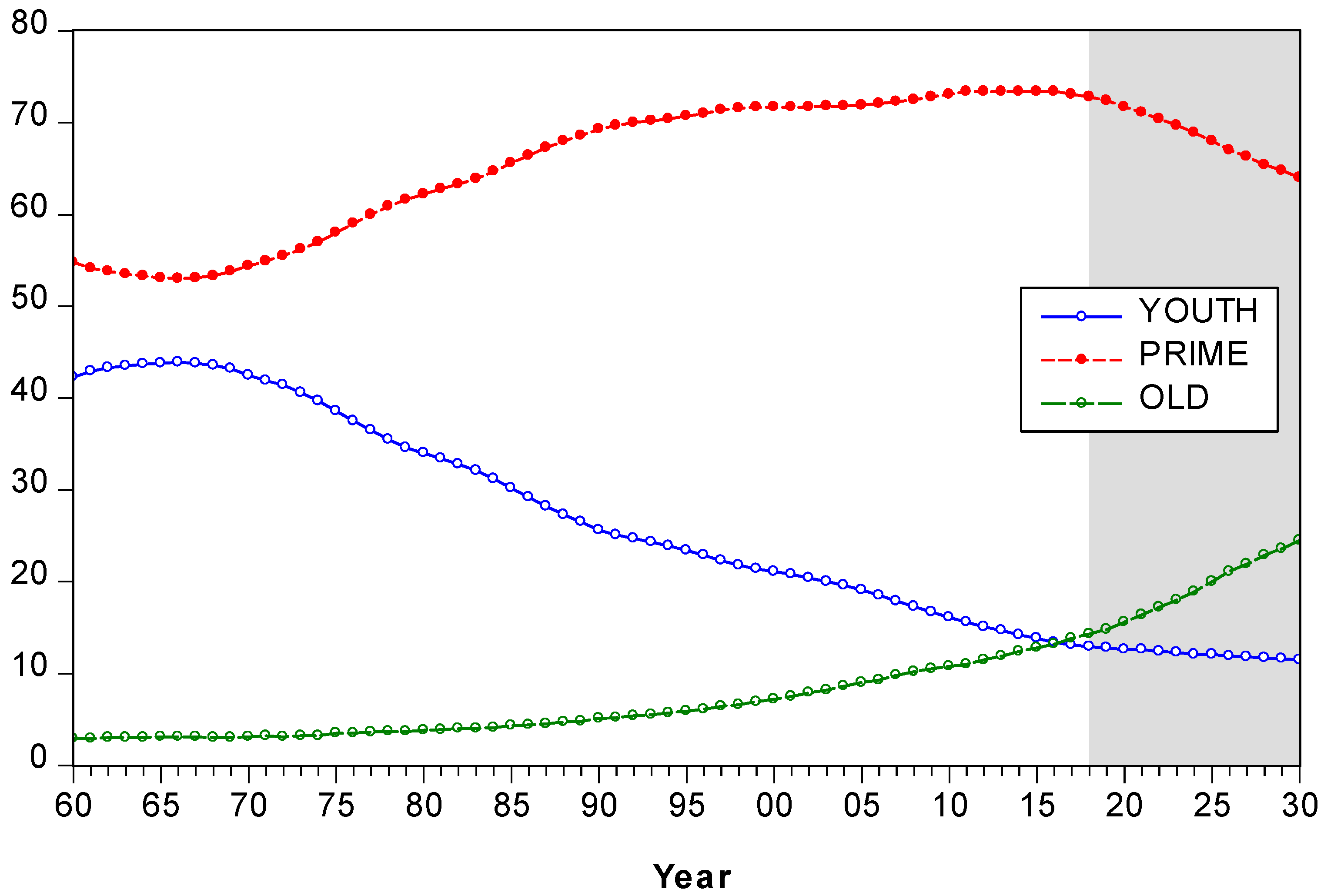
Korea, a newly developed economy, suffers from the same problem. Figure 1 shows the change in age structure of the Korean population [1]. The blue line indicates the proportion of the youth, aged 0 to 14, against the total population. The red line indicates the proportion of those in their prime, aged 15 to 64. The green line is the proportion of the old, aged 65 and over. A clear upward trend of the aging and a downward trend of the youth can be seen. The aging population has been continuously increasing; it comprised 13.8% of the total population in 2017. On the other hand, the share of the youth population began to decline from 1966, after reaching a peak of 43.9%. The prime age has also gradually increased until 2016, but begins to decline from 2017 after reaching a peak of 73.4%. The shaded area indicates expected values in the future, and we can see a sharp increase in the old and a sharp decrease in those in their prime. Korea had already become an aging society in 2000, and has become an aged society in 2017. The transition took only 17 years (According to the United Nations (UN) standards, an aging society is defined as a country in which the share of the population aged 65 and over exceeds 7% of the total population, and an aged society exceeds 14% of the total population). The problem is that this trend is extremely rapid relative to that of France (115 years), Germany (40 years), and the USA (73 years). It is widely acknowledged that population aging causes a shrinking labor force and large burdens on social security systems for the elderly, such as pension, health care and this can lead to poverty. These two issues are interconnected and trigger the overall macroeconomic problem. Economic growth can be slowed, not solely from a shrinking labor force, but also through consumption constraint. To deal with the rising burdens on social security systems, governments have to increase the tax rate. To make matters worse, in Korea, rising housing prices have lowered the marriage rate, which is affecting the fertility rate, and thus accelerating population aging.
According to the World Development Indicator, the fertility rate of Korea was recorded as 1.17 in 2016, which is the lowest in the world [33]. The government has been tackling these problems for a long time by introducing a series of policies. These policies mainly include childcare allowances, non-financial support for childcare, promotion of labor participation for women, and a reduced burden for newly married households. However, the results are not fruitful.
2.2. Energy Consumption in Korea
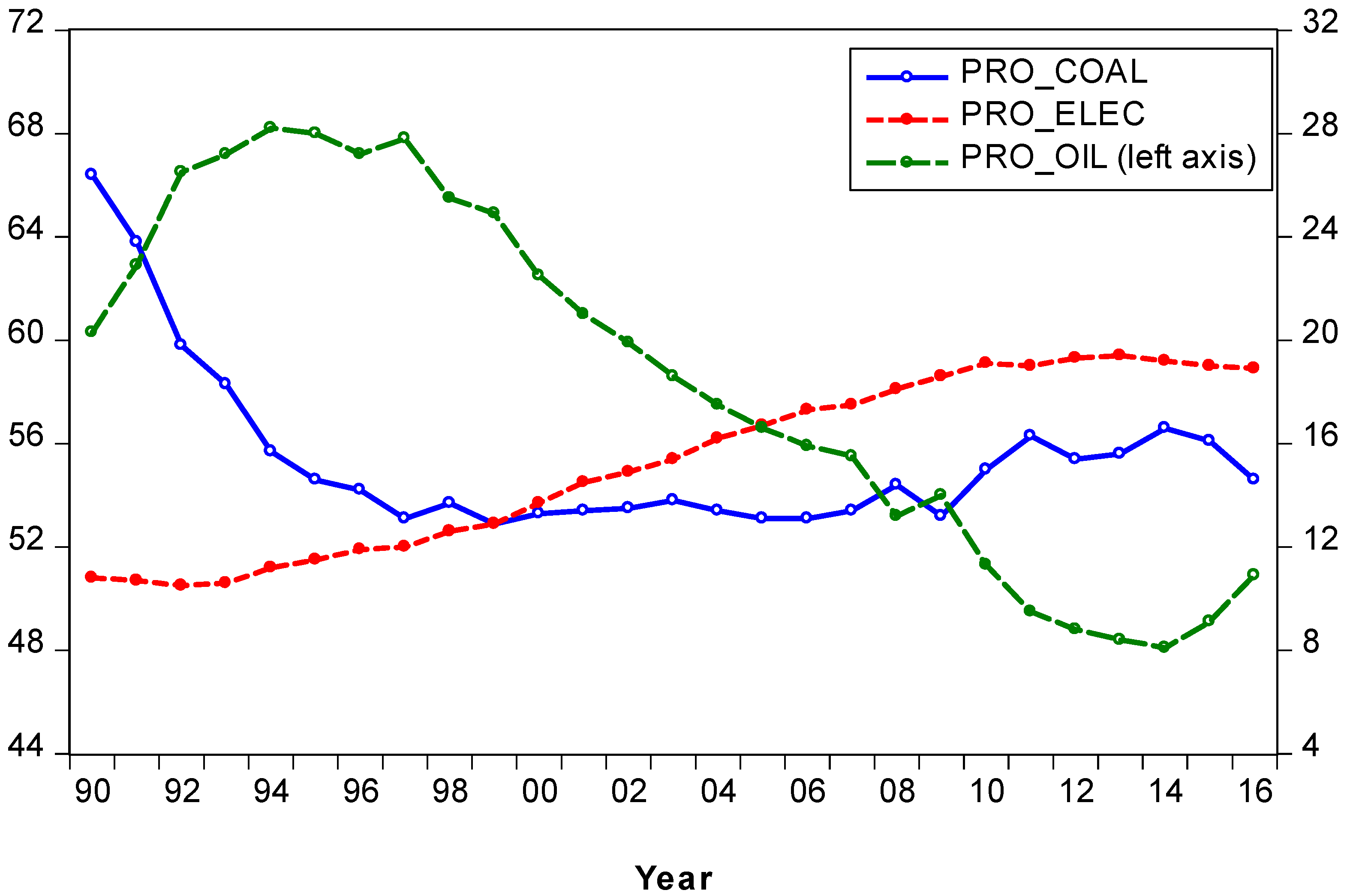
Due to the previously mentioned advantages of electricity, the demand for electricity has risen rapidly. Figure 2 shows the proportion of final energy consumption in Korea by its sources [34]. The green line (left axis) accounts for the oil consumption, and the blue and red lines (right axis) account for the coal and electricity consumption, respectively. In the past, oil and coal were the larger proportion, but as time went by, electricity consumption increased gradually. The graph shows the clear downward trend of oil, which reached its highest value of 68.2% in 1994 and declined to the lowest value of 48.1% in 2014, a huge drop of about 20%. Coal recorded 26.4% in 1990 but declined by 11.8% and ends up at 14.6%. Unlike the other two energy sources, electricity shows an upward trend. In 1990 electricity was only 10.8% of total final consumption, which was much less than coal consumption. However, it has increased gradually and was recorded as about 20% in 2016, which is almost double the 1990 value.
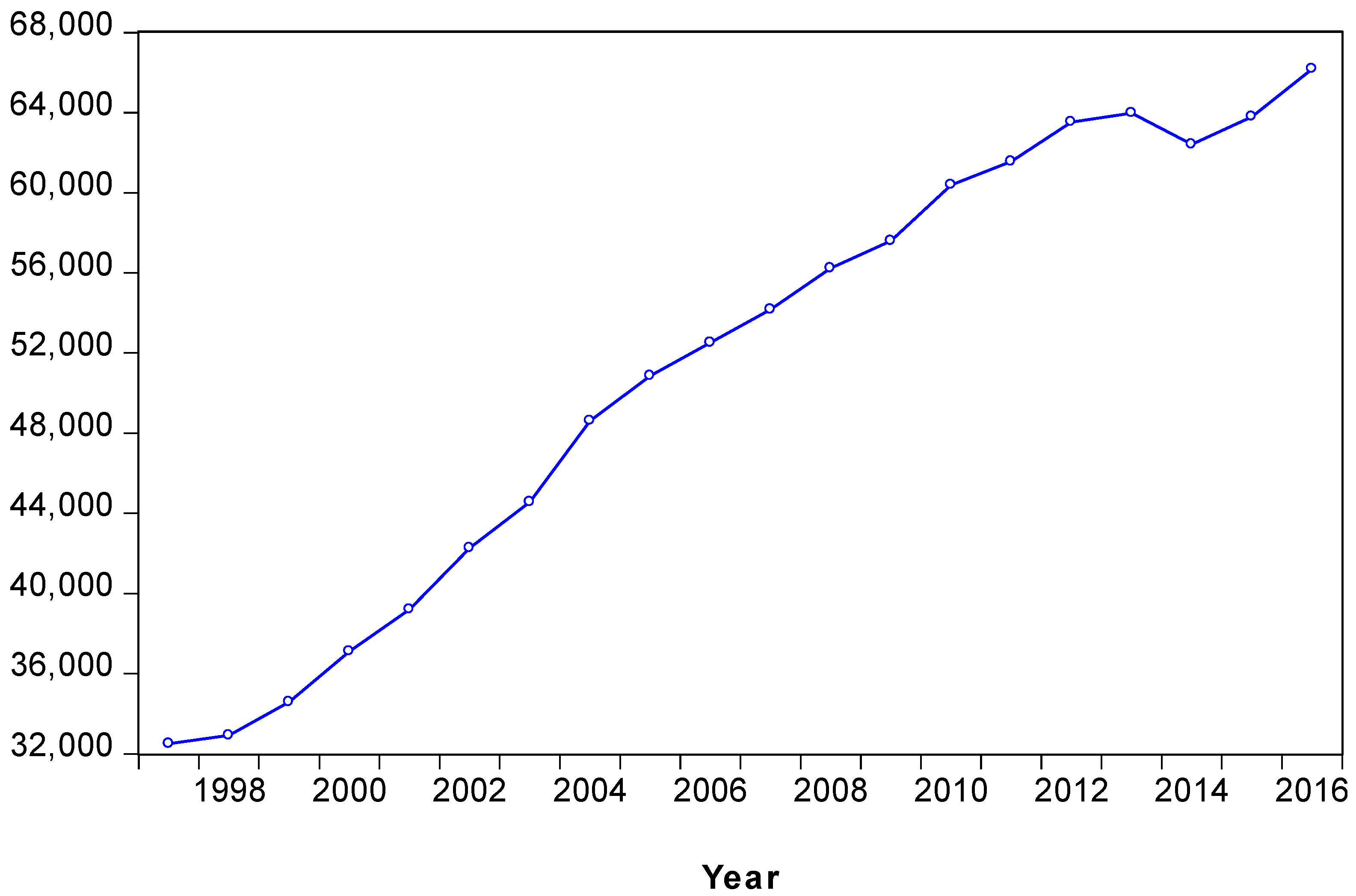
Figure 3 shows the residential electricity consumption in Korea [34]. In 1998, the consumption was about 32,000 GWh, and it grew continuously to around 66,000 GWh. It took 18 years for the residential electricity consumption to double. Many determinants played a role in this rapid increase. Among them, low electricity prices and climate change are considered to be important factors.
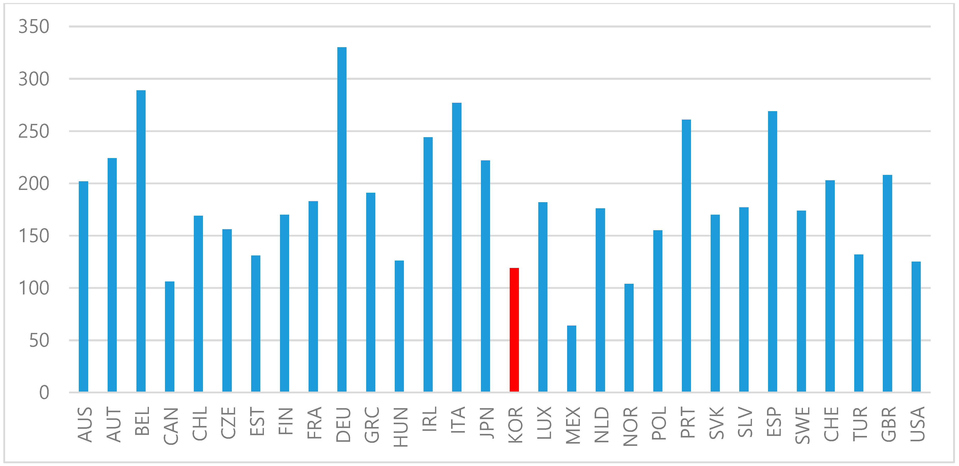
The International Energy Agency (IEA) [35] gives us the statistics of the residential electricity price for 30 OECD countries (Figure 4), and the Korean price is ranked at the 4th lowest level. The sample mean is approximately $185/MWh and the Korean price is $119/MWh. Even Japan, a neighbor of Korea, records $222/MWh, which is almost double.
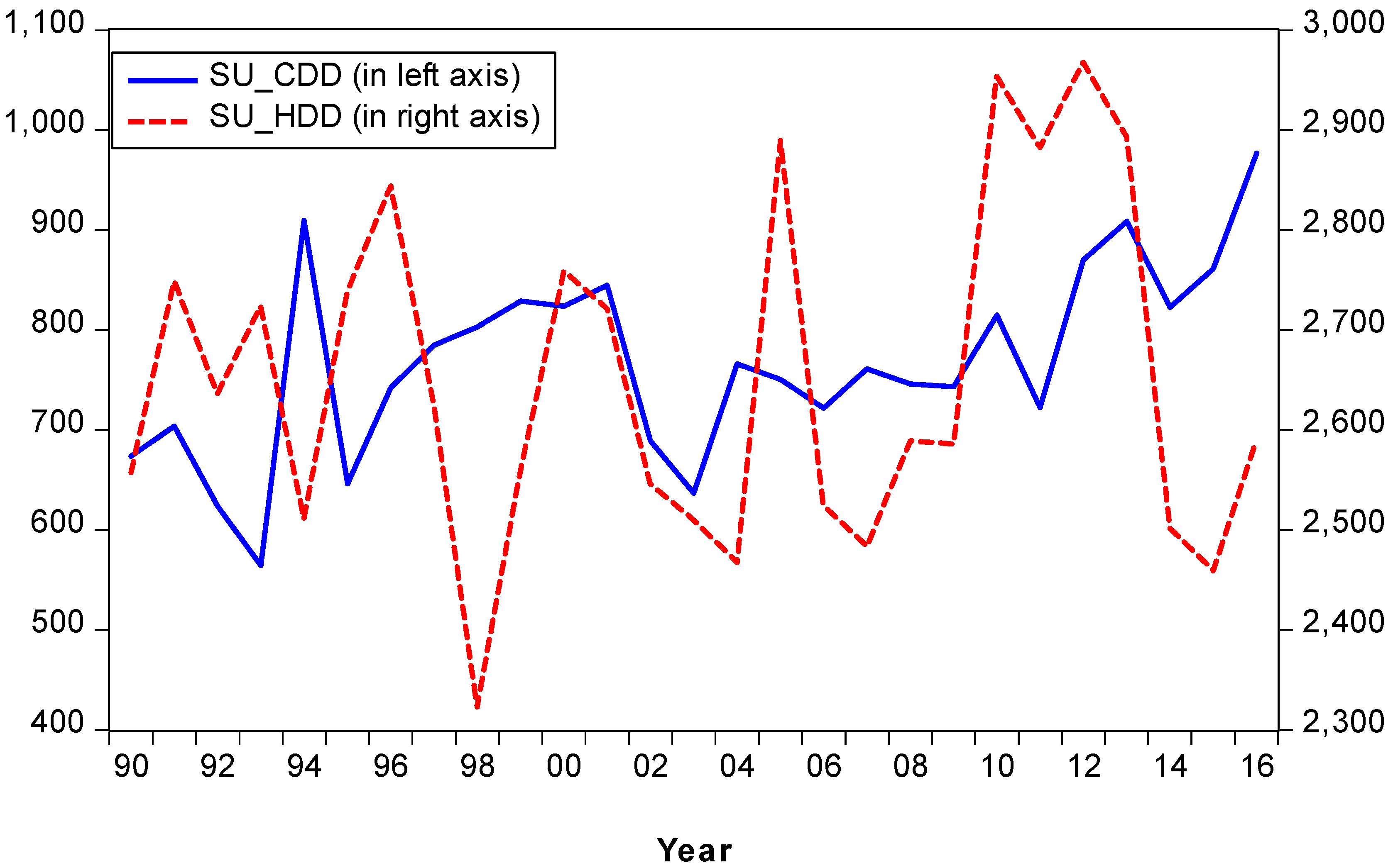
Climate conditions also push up the electricity demand. Figure 5 displays the cooling degree day (CDD) and heating degree day (HDD) in Seoul, the capital of Korea [36]. CDD and HDD are the most widely used indicators for quantifying energy demand for cooling and heating.
The higher the value, the greater the cooling and heating demands are. According to the statistics, CDD recorded 674 in 1990 and rose by 45% to 976 in 2016. HDD reached 2557 in 1990 and rose by 16% to 2967 in 2012. We can observe the upward trend in both indicators, although there are some fluctuations.
3. Econometric Methodology and Data Collection
3.1. Data Collection
Electricity is the major energy source for residential use in Korea. In this section, we discuss the effect of the population age structure and economic factors on residential electricity demand in Korea. For this study’s econometric model, the sixteen Korean provinces represent the individual units. The time-series for each unit has seventeen annual data points, for each year from 2000 to 2016, inclusive. Though we have Korean regional residential electricity consumption data from 1990, we only use the samples from 2000, based on three reasons. First, Korean provinces have been divided into sixteen regions since 1998 (Seoul, Busan, Daegu, Incheon, Gwangju, Daejon, Ulsan, Gyeonggi, Gangwon, Chungbuk, Chungnam, Jeonbuk, Jeonnam, Gyeongbuk, Gyeongnam and Jeju). Before 1998, Ulsan was a part of Gyeongnam, thus using the relevant data from those prior periods could distort the empirical results. Second, we only have the residential electricity consumption of Ulsan since 2000. Third, in the late 1990s, Korea experienced the Asian financial crisis and the liberalization of the oil market. Oil had been the primary energy source until these two major exogenous shocks caused an economic structural change. We finally estimate the FMOLS for long-run coefficients and the panel error correction model (PECM) for short-run coefficients based on the results of the panel unit-root and cointegration tests (For the same empirical analysis strategy in the field of energy economics, see Apergis and Payne [37,38]).
To discuss the effect of the population age structure and the economic factors on electricity demand, we consider the following model:
The data we use for the empirical analysis are divided into three groups. The first group is energy and economic variables, the second group is climate variables, and the third group is demographic variables. For the energy variables, we use residential electricity consumption (E), residential real electricity price (RP), and the consumer price index (CPI) for oil products (OP). For the economic variable, we use the real value (Y) of the gross regional domestic product (GRDP) in 2010. The data for regional residential electricity consumption is obtained from the Korea Energy Statistical Information System (KESIS) of Korean Energy Economics Institute (KEEI) [39]. We create the residential electricity price in real terms by deflating the nominal residential electricity price from the Korea Power Exchange (KPX) [40] by regional CPI obtained from the Korean Statistical Information Service (KOSIS) [41]. The CPI for oil products and GRDP are taken from the KOSIS [41,42] (In Korea, urban natural gas is widely used for heating, and can be a substitute for electricity. However, the regional level gas price is not available. Korea practically imports total fossil fuel from overseas, and the correlation between the national price level of oil and gas is over 0.96, so we have chosen the regional oil price for general substitutes).
We include the climate variables of heating degree day (HDD) and cooling degree day (CDD), which are taken from the Korea Meteorological Administration (KMA), to capture the temperature effect [36]. The demographic variables include the youth dependency ratio, the share of the population from ages 0 to 14 to prime age (P0014); old dependency ratio, over 65 to prime age (P65); old dependency ratio, between 65 and 79 to prime age (P6579); and old dependency ratio, over 80 to prime age (P80) (Ota et al. [13] include the fertility rate as an explanatory variable. We replace the fertility rate with the youth dependency ratio). They are obtained from the KOSIS [1]. In summary, we construct a balanced panel data set comprising 272 observations from 16 regions for the period 2000 to 2016.
3.2. Panel Unit Root and Cointegration Tests
In this section, we briefly introduce panel unit root and cointegration tests (For the overview of two econometric tests, see Baltagi [43] and Banerjee [44]). Because of the relatively long time-series information we have, the panel unit root test should be conducted. In this article, we consider three types of test which are most widely used, the IPS [45] test and Maddala-Wu Fisher-type augmented Dickey-Fuller (ADF) and Phillips-Perron (PP) tests [46]. The following Equation (2) is regression model for testing the unit root hypothesis.
The IPS test evaluates the null hypothesis, that each individual time series in the panel contains a unit root, against the alternative hypothesis that a non-zero fraction of the individual time series is stationary.
Maddala and Wu [27] propose an alternative way of testing the unit root hypothesis, Fisher-ADF and Fisher-PP test statistics, which combines the p-values from unit root tests for each individual i as follows.
Let pi be the asymptotic p-value of a unit root test for an individual time series i, and let P be the combination of the p-values. Note that P is distributed as a χ2 with 2N degrees of freedom as for finite N.
Verifying the existence of unit roots from the previous tests, we should conduct a panel cointegration test. Among various tests, we follow Pedroni [47,48] and Kao [49], the most widely used tests, to detect the long-run equilibrium relationship between these variables. The two tests are a residual-based cointegration test, which begins with the following spurious least square dummy variable (LSDV) regression model for the panel data (For the more detailed explanation of the two econometric tests, see Baltagi [43] and Banerjee [44]).
Kao [49] proposes a DF and ADF-type unit root test for as a test for the null of no cointegration. He shows that the asymptotic distributions of the test statistics converge to a Standard Normal by the sequential limit theorem. On the other hand, Pedroni [47,48] proposes several tests for cointegration that allows for heterogeneous individual effects and trend coefficients across each individual. Pedroni shows that the standardized statistic is asymptotically normally distributed.
3.3. Panel Cointegration Regression
In the empirical analysis with the panel data, the nonstationarity of the time series is an important issue for correct statistical inference. When all of the variables are cointegrated, we should estimate the long-run cointegration parameter, β from above Equation (4), to account for the nonstationarity property. For this reason, we employ the fully modified ordinary least squares (FMOLS) proposed by Pedroni [50]. He finds that the FMOLS estimator exhibits relatively minor size distortion in small samples and it is asymptotically unbiased for the standard case without intercepts, as well as the fixed effects model with heterogeneous intercepts [50]. Additionally, t-statistics for the FMOLS estimator of β from above Equation (4) is shown to be asymptotically standard normal.
3.4. Panel Error Correction Model
Following the seminal work of Engle and Granger [51], we specify the panel error correction model (PECM) to examine the short-run relationship between variables. After estimating Equation (2) by FMOLS, we estimate the PECM of the form:
where is the speed of adjustment coefficient and is called the error correction term (ECT). If shows a negative value with statistical significance, the PECM is well estimated.
4. Results
4.1. Long-Run Analysis
In this section, we discuss the results from above mentioned unit root and cointegration tests. Table 2 displays the p-value results from the three types of unit root tests. We take logarithms for all of the variables and the maximum lag structure is three, considering that the sample is in annual frequency. The unit root null hypothesis cannot reasonably be rejected under the 5% significance level, in the first and third group of variables, according to the IPS and the Maddala-Wu Fisher-type test. The second group of variables, HDD and CDD, are found to be stationary variables according to the same test. All the variables, besides HDD and CDD, are found to be I (1), integrated of order 1, according to the unit root test results in Table 2.
With the seven nonstationary variables, we test the cointegration hypothesis to identify the long-run relationship. We perform the previously mentioned Kao and Pedroni tests for these two groups of variables. Equation (6) is the test equation.
We use P65, P6579 and P80 for describing the OLD variable, however, the linear correlation between the three variables is 0.97. To avoid this problem, we combine E, RP, OP, Y, P0014 and P65 as Group 1, E, RP, OP, Y, P0014 and P6579 as Group 2 and E, RP, OP, Y, P0014 and P80 as Group 3. Table 3, Table 4 and Table 5 display the Pedroni’s cointegration test results and Table 6 shows the Kao’s. In the Pedroni test, 6 out of 11 statistics reject the null of no cointegration, and in the Kao test, the t-statistics reject the null for all the groups. Hence we reasonably conclude that the null of no cointegration can be rejected, and there is a long-run equilibrium relationship among variables.
Given the presence of a cointegration relationship, the FMOLS method is applied to determine the long-run relationship. Table 7 displays the long-run coefficient estimates of Equation (6) based on FMOLS.
Since all variables are expressed as natural logarithms, the coefficients are considered to represent elasticity. We firstly discuss the impact of the age structure variables. Estimation results show that a 1% increase in the youth dependency ratio increases residential electricity consumption by 0.87–0.89%; a 1% increase in the old age dependency ratio for individuals aged 65 and over increases the consumption by 0.45%; a 1% increase in the old age dependency ratio for individuals aged 65 to 79 increases consumption by 0.37%; on the other hand, a 1% increase in the old age dependency ratio for those aged 80 and over decreases residential electricity consumption by 0.1%. However, estimates of this old age dependency ratio for those aged 80 and over are not statistically significant. From the results, we can see that the youth population has a positive and a larger effect upon electricity demand than the old population. A possible explanation for the positive effect of youth on the electricity demand is the “Nintendo-effect” [30]. Children usually watch more TV, use PCs, and are heavy users of game devices.
Furthermore, children do not have enough money to spend outside the home to meet their needs. Additionally, population aging generally has a positive effect on residential electricity consumption. Previous studies support our results [10,11,21,22,25,26,27,28,29]. However, we verify that the effect is heterogeneous between old age groups. A possible explanation is that the elderly tend to stay at home longer, and are more concerned about heating and cooling.
Next, we discuss other non-demographic control variables. The results of Groups 1 to 3 indicate that a 1% increase in residential electricity price decreases residential electricity consumption by 0.57 to 0.64%; a 1% increase in oil price increases electricity consumption by 0.04% to 0.10%, which supports conventional economic theory of negative own-price effect and positive cross-price effect. Further, this could be evidence that electricity consumption is a substitute for overall fossil fuel consumption when the fossil fuel price increases. Both price elasticity is inelastic and cross-price elasticity is lower than own-price elasticity. We find that the results are similar to Zhou and Teng [26] in terms of own-price elasticity. In their article, using the annual urban household survey data of Sichuan Province in China from 2007 to 2009, own-price elasticity is found to be about -0.50%. In terms of cross-price elasticity, Ota et al. [13] show similar results. Using Japanese regional panel data, they include residential gas, whereas we include oil, as substitutes for electricity, yielding a cross-price elasticity of about 0.12.
For the income elasticity, we find that a 1% increase in real income leads to an increase in electricity consumption of 0.20%, 0.25% and 0.53%, respectively, which is inelastic. Compared with previous literature, our results are in the reasonable range. Zho and Teng [25] find that income elasticities are 0.14 to 0.34. Brounen et al. [30] show 0.11 based on Dutch household data and Ota et al. [13] show 0.08 for Japanese data. Estimated income elasticity from household survey data usually tends to be smaller than regional and macro data, since the effect is short-run. However, Liddle [27], applying the same method as ours based on twenty-two OECD countries, shows an income elasticity of 0.62.
4.2. Short-Run Analysis
According to the previous unit-root test, all of the variables are found to have nonstationary properties, except the climate variables. We should transform nonstationary variables into stationary variables by taking the natural log first difference. We further transform the climate variables in order to be consistent with the dependent variable. We estimate the following PECM model for short-run coefficients. The names and definitions of these variables have been explained previously in Section 3.1. The OLD variable represents P65, P6579 and P80 and the ECT variable represents the error correction term generated by Equation (6).
We additionally change the Equation (7) slightly to Equation (8) by dividing the residential electricity price by the oil price in order to reflect the relative price effect.
Models 1 to 6 in Table 8 show the estimation results of PECM. All of the variables are log differenced, and 240 observations are used. We apply robust standard error clustered by individual cross-section. First of all, the sign of ECT is negative and statistically significant, which means the error correction model is functioning well.
The overall result is qualitatively in line with previously estimated long-run elasticities. Among the population age structure variables, the youth dependency ratio, P0014, shows positive values between 0.56–0.72, which are statistically significant under the 1% significance level. Since all the variables are log-difference transformed, we can interpret that a 1%p increase in P0014 leads to a 0.56-0.72%p increase in residential electricity consumption, which is a marginal effect. The “Nintendo-effect” could be a good explanation for the result [30].
The estimated coefficients of the old age dependency ratio, P65 and P6579 show a positive value, 0.34 and 0.26, respectively, which could be interpreted as a 0.34%p and 0.26%p increase in residential electricity consumption as a result of a 1%p increase in P65 and P6579, respectively. However, another dependency ratio of those aged over 80 to those of prime age, P80, shows statistically insignificant estimates. Therefore, we can infer that people aged 65 and over in Korea generally have higher residential electricity usage. However, when we divide the old age group more specifically, it is hard to conclude that people aged 80 and over have no effect on the residential electricity demand.
Next, we discuss the control variables. The estimated coefficient of the income variable, Y, is 0.26 to 0.36, and is statistically significant under the 1% level for all the models. The estimated coefficient, interpreted as the marginal effect of income on electricity demand, indicates that a 1%p increase in income leads to a 0.26 to 0.36%p increase in residential electricity demand. The residential electricity price, RP, shows negative estimates of −0.11 and −0.14 in Model 1 and Model 5, and is statistically significant under the 5% level. The oil price, OP, as the general fossil fuel price, shows a positive sign and is statistically significant under the 1% level in Models 1, 3 and 5. In Models 2, 4 and 6, representing the own-price variable to cross-price variable, the sign of the electricity variable becomes negative under the 1% significance level. These overall effects of price variables support economic theory, thus we conclude that the models are well constructed. The estimated coefficients of HDD and CDD have similar magnitudes of around 0.03 to 0.05, which are positive and significant at least under the 10% level.
4.3. Robustness
This section considers robustness checks. We consider robustness to alternative population age structure variables. In previous empirical analysis, we include P0014, P65, P6579 and P80 to represent the age structure. All of these three variables are divided by the prime age group in order to capture the relative effects. However, according to a few existing studies, we use more direct age structure variables as alternatives [13,19,29]. A0014 refers to the share in the total population of the youth aged between 0 to 14 years; O65, O6579 and O80 are the share of the population aged 65 and over, 65 to 80 and 80 and over, respectively.
We use the same procedure of panel unit-root and cointegration tests, and we can conclude that there is a long-run equilibrium relationship among existing and newly introduced age structure variables (Unit-root and cointegration tests results can be provided upon request). The robustness of the long-run and short-run coefficients is summarized in Table 9; Table 10.
The results are qualitatively the same as the previous estimation in Section 4.1 and Section 4.2 in which we conclude that the population age structure effect is robust for residential electricity consumption. Even so, we can find statistical improvements in Table 10. The adjusted-R2 in Models 5 to 10 is about 0.60, which is a slight improvement over the previous value of 0.57 in Models 1 to 6. Further, O80, the share of people aged 80 and over, is statistically significant under the 10% level, whereas in Models 5 and 6, the coefficients of P80 are not statistically significant. Thus, we may address that people aged 80 and over may weakly raise residential electricity consumption in the short-run in terms of statistical significance, but its magnitude is smaller than for people aged 65 and over.
5. Conclusions and Policy Implications
Korea has been facing critical demographic issues with regard to population aging. In addition, a growing trend towards sustainable growth sheds light on the energy policy in Korea. In the present study, we analyze the effects of the population age structure on the residential electricity demand by using Korean panel data at the regional level. Our empirical analysis has shown clear evidence of age structure effects on residential electricity consumption that would provide important economic implications for energy and industrial policy.
When it comes to the population age structure’s effects, we find that an increase in both the youth dependency ratio and the old age dependency ratio, over 65 to prime, lead to an increase in residential electricity consumption in the short- and long-run. We further divide the group of people aged 65 and over into two groups, those aged 65 to 79 and 80 and over, to investigate the heterogeneous age structure effect. We also find a positive impact of people aged between 65 and 79 to prime on the residential electricity demand. On the other hand, an increase in the old age dependency ratio, over 80 to prime age, generally has no effect on residential electricity consumption.
We can conclude that people aged 65 and over in Korea generally use more electricity when compared to the prime age population, despite a heterogeneous effect from different old age groups, because old people tend to stay home longer and are concerned more about heating and cooling to maintain their health.
The results documented in this paper have important policy implications. Korea declared that it will reduce its greenhouse gases (GHGs) by 37% from the business as usual levels by 2030. The growth of the residential electricity demand is accelerated by the youth and old population with the growth in heating and cooling demands, and this would be a barrier for the NDC goal (Pezzutto et al. [52] find that energy consumption for air conditioning steadily increases over the past two decades in Europe. And they expect positive growth in space cooling market due to the increase in comfort requests by the European population concerning climatic well-being in dwellings and workplaces). Statistics Korea, the Korean statistics authority, predicts that the share of old people will be continuously increasing, reaching 24.5% in 2030 and 32.8% in 2040 [1]. Based on our empirical results, this trend could raise the residential electricity consumption with corresponding negative effects on GHGs. Demographic factors might be considered in forecasting future economic activities for calculating the NDC goal; however, the behavioral pattern of the aged population should be also considered for future energy policies.
Significantly increasing the supply of electricity from renewable sources could be a major solution in the era of an aging society. The Korean government aims to enhance renewable energy towards the year 2030 through the recently established National Renewable Energy Plan. However, the pace of renewable energy deployment in Korea is quite slow. The BP Statistical Review of World Energy 2017 reports that installed photovoltaic (PV) power and wind turbine cumulatively provide 4350 MW and 1089 MW respectively in Korea [53]. These capacities are far behind those of Japan and most advanced European countries. The World Development Indicator also shows that only 1% of electricity production is from renewable sources, excluding hydroelectric [54].
Additionally, energy efficiency improvement policies, such as weatherization programs, seem to be appropriate policies for the older generation to reduce electricity consumption in Korea, since enhancing the renewable energy capacity may not be implemented in the short-run [55]. The OECD report states that the old-age income poverty of Korea reached 45.7% in the latest statistics, which is the highest level among OECD countries [56]. Considering that the average old-age income poverty rate in OECD countries is 12.5%, the value is about three times higher. Furthermore, the old generation only earns 69% of the average income in Korea, which is a very low value compared to 87.6%, the average of OECD members [56]. This old-age income poverty could be a liquidity constraint for switching the existing facilities to more efficient ones. Considering that one of the prominent reasons that old people consume more electricity is heating and cooling for their health, supporting such energy efficiency improvements could help reduce domestic energy consumption. Local governments have been supporting the improvement of energy efficiency, but nation-wide and more sophisticated policies will be needed to address the energy efficiency improvement for old people.
Author Contributions
Formal analysis, writing—original draft, supervision, J.K.; data curation, writing—review & editing; M.J.; methodology, D.S.
Funding
This research was supported by the Korea Energy Economics Institute.
Acknowledgments
We would like to thank the anonymous reviewers for their valuable comments.
Conflicts of Interest
The authors declare no conflict of interest.
References
- Korean Statistical Information Service (KOSIS). Population Projections and Summary Indicator. Available online: http://kosis.kr/statHtml/statHtml.do?orgId=101&tblId=DT_1BPB003&conn_path=I3 (accessed on 13 February 2019).
- World Development Indicator. Population Ages 65 and Above (% of Total). Available online: https://data.worldbank.org/indicator/SP.POP.65UP.TO.ZS (accessed on 6 December 2017).
- Bloom, D.E.; Canning, D.; Fink, G. Implications of population ageing for economic growth. Oxf. Rev. Econ. Policy 2010, 26, 583–612. [Google Scholar] [CrossRef] [Green Version]
- Fair, R.C.; Dominguez, K.M. Effects of the changing US age distribution on macroeconomic equations. Am. Econ. Rev. 1991, 81, 1276–1294. Available online: jstor.org/stable/2006917 (accessed on 30 November 2017).
- Higgins, M. Demography, national savings, and international capital flows. Int. Econ. Rev. 1998, 39, 343–369. Available online: jstor.org/stable/2527297 (accessed on 2 October 2018). [CrossRef]
- Arnott, R.D.; Chaves, D.B. Demographic changes, financial markets, and the economy. Financ. Anal. J. 2012, 68, 23–46. [Google Scholar] [CrossRef]
- Gajewski, P. Is ageing deflationary? Some evidence from OECD countries. Appl. Econ. Lett. 2015, 22, 916–919. [Google Scholar] [CrossRef]
- Imam, P.A. Shock from graying: Is the demographic shift weakening monetary policy effectiveness. Int. J. Financ. Econ. 2015, 20, 138–154. [Google Scholar] [CrossRef]
- Juselius, M.; Takáts, E. Can demography affect inflation and monetary policy? Available online: https://ssrn.com/abstract=2562443 (accessed on 27 November 2017).
- Bardazzi, R.; Pazienza, M.G. Switch off the light, please! Energy use, aging population and consumption habits. Energy Econ. 2017, 65, 161–171. [Google Scholar] [CrossRef]
- Elnakat, A.; Gomez, J.D.; Booth, N. A zip code study of socioeconomic, demographic, and household gendered influence on the residential energy sector. Energy Rep. 2016, 2, 21–27. [Google Scholar] [CrossRef] [Green Version]
- Fu, C.; Wang, W.; Tang, J. Exploring the sensitivity of residential energy consumption in China: Implications from a micro-demographic analysis. Energy Res. Soc. Sci. 2014, 2, 1–11. [Google Scholar] [CrossRef]
- Ota, T.; Kakinaka, M.; Kotani, K. Demographic effects on residential electricity and city gas consumption in the aging society of Japan. Energy Policy 2018, 115, 503–513. [Google Scholar] [CrossRef] [Green Version]
- Cole, M.A.; Neumayer, E. Examining the impact of demographic factors on air pollution. Popul. Environ. 2004, 26, 5–21. [Google Scholar] [CrossRef]
- Dalton, M.; o’Neill, B.; Prskawetz, A.; Jiang, L.; Pitkin, J. Population aging and future carbon emissions in the United States. Energy Econ. 2008, 30, 642–675. [Google Scholar] [CrossRef] [Green Version]
- Fan, Y.; Liu, L.C.; Wu, G.; Wei, Y.M. Analyzing impact factors of CO2 emissions using the STIRPAT model. Environ. Impact Assess. Rev. 2006, 26, 377–395. [Google Scholar] [CrossRef]
- Kronenberg, T. The impact of demographic change on energy use and greenhouse gas emissions in Germany. Ecol. Econ. 2009, 68, 2637–2645. [Google Scholar] [CrossRef]
- Liddle, B.; Lung, S. Age-structure, urbanization, and climate change in developed countries: Revisiting STIRPAT for disaggregated population and consumption-related environmental impacts. Popul. Environ. 2010, 31, 317–343. [Google Scholar] [CrossRef]
- Menz, T.; Kühling, J. Population aging and environmental quality in OECD countries: Evidence from sulfur dioxide emissions data. Popul. Environ. 2011, 33, 55–79. [Google Scholar] [CrossRef]
- Menz, T.; Welsch, H. Population aging and carbon emissions in OECD countries: Accounting for life-cycle and cohort effects. Energy Econ. 2012, 34, 842–849. [Google Scholar] [CrossRef]
- Roberts, S. Demographics, energy and our homes. Energy Policy 2008, 36, 4630–4632. [Google Scholar] [CrossRef]
- Tonn, B.; Eisenberg, J. The aging US population and residential energy demand. Energy Policy 2007, 35, 743–745. [Google Scholar] [CrossRef]
- Ahn, Y.; Chae, Y. Analyzing spatial equality of cooling service shelters, central district of Seoul metropolitan city, South Korea. Spat. Inf. Res. 2018, 26, 619–627. [Google Scholar] [CrossRef]
- Kayaba, M.; Kondo, M.; Honda, Y. Characteristics of elderly people living in non-air-conditioned homes. Environ. Health Prev. Med. 2015, 71, 68–71. [Google Scholar] [CrossRef] [PubMed]
- Zhou, S.; Teng, F. Estimation of urban residential electricity demand in China using household survey data. Energy Policy 2013, 61, 394–402. [Google Scholar] [CrossRef]
- Kim, J.; Seo, B. Aging in population and energy demand. In Proceedings of the 3rd IAEE Asian Conference, Kyoto, Japan, 20–22 February 2012; pp. 66–78. [Google Scholar]
- Liddle, B. Consumption-driven environmental impact and age structure change in OECD countries: A cointegration-STIRPAT analysis. Dem. Res. 2011, 24, 749–770. [Google Scholar] [CrossRef]
- Yamasaki, E.; Tominaga, N. Evolution of an aging society and effect on residential energy demand. Energy Policy 1997, 25, 903–912. [Google Scholar] [CrossRef]
- York, R. Demographic trends and energy consumption in European Union Nations, 1960–2025. Soc. Sci. Res. 2007, 36, 855–872. [Google Scholar] [CrossRef]
- Brounen, D.; Kok, N.; Quigley, J.M. Residential energy use and conservation: Economics and demographics. Eur. Econ. Rev. 2012, 56, 931–945. [Google Scholar] [CrossRef]
- Garau, G.; Lecca, P.; Mandras, G. The impact of population ageing on energy use: Evidence from Italy. Econ. Model 2013, 35, 970–980. [Google Scholar] [CrossRef]
- Ministry of Trade, Industry and Energy (MOTIE). The 8th Basic Plan for Long-term Electricity Supply and Demand (2017–2031); Ministry of Trade, Industry and Energy: Sejong City, Korea, 2017.
- World Development Indicator. Fertility Rate, Total (Births per Woman). Available online: https://data.worldbank.org/indicator/SP.DYN.TFRT.IN (accessed on 10 July 2019).
- Korea Energy Economics Institute (KEEI). 2018 Yearbook of Energy Statistics, December 2018 ed.; Korea Energy Economics Institute: Ulsan, Korea, 2018. [Google Scholar]
- IEA. Key World Energy Statistics 2017; International Energy Agency Publications: Paris, France, 2017. [Google Scholar]
- Korea Meteorological Administration (KMA). Temperature Analysis. Available online: https://data.kma.go.kr/stcs/grnd/grndTaList.do?pgmNo=70 (accessed on 29 April 2018).
- Apergis, N.; Payne, J.E. Renewable energy consumption and economic growth: Evidence from a panel of OECD countries. Energy Policy 2010, 38, 656–660. [Google Scholar] [CrossRef]
- Apergis, N.; Payne, J.E. Renewable and non-renewable energy consumption-growth nexus: Evidence from a panel error correction model. Energy Econ. 2012, 34, 733–738. [Google Scholar] [CrossRef]
- Korea Energy Statistical Information System (KESIS). Electricity Consumption by Region and Industry. Available online: http://www.kesis.net/sub/sub_0001_eng.jsp (accessed on 17 January 2018).
- Korea Power Exchange (KPX). Power Exchange Main Screen / Trusted Power Business Platform. Available online: http://www.kpx.or.kr (accessed on 12 January 2018).
- Korean Statistical Information Service (KOSIS). Annual CPI by Commodities & Services. Available online: http://kosis.kr/statHtml/statHtml.do?orgId=101&tblId=DT_1J15136&conn_path=I3 (accessed on 28 December 2017).
- Korean Statistical Information Service (KOSIS). Regional Income. Available online: http://kosis.kr/statHtml/statHtml.do?orgId=101&tblId=DT_1BPB003&conn_path=I3 (accessed on 28 December 2017).
- Baltagi, B.H. Econometric Analysis of Panel Data, 4th ed.; John Wiley & Sons Ltd.: Chichester, UK, 2008; pp. 273–310. ISBN 978-0-470-51886-1. [Google Scholar]
- Banerjee, A. Panel data unit roots and cointegration: An overview. Oxf. Bull. Econ. Stat. 1999, 61, 607–629. [Google Scholar] [CrossRef]
- Im, K.S.; Pesaran, M.H.; Shin, Y. Testing for unit roots in heterogeneous panels. J. Econ. 2003, 115, 53–74. [Google Scholar] [CrossRef]
- Maddala, G.S.; Wu, S. A comparative study of unit root tests with panel data and a new simple test. Oxf. Bull. Econ. Stat. 1999, 61, 631–652. [Google Scholar] [CrossRef]
- Pedroni, P. Critical values for cointegration tests in heterogeneous panels with multiple regressors. Oxf. Bull. Econ. Stat. 1999, 61, 653–670. [Google Scholar] [CrossRef]
- Pedroni, P. Panel cointegration: Asymptotic and finite sample properties of pooled time series tests with an application to the PPP Hypothesis. Econ. Theory 2004, 20, 597–625. [Google Scholar] [CrossRef]
- Kao, C. Spurious regression and residual-based test for cointegration in panel data. J. Econ. 1999, 90, 1–44. [Google Scholar] [CrossRef]
- Pedroni, P. Fully modified OLS for heterogeneous cointegrated panels. In Nonstationary Panels, Panel Cointegration, and Dynamic Panels (Advances in Econometrics); Baltagi, B.H., Fomby, T.B., Hill, R.C., Eds.; Emerald Group Publishing Ltd.: Bingley, UK, 2001; Volume 15, pp. 93–130. [Google Scholar]
- Engle, R.F.; Granger, C.W.J. Co-integration and error correction: Representation, estimation, and testing. Econometrica 1987, 55, 251–276. Available online: jstor.org/stable/1913236 (accessed on 5 February 2013). [CrossRef]
- Pezzutto, S.; Fazeli, R.; De Felice, M.; Sparber, W. Future development of the air-conditioning market in Europe: An outlook until 2020. WIREs Energy Environ. 2016, 5, 649–669. [Google Scholar] [CrossRef]
- BP Statistical Review of World Energy 2017. Available online: http://www.bp.com/statisticalreview (accessed on 16 June 2018).
- World Development Indicator. Electricity Production from Renewable Sources, Excluding Hydroelectric (% of Total). Available online: https://data.worldbank.org/indicator/EG.ELC.RNWX.ZS (accessed on 6 December 2017).
- Hamza, N.; Gilroy, R. The challenge to UK energy policy: An ageing population perspective on energy saving measures and consumption. Energy Policy 2011, 39, 782–789. [Google Scholar] [CrossRef]
- OECD. Pensions at a Glance 2017: OECD and G20 Indicators; OECD Publishing: Paris, France, 2017. [Google Scholar] [CrossRef]
Figure 1.
Population Age Structure in Korea. (% of total population).

Figure 2.
Proportion of Energy Consumption in Korea (% of total energy consumption).

Figure 3.
Residential Electricity Consumption in Korea (GWh).

Figure 4.
Residential Electricity Price of Organisation for Economic Co-operation and Development (OECD) countries. ($/MWh).
Figure 4.
Residential Electricity Price of Organisation for Economic Co-operation and Development (OECD) countries. ($/MWh).

Figure 5.
Cooling degree days (CDDs) and heating degree days (HDDs) in Seoul.

Figure 6.
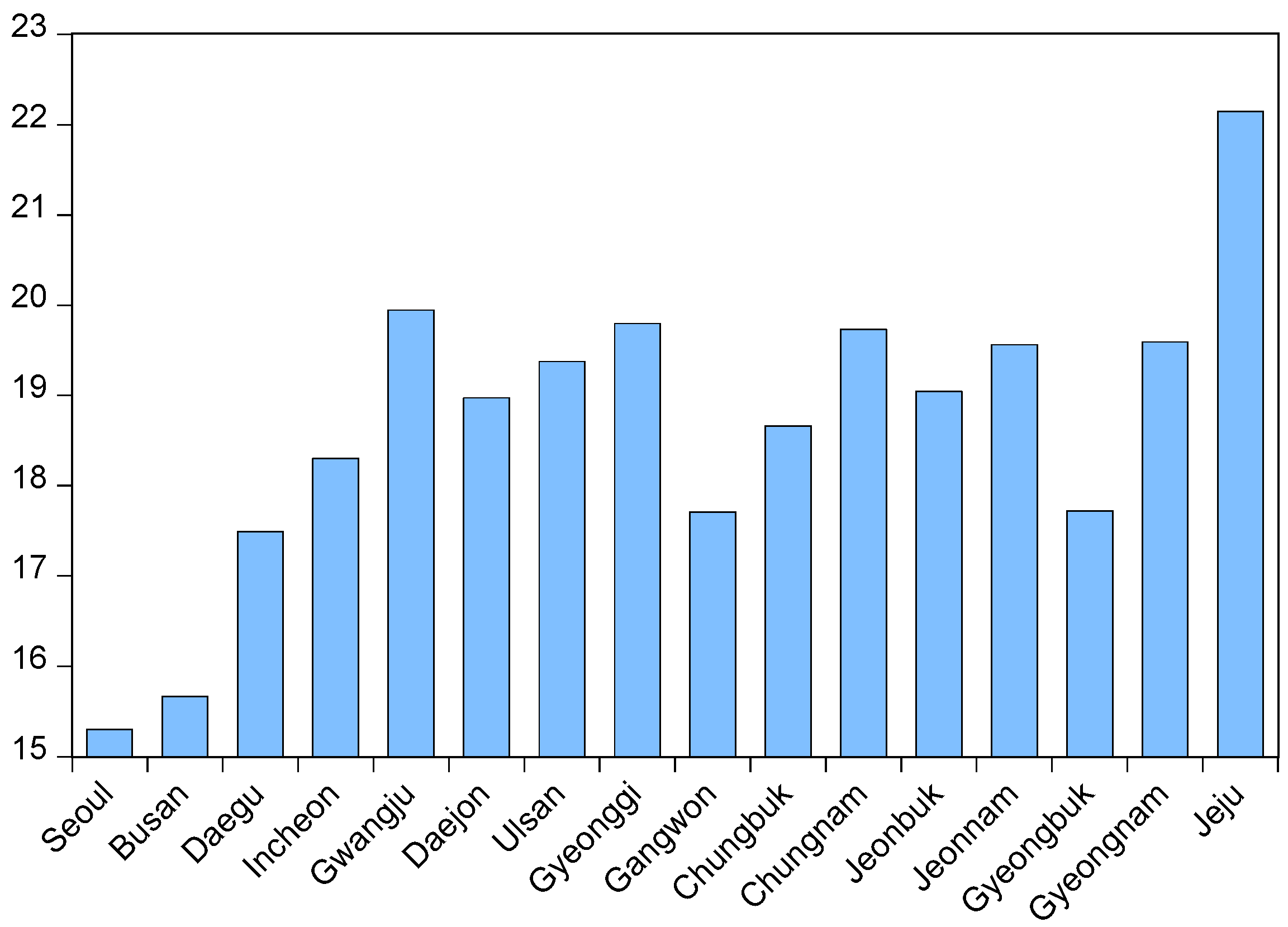
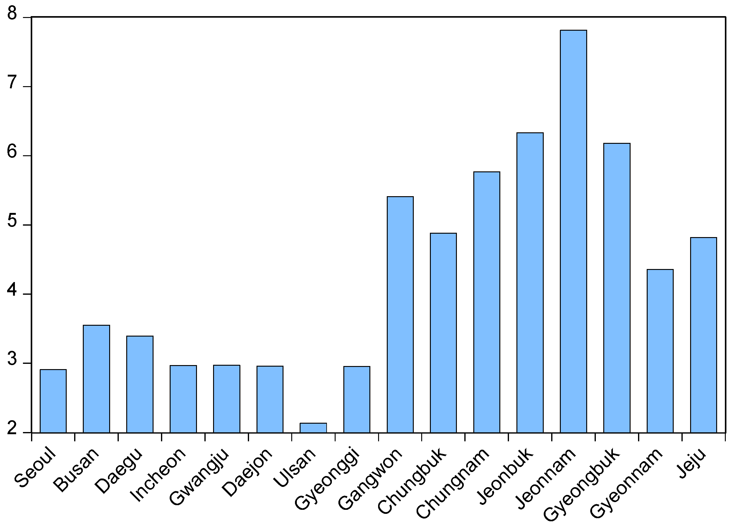
Youth dependency ratio for each region in 2016.

Figure 7.
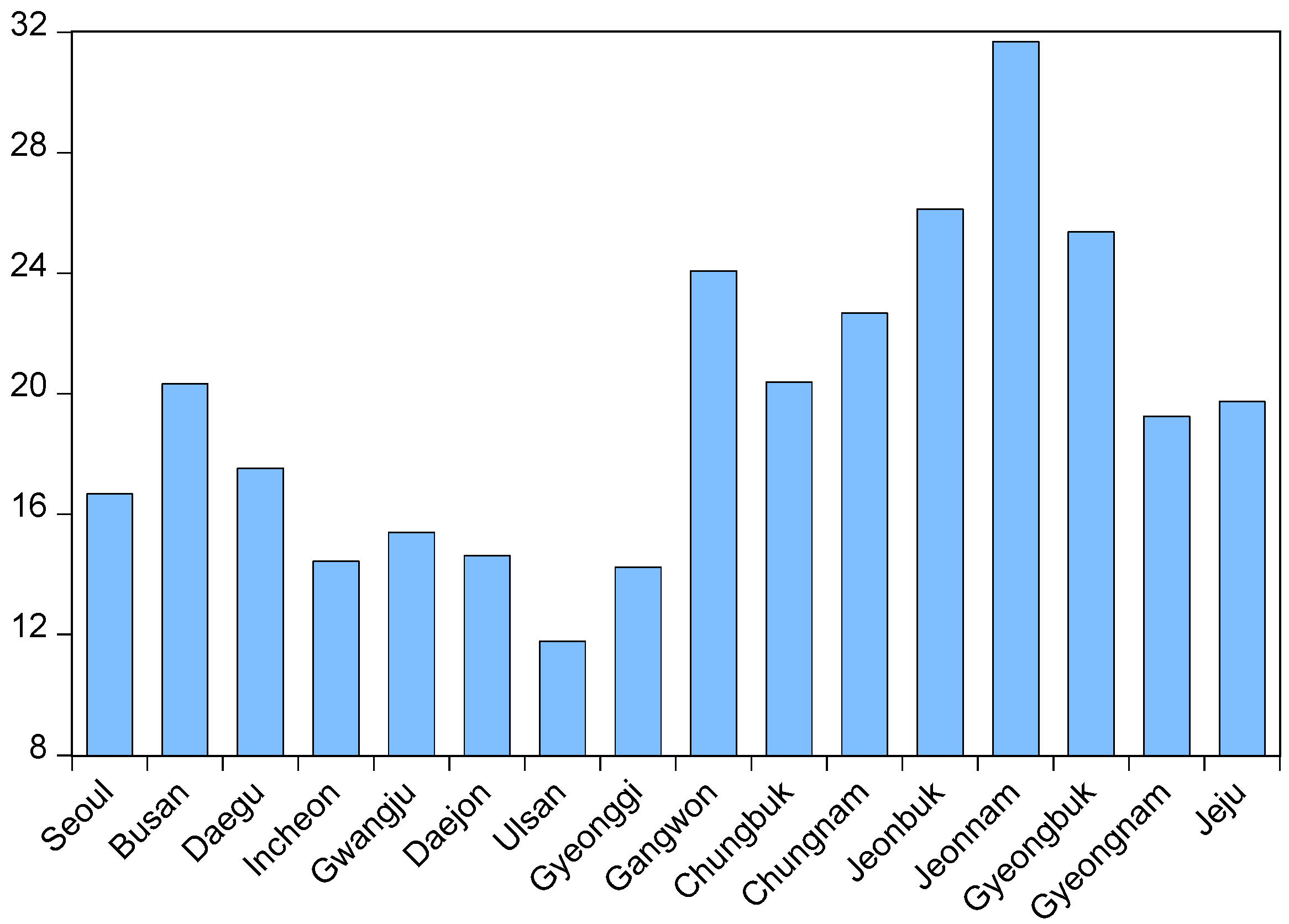
Old dependency ratio, over 65, for each region in 2016.

Figure 8.
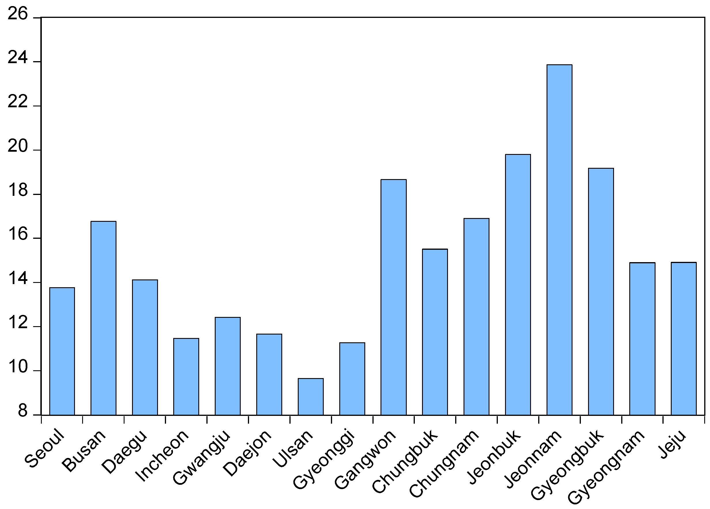
Old dependency ratio, 65 to 79, for each region in 2016.

Figure 9.
Old dependency ratio, over 80, for each region in 2016.


Table 1.
Summary statistics (Observations = 272).
| Category | Var | Mean | Std. Dev | Skewness | Kurtosis | Source |
|---|---|---|---|---|---|---|
| Energy | E | 7.78 | 0.78 | 0.58 | 3.60 | KESIS |
| Economy | RP | 0.31 | 0.09 | 0.42 | 2.04 | KPX |
| OP | 4.58 | 0.21 | −0.11 | 1.79 | KOSIS | |
| Y | 17.75 | 0.80 | 0.40 | 3.33 | ||
| Climate | HDD | 7.76 | 0.19 | −0.62 | 2.94 | KMA |
| CDD | 6.64 | 0.16 | −0.42 | 3.43 | ||
| Age Structure | P0014 | 3.19 | 0.19 | −0.23 | 2.21 | KOSIS |
| P65 | 2.68 | 0.39 | −0.16 | 2.20 | ||
| P6579 | 2.49 | 0.37 | −0.19 | 2.22 | ||
| P80 | 0.90 | 0.50 | −0.03 | 2.23 |
Table 2.
Unit root test results.
| Var | IPS | Fisher-ADF | Fisher-PP |
|---|---|---|---|
| E | 0.99 | 1.00 | 0.99 |
| ΔE | 0.00 | 0.00 | 0.00 |
| RP | 0.99 | 1.00 | 0.72 |
| ΔRP | 0.00 | 0.00 | 0.00 |
| OP | 0.38 | 0.83 | 0.82 |
| ΔOP | 0.00 | 0.00 | 0.00 |
| Y | 0.64 | 0.34 | 0.00 |
| ΔY | 0.00 | 0.00 | 0.00 |
| HDD | 0.00 | 0.00 | 0.00 |
| CDD | 0.00 | 0.00 | 0.00 |
| P0014 | 1.00 | 0.99 | 1.00 |
| ΔP0014 | 0.00 | 0.00 | 0.00 |
| P65 | 0.16 | 0.10 | 0.99 |
| ΔP65 | 0.00 | 0.00 | 0.01 |
| P6579 | 0.98 | 0.94 | 0.99 |
| ΔP6579 | 0.00 | 0.00 | 0.00 |
| P80 | 1.00 | 1.00 | 0.97 |
| ΔP80 | 0.00 | 0.00 | 0.00 |
Table 3.
Pedroni cointegration test results for Group 1.
| Types | Statistics | p-Value | Weighted Statistics | p-Value |
|---|---|---|---|---|
| Panel v | 0.46 | 0.32 | −0.38 | 0.65 |
| Panel rho | 3.43 | 0.99 | 3.46 | 0.99 |
| Panel PP | −5.05 | 0.00 | −5.36 | 0.00 |
| Panel ADF | −3.37 | 0.00 | −3.64 | 0.00 |
| Group rho | 5.37 | 0.99 | ||
| Group PP | −8.67 | 0.00 | ||
| Group ADF | −3.16 | 0.00 |
Table 4.
Pedroni cointegration test results for Group 2.
| Types | Statistics | p-Value | Weighted Statistics | p-Value |
|---|---|---|---|---|
| Panel v | 0.35 | 0.36 | −1.25 | 0.89 |
| Panel rho | 3.30 | 0.99 | 3.36 | 0.99 |
| Panel PP | −4.78 | 0.00 | −6.01 | 0.00 |
| Panel ADF | −3.49 | 0.00 | −3.44 | 0.00 |
| Group rho | 5.11 | 1.00 | ||
| Group PP | −9.90 | 0.00 | ||
| Group ADF | −3.49 | 0.00 |
Table 5.
Pedroni cointegration test results for Group 3.
| Types | Statistics | p-Value | Weighted Statistics | p-Value |
|---|---|---|---|---|
| Panel v | 0.80 | 0.21 | −0.77 | 0.78 |
| Panel rho | 2.06 | 0.98 | 1.83 | 0.97 |
| Panel PP | −8.07 | 0.00 | −7.31 | 0.00 |
| Panel ADF | −5.58 | 0.00 | −5.59 | 0.00 |
| Group rho | 3.90 | 1.00 | ||
| Group PP | −12.11 | 0.00 | ||
| Group ADF | −4.56 | 0.00 |
Table 6.
Kao cointegration test results.
| Groups | t-Statistics | p-Value |
|---|---|---|
| Group 1 | −4.68 | 0.00 |
| Group 2 | −4.61 | 0.00 |
| Group 3 | −5.23 | 0.00 |
Table 7.
Fully modified ordinary least squares (FMOLS) long-run coefficient estimates.
| Var | Group 1 | Group 2 | Group 3 |
|---|---|---|---|
| P0014it | 0.87 *** | 0.89 *** | 0.89 *** |
| P65it | 0.45 *** | ||
| P6579it | 0.37 *** | ||
| P80it | −0.10 | ||
| RPit | −0.64 *** | −0.57 *** | −0.62 *** |
| OPit | 0.06 | 0.04 | 0.10 ** |
| Yit | 0.20 *** | 0.25 *** | 0.53 *** |
Notes: ** Significance at 5%, *** significance at 1%.
Table 8.
Panel error correction model (PECM) short-run coefficient estimates.
| Var | Model 1 | Model 2 | Model 3 | Model 4 | Model 5 | Model 6 |
|---|---|---|---|---|---|---|
| ΔP0014it | 0.56 *** | 0.57 ** | 0.58 *** | 0.57 *** | 0.71 *** | 0.72 *** |
| ΔP65it | 0.34 *** | 0.34 *** | ||||
| ΔP6579it | 0.26 *** | 0.26 *** | ||||
| ΔP80it | 0.02 | 0.02 | ||||
| ΔYit | 0.27 *** | 0.26 *** | 0.27 *** | 0.27 *** | 0.36 *** | 0.36 *** |
| ΔRPit | −0.11 ** | −0.07 | −0.14 *** | |||
| ΔOPit | 0.08 *** | 0.08 *** | 0.10 *** | |||
| Δ(RPit/OPit) | −0.09 *** | −0.08 *** | −0.10 *** | |||
| ΔHDDit | 0.03 * | 0.03 * | 0.03 * | 0.03 * | 0.04 ** | 0.04 ** |
| ΔCDDit | 0.05 *** | 0.04 *** | 0.05 *** | 0.05 *** | 0.05 *** | 0.05 *** |
| ECTit-1 | −0.42 *** | −0.42 *** | −0.42 *** | −0.42 *** | −0.51 *** | −0.52 *** |
| Adj-R2 | 0.57 | 0.57 | 0.57 | 0.57 | 0.57 | 0.57 |
Notes: * Significance at 10%, ** significance at 5%, *** significance at 1%.
Table 9.
Robustness of long-run coefficient estimates.
| Var | Group 1 | Group 2 | Group 3 |
|---|---|---|---|
| A0014it | 1.23 *** | 1.25 *** | 1.32 *** |
| O65it | 0.36 *** | ||
| O6579it | 0.28 *** | ||
| O80it | 0.09 | ||
| RPit | −0.59 *** | −0.55 *** | −0.61 *** |
| OPit | 0.05 | 0.08 | 0.08 |
| Yit | 0.28 *** | 0.22 *** | 0.48 *** |
Notes: *** Significance at 1%.
Table 10.
Robustness of short-run coefficient estimates.
| Var | Model 5 | Model 6 | Model 7 | Model 8 | Model 9 | Model 10 |
|---|---|---|---|---|---|---|
| ΔA0014it | 0.96 *** | 0.96 *** | 1.03 *** | 1.04 *** | 1.05 *** | 1.05 *** |
| ΔO65it | 0.28 ** | 0.28 ** | ||||
| ΔO6579it | 0.18 ** | 0.18 ** | ||||
| ΔO80it | 0.08 * | 0.08 * | ||||
| ΔYit | 0.27 *** | 0.27 *** | 0.27 *** | 0.26 *** | 0.32 *** | 0.32 *** |
| ΔRPit | −0.09 * | −0.12 *** | −0.09 ** | |||
| ΔOPit | 0.08 *** | 0.08 *** | 0.09 *** | |||
| Δ(RPit/OPit) | −0.08 *** | −0.09 *** | −0.09 *** | |||
| ΔHDDit | 0.03 * | 0.03 * | 0.04 ** | 0.04 ** | 0.04 * | 0.04 * |
| ΔCDDit | 0.05 *** | 0.05 *** | 0.05 *** | 0.05 *** | 0.05 *** | 0.05 *** |
| ECTit-1 | −0.48 *** | −0.48 *** | −0.48 *** | −0.48 *** | −0.50 *** | −0.50 *** |
| Adj-R2 | 0.60 | 0.61 | 0.59 | 0.59 | 0.60 | 0.60 |
Notes: * Significance at 10%, ** significance at 5%, *** significance at 1%.
© 2019 by the authors. Licensee MDPI, Basel, Switzerland. This article is an open access article distributed under the terms and conditions of the Creative Commons Attribution (CC BY) license (http://creativecommons.org/licenses/by/4.0/).
Share and Cite
MDPI and ACS Style
Kim, J.; Jang, M.; Shin, D. Examining the Role of Population Age Structure upon Residential Electricity Demand: A Case from Korea. Sustainability 2019, 11, 3914. https://doi.org/10.3390/su11143914
AMA Style
Kim J, Jang M, Shin D. Examining the Role of Population Age Structure upon Residential Electricity Demand: A Case from Korea. Sustainability. 2019; 11(14):3914. https://doi.org/10.3390/su11143914
Chicago/Turabian StyleKim, Jaehyeok, Minwoo Jang, and Donghyun Shin. 2019. "Examining the Role of Population Age Structure upon Residential Electricity Demand: A Case from Korea" Sustainability 11, no. 14: 3914. https://doi.org/10.3390/su11143914
Note that from the first issue of 2016, this journal uses article numbers instead of page numbers. See further details here.