Stochastic Drone Fleet Deployment and Planning Problem Considering Multiple-Type Delivery Service

Abstract

Drone delivery has a great potential to change the traditional parcel delivery service in consideration of cost reduction, resource conservation, and environmental protection. This paper introduces a novel drone fleet deployment and planning problem with uncertain delivery demand, where the delivery routes are fixed and couriers work in collaboration with drones to deliver surplus parcels with a relatively higher labor cost. The problem involves the following two-stage decision process: (i) The first stage determines the drone fleet deployment (i.e., the numbers and types of drones) and the drone delivery service module (i.e., the time segment between two consecutive departures) on a tactical level, and (ii) the second stage decides the numbers of parcels delivered by drones and couriers on an operational level. The purpose is to minimize the total cost, including (i) drone deployment and operating cost and (ii) expected labor cost. For the problem, a two-stage stochastic programming formulation is proposed. A classic sample average approximation method is first applied. To achieve computational efficiency, a hybrid genetic algorithm is further developed. The computational results show the efficiency of the proposed approaches.

1. Introduction

With the development of sensing, computing, cognitive radio, and robotic technologies, the application of drones, originated from military industry, is rapidly extending to service, agriculture, public safety networks (Sikeridis et al. [1]), and healthcare. It is recognized that drones have a great potential to change the traditional express transportation, due to the fact that (i) a drone can respond rapidly to demand and its delivery is not restricted by the road conditions (Hong et al. [2]); (ii) drone delivery will be more cost-effective to get to places where traditional transportation modes would be difficult to reach (Zhang and Kovacs [3]); (iii) employing drones in a delivery system is more environmentally friendly, as drones are powered by electricity and thus lead to less greenhouse gas emissions. JingDong (i.e., JD.com), China’s second largest e-commerce giant, claimed that deliveries in underdeveloped rural areas can cost up to six times more than city trips and, thus, the usage of drones can reduce the delivery cost by 70 percent or more (Aleem [4]).

Drone delivery grows very fast in the service and transportation industry. Amazon founder Jeff Bezos first announced that Amazon has developed a fleet of drones to deliver lightweight commercial products in 2013 (Rose [5]). JD.com in China had seven types of delivery drones in testing or operation across four provinces in 2017 (Aleem [4]). Their drones are now able to delivery packages weighing between 5 to 30 kg, and the maximum travel distance is about 200 km before recharging. Moreover, Ele.me, one of the largest food delivery companies in China, announced that they have developed a fleet of drones to deliver food in a Shanghai industrial park (Hu [6]; Pymnts [7]).

Existing studies on drone delivery optimization problems usually focus on tactical-level drone facility location problems (Scott and Scott [8]; Hong et al. [2]; Shavarani et al. [9]), and operational-level drone routing problems (Murray and Chu [10]; Chow [11]; Tavana et al. [12]; Dorling et al. [13]). In the drone delivery systems of JD.com and Ele.me, (drone) service routes are designated and fixed and the optimization of drone fleet deployment and planning (DFDP) decisions can greatly improve the delivery efficiency. On each service route, to ensure a safe and ordered flow of the air traffic in the controlled airspace, two consecutive drones departing from the warehouse to deliver parcels must respect a certain time interval (Furini et al. [14]). According to Amazon’s drone delivery scheme, the drone operating cost mainly includes the amortized purchasing cost and the maintenance cost, which depend largely on the drone type and number (Keeney [15]). Specifically, during the planning time period, the drone deployment cost is calculated based on leasing (or amortized purchasing) and maintenance cost. Given a fixed number of drones on a route, the drone operating cost is determined by the planned service frequency or the time interval between consecutive departures. Moreover, in order to maintain a goodwill, all parcels must be delivered. Thus, surplus parcel demand (i.e., the number of parcels over drone transportation capacity) will be delivered by couriers with higher labor cost.

Moreover, in the literature, the parcel demand is treated as constant or dynamic (Murray and Chu [10]; Chow [11]; Tavana et al. [12]; Dorling et al. [13]). However, in practice, the number of parcels to be delivered between any two consecutive customers is stochastic due to (i) uncertain market environments, (ii) changing commodity prices, and (iii) intensive competition (Perdikaki et al. [16]). Motivated by the above observations, this paper studies a stochastic drone fleet deployment and planning (DFDP) problem with uncertain customer parcel demand. Service routes are designated and fixed, and each route consists of a sequence of customer stations (called customers for short), which starts from the warehouse and ends at the warehouse, as shown in Figure 1. It is notoriously difficult to find optimal solutions for general stochastic optimization problems (Birge and Louveaux [17]). Therefore, to tackle the difficulty, we employ a two-stage stochastic programming formulation with recourse, which is common in the literature of stochastic problems (Liu et al. [18]).

We borrow the concept of service choice (module) in Francis et al. [19], such that each service module is associated with a combination of departure time intervals (or service frequency) in the planning time period. The problem involves a two-stage decision process: (i) The first stage determines the drone fleet deployment (i.e., the numbers and types of drones) and the drone delivery service module on each route on a tactical level, and (ii) the second stage decides the numbers of parcels delivered by drones and couriers on an operational level. Reducing the system cost has always been an important target to seek from the perspective of company operating. Therefore, the objective in this work is to minimize the total cost, including (i) drone deployment and operating cost and (ii) expected labor cost. The contribution of this paper includes the following:

(1)

This paper studies a new stochastic DFDP with uncertain parcel demand, which determines (i) the drone fleet deployment, i.e., the numbers of different types of drones deployed, (ii) the drone service module, and (iii) the numbers of parcels delivered by drones and couriers under each scenario of demand.

(2)

For the problem, a novel two-stage stochastic programming formulation is proposed and a classic sample average approximation (SAA) method is first employed. Since SAA is very time-consuming, a hybrid genetic algorithm (GA) is further developed to achieve computational efficiency.

(3)

A case study based on the delivery service of Ele.me in Shanghai Jinshan industrial park in China demonstrates the applicability of the proposed methods. Computational results show that, under a given number of scenarios, the hybrid GA outperforms SAA in terms of total computational time with high solution quality.

The remainder of this paper is organized as follows. Section 2 gives a brief literature review. In Section 3, the problem is described and a two-stage stochastic programming formulation is proposed. In Section 4, a classic SAA method is applied and a hybrid genetic algorithm (GA) is further developed. A case study is conducted, and the computational results are reported and analyzed in Section 5. Section 6 summarizes this paper and suggests future research directions.

2. Literature Review

Numerous studies have been conducted to overcome the regulatory and technological difficulties for the widespread adoption of drones (Guenard et al. [20]; McGonigle et al. [21]; Dunford et al. [22]; Baluja et al. [23]; Herissé et al. [24]; Mozaffari et al. [25]). However, since this study falls within the scope of the stochastic DFDP in multiple-type parcel delivery service, only the most related studies are reviewed for brevity. In the following, previous studies on operational-level drone routing problems are first reviewed. We then review the works on tactical-level drone facility location problems. At last, as the vessel fleet deployment problem in liner shipping networks is similar to the studied problem, previous related studies are also briefly reviewed.

2.1. Operational-Level Drone Routing Problem

Existing works on the operational-level drone routing problems usually consider the generalization of deterministic vehicle routing problems (VRPs). Murray and Chu [10] introduced a flying sidekick traveling salesman problem (TSP). In the problem, a drone works to collaborate a traditional delivery truck, where the drone can be launched from the truck to distribute parcels. Two mixed-integer linear programming formulations are proposed to minimize the total travel time. Tavana et al. [12] studied a delivery problem where drones can be used for direct transportation and trucks can be used through a standard cross-docking process. The problem is to minimize the total cost of allocation and the time of scheduling simultaneously. An epsilon-constraint method is adapted to solve the problem. Dorling et al. [13] investigated two VRPs for drone delivery by considering the effect of battery and payload weight, i.e., one minimizing total cost with travel time limited and one minimizing the total delivery time with weight restricted. Simulated annealing (SA) algorithms were proposed. Ulmer and Thomas [26] investigated a delivery problem with heterogeneous fleet of drones and vehicles, where goods are delivered either by a drone or by a regular transportation vehicle. They revealed that (i) geographical districting is highly effective in increasing the expected number of deliveries and that (ii) a combination of drone and vehicle fleets may reduce costs significantly. Campbell et al. [27] studied the hybrid truck-drone delivery with drone delivery as an alternative of traditional delivery by trucks. They proposed several models to minimize the travel cost and travel time of truck-drone delivery and truck-only delivery. They found that (1) hybrid truck-drone delivery has the potential to provide substantial cost savings, especially in suburban areas, and that (2) the benefits from hybrid truck-drone delivery depend largely on the operating and stopping costs for trucks and drones and on the spatial density of customers. Agatz et al. [28] also investigated a flying sidekick TSP. An integer programming formulation was proposed, and several heuristics based on local search and dynamic programming were developed. Venkatachalam et al. [29] proposed a two-stage stochastic programming for routing drones, where the fuel consumed between any two depots is uncertain. The SAA method was applied, and a heuristic was further proposed for addressing the large-scale problem instances.

In summary, literature considering the stochastic customer demand is very rare.

2.2. Tactical-Level Drone Facility Location and Drone Fleet Deployment Problem

Studies on the tactical-level drone delivery usually focus on the drone facility location problems, i.e., locating drone launching and recharging stations and drone fleet deployment (Mozaffari et al. [30]). Scott and Scott [8] studied some innovative applications of drones in healthcare, and they proposed two models to locate the central depot of drone deliveries. Hong et al. [2] considered the limited flight distance of drones that are powered by batteries or fuel, and they investigated the design of station locations and the delivery routes. A mixed-integer linear programming formulation and a heuristic were developed. Shavarani et al. [9] investigated a hierarchical drone facility location problem with limited flight distance. The problem is to optimize the number stations and their locations for launching and recharging drones to minimize the total system cost.

Mozaffari et al. [25] considered the deployment of drones as a flying base station to provide the fly wireless communications to a given geographical area. They considered two scenarios, i.e., a static drone and a mobile drone. Sikeridis et al. [31] considered the public safety networks with drones, and they presented a user equipments cluster formation mechanism to determine the optimal position of the drone.

To our best knowledge, the tactical level of the drone fleet deployment and planning (DFDP) problem has not been studied by previous works.

2.3. Fleet Deployment and Planning Problem

The studied DFDP is similar to the liner ship deployment problem (LSDP), also called vessel fleet deployment problem (VFDP), in the liner shipping networks (Wang and Meng [32]; Meng and Wang [33]; Wang and Meng, 2015). Wang and Meng [32] studied a liner ship fleet deployment problem with container transshipment operations, where (1) the shipping routes are fixed, (2) the voyage between two consecutive ports on a route is denoted as a leg, and (3) ships visit each port with a weekly service frequency. In this problem, the service frequency is fixed and the number and speed of ships should be determined. Meng and Wang [33] addressed a liner ship fleet deployment problem with week-dependent container shipment demand, where the transit time between a pair of ports is limited. Wang and Meng [34] considered the bunker management for liner shipping networks, where the ship deployment on each shipping route, the planning sailing speed, and the bunker fuel quantity loaded at each refilling port should be decided. The objective of the problem is to minimize the total cost including ship cost, bunker cost, and inventory cost. The difference between the studied DFDP and the LSDP mainly lies in that (1) the service frequency and the corresponding time interval depend on the service module, which should be optimized in our DFDP, and that (2) there are multiple parcel types differing in volumes and weights in our DFDP.

Concluding, to the best of our knowledge, there is no previous study on the stochastic DFDP in multiple-type parcel delivery service.

3. Problem Description and Formulation

In this section, we first describe the stochastic DFDP in multiple-type parcel delivery service and then propose a two-stage stochastic programming for the problem.

3.1. Problem Description

Given a set of service routes $\mathcal{R}$ composed of subsets of customers to load parcels, the set of customers served by route $r\in \mathcal{R}$ is denoted by ${\mathcal{I}}_r=[1,2,\dots ,N_r]$, where $N_r$ is the total number of customers composing service route $r\in \mathcal{R}$. The flight from the ith customer to the $(i+1)$th customer is defined as leg i on route $r\in \mathcal{R}$. Note that each service route is a customer rotation, i.e., leg $N_r$ denotes the flight between the $N_r$th customer to the first customer. That is, each service route $r\in \mathcal{R}$ starts from and ends at the warehouse, which is also considered as the first customer. There is a set of parcel categories $\mathcal{H}$, and each parcel of category $h\in \mathcal{H}$ is associated with volume $v_h$ and weight $w_h$. The demand ${\xi }_{ri}^h$ for parcels of each category $h\in \mathcal{H}$ per time unit on each leg $i\in {\mathcal{I}}_r$ of each route $r\in \mathcal{R}$ is stochastic. All demands are represented by an uncertain vector $\mathit{\xi }={[{\xi }_{11}^1,{\xi }_{12}^1,\dots ,{\xi }_{1,N_1}^1,{\xi }_{21}^1,\dots ,{\xi }_{2,N_2}^1,\dots ,{\xi }_{\left|\mathcal{R}\right|,1}^1,\dots {\xi }_{\left|\mathcal{R}\right|,N_{\left|\mathcal{R}\right|}}^1,{\xi }_{11}^2,\dots ,{\xi }_{\left|\mathcal{R}\right|,N_{\left|\mathcal{R}\right|}}^2,\dots ,{\xi }_{\left|\mathcal{R}\right|,N_{\left|\mathcal{R}\right|}}^{\left|\mathcal{H}\right|}]}^{\top }$, and $\mathit{\xi }\in \mathsf{\Xi }$ and $\mathsf{\Xi }\subset {\mathbb{R}}^{{\sum }_{h\in \mathcal{H}}{\sum }_{r\in \mathcal{R}}{N}_r}$.

To better understand the problem, an example is illustrated in Figure 1, where seven customers are served by three routes. Customer sequences on the service routes can be represented as follows:

$$\begin{array}{cc}r=1,N_1=4:Warehouse\to A\to B\to C\to Warehouse\hfill & \hfill \\ r=2,N_2=4:Warehouse\to C\to D\to E\to Warehouse\hfill & \hfill \\ r=3,N_3=3:Warehouse\to F\to G\to Warehouse\hfill & \hfill \end{array}$$

There is a set of drone types $\mathcal{L}$ with different volume and weight capacities. After the numbers of different types of drones deployed have been determined, the drone service module on each route should be then decided. Note that each service module corresponds to a certain time interval between two consecutive drones. Figure 2, for example, illustrates two different service modules, where the third route stated above is considered. Figure 2a shows that drones on the route delivery parcels under a service module that corresponds to a larger time interval between two consecutive drones, and Figure 2b presents a drone service module with a smaller time interval between two consecutive drones.

An express company usually first decides (1) the drone fleet deployment, i.e., the number of different types of drones on each route, and (2) the drone service module on each route. Then, under the realized scenario of parcel demand, the second-stage decision, i.e., the number of parcels of each category delivered by drones and couriers, will be determined. The objective is to minimize the sum of (i) drone deployment and operating costs and (ii) the expectation of the labor cost for couriers to deliver parcels in a planning time period.

For the problem, during the planning time period, it is assumed that (i) service routes are designated and fixed, as in line with the practical drone delivery systems of JD.com and Ele.me; (ii) drones deployed on a route are of the same type, as the same ship type on a route in Wang and Meng (2015); (iii) two consecutive drones on each route depart from the warehouse in a certain time interval to ensure a safe and ordered flow of drones; (iv) the time interval or service frequency during the planning time period depend on the service module; (v) the number of parcels of each category is uncertain; and (vi) parcels can be delivered by drones and couriers to ensure all parcels are delivered.

3.2. Formulation

In the following, we give parameters (shown in

Table 1. Parameters.

i:	Index of legs on a service route.
$\mathcal{R}$:	Set of service routes indexed by r.
$\mathcal{L}$:	Set of all drone types indexed by l.
$\mathcal{K}$:	Set of drone service modules indexed by k.
$\mathcal{H}$:	Set of parcel categories indexed by h.
$N_r$:	Number of customers visited by service route $r\in \mathcal{R}$.
${\mathcal{I}}_r$:	Set of customers on service route $r\in \mathcal{R}$, and ${\mathcal{I}}_r=\left\{1,2,\dots ,N_r\right\}$.
$f_k$:	Service frequency in the planning time period under service module $k\in \mathcal{K}$.
$t_k^{int}$:	Time interval between two consecutive drones under service module $k\in \mathcal{K}$.
$V_l$:	Volume capacity of a drone of type $l\in \mathcal{L}$.
$W_l$:	Weight capacity of a drone of type $l\in \mathcal{L}$.
$T_{rl}$:	Total travel time of a drone of type $l\in \mathcal{L}$ on service route $r\in \mathcal{R}$.
$C_l^{drone}$:	Fixed leasing (or amortized purchasing) cost in the planning time period of a drone of type $l\in \mathcal{L}$.
$C_l^{oper}$:	Variable cost for operating a drone of type $h\in \mathcal{H}$ per flight on each route.
$C_{ri}^h$:	Cost for a courier handling a parcel of category $h\in \mathcal{H}$ on the i-th leg of service route $r\in \mathcal{R}$.
${\xi }_{ri}^h$:	Stochastic demand per time unit of category $h\in \mathcal{H}$ on leg i of route $r\in \mathcal{R}$.
$v_h$:	Volume of a parcel of category $h\in \mathcal{H}$.
$w_h$:	Weight of a parcel of category $h\in \mathcal{H}$.
D:	Number of time units in the planning time period.
M:	A large enough number.

), define decision variables, and present the two-stage stochastic programming formulation for the proposed problem.

Variables:

-

$x_{rl}$: Number of drones of type $l\in \mathcal{L}$ deployed on service route $r\in \mathcal{R}$, and $\mathit{x}={[x_{11},x_{12},\dots ,x_{\left|\mathcal{R}\right|,N_{\left|\mathcal{R}\right|}}]}^{\top }$.

-

${\gamma }_{rl}$: A binary variable equal to 1 if there is a drone of type $l\in \mathcal{L}$ deployed on service route $r\in \mathcal{R}$, 0 otherwise, and $\mathit{\gamma }={[{\gamma }_{11},{\gamma }_{12},\dots ,{\gamma }_{\left|\mathcal{R}\right|,N_{\left|\mathcal{R}\right|}}]}^{\top }$.

-

${\mu }_{rk}$: A binary variable equal to 1 if the service module $k\in \mathcal{K}$ is selected on route $r\in \mathcal{R}$, 0 otherwise, and $\mathit{\mu }={[{\mu }_{11},{\mu }_{12},\dots ,{\mu }_{\left|\mathcal{R}\right|,\left|\mathcal{K}\right|}]}^{\top }$.

-

$y_{ri}^h\left(\mathit{\xi }\right)$: Number of parcels of category $h\in \mathcal{H}$ transported by drones on leg $i\in {\mathcal{I}}_r$ of route $r\in \mathcal{R}$ under realized $\mathit{\xi }\in \mathsf{\Xi }$.

-

${\nu }_{rlk}$: A nonnegative integral variable used to linearize $x_{rl}·{\mu }_{rk}$, and ${\nu }_{rlk}=x_{rl}·{\mu }_{rk}$.

-

$z_{rki}^h\left(\mathit{\xi }\right)$: A nonnegative integral variable used to linearize ${\mu }_{rk}·y_{ri}^h\left(\mathit{\xi }\right)$, and $z_{rki}^h\left(\mathit{\xi }\right)={\mu }_{rk}·y_{ri}^h\left(\mathit{\xi }\right)$, $\forall \mathit{\xi }\in \mathsf{\Xi }$.

-

$Q(\mathit{x},\mathit{\gamma },\mathit{\mu },\mathit{\xi })$: The recourse function value, i.e., the labor cost, with given $\mathit{x}$, $\mathit{\gamma }$ and $\mathit{\mu }$ under realized $\mathit{\xi }\in \mathsf{\Xi }$ during the planning time period.

As the done deployment and service module selection are considered as the tactical decisions, decision variables $x_{rl}$, ${\gamma }_{rl}$, ${\mu }_{rk}$, and ${\nu }_{rlk}$ do not depend on the realization of $\mathit{\xi }$. Two-stage stochastic programming formulation (P1) for the problem can be expressed as follows:

(P1):

$$\begin{array}{ccc}\hfill min& \sum _{r\in R}\sum _{l\in \mathcal{L}}\left(C_l^{drone}{x}_{rl}+\sum _{k\in \mathcal{K}}{C}_l^{oper}{x}_{rl}{\mu }_{rk}\right)+{\mathbb{E}}_{\mathit{\xi }\in \mathsf{\Xi }}\left[Q(\mathit{x},\mathit{\gamma },\mathit{\mu },\mathit{\xi })\right]\hfill & \hfill \left(1\right)\\ \hfill \mathrm{s}.\mathrm{t}.& x_{rl}\ge {\gamma }_{rl},\forall r\in \mathcal{R},l\in \mathcal{L}\hfill & \hfill \left(2\right)\\ & x_{rl}\le M·{\gamma }_{rl},\forall r\in \mathcal{R},l\in \mathcal{L}\hfill & \hfill \left(3\right)\\ & \sum _{l\in \mathcal{L}}{\gamma }_{rl}=1,\forall r\in \mathcal{R}\hfill & \hfill \left(4\right)\\ & \sum _{k\in \mathcal{K}}{\mu }_{rk}=1,\forall r\in \mathcal{R}\hfill & \hfill \left(5\right)\\ & \sum _{k\in \mathcal{K}}{t}_k^{int}·x_{rl}·{\mu }_{rk}\ge \sum _{l\in \mathcal{L}}{T}_{rl}·{\gamma }_{rl},\forall r\in \mathcal{R}\hfill & \hfill \left(6\right)\\ & {\nu }_{rlk}\le x_{rl},\forall r\in \mathcal{R},l\in \mathcal{L},k\in \mathcal{K}\hfill & \hfill \left(7\right)\\ & {\nu }_{rlk}\le M·{\mu }_{rk},\forall r\in \mathcal{R},l\in \mathcal{L},k\in \mathcal{K}\hfill & \hfill \left(8\right)\\ & {\nu }_{rlk}\ge x_{rl}-M·\left(1-{\mu }_{rk}\right),\forall r\in \mathcal{R},l\in \mathcal{L},k\in \mathcal{K}\hfill & \hfill \left(9\right)\\ & \sum _{k\in \mathcal{K}}{t}_k^{int}·{\nu }_{rlk}\ge \sum _{l\in \mathcal{L}}{T}_{rl}·{\gamma }_{rl},\forall r\in \mathcal{R},l\in \mathcal{L}\hfill & \hfill \left(10\right)\\ & {\gamma }_{rl},{\mu }_{rk}\in \{0,1\},\forall r\in \mathcal{R},l\in \mathcal{L},k\in \mathcal{K}\hfill & \hfill \left(11\right)\\ & x_{rl},{\nu }_{rlk},\in {\mathbb{Z}}^{+},\forall r\in \mathcal{R},l\in \mathcal{L},k\in \mathcal{K}\hfill & \hfill \left(12\right)\end{array}$$

where

$$\begin{array}{ccc}\hfill Q(\mathit{x},\mathit{\gamma },\mathit{\mu },\mathit{\xi })=& min\left\{\sum _{r\in \mathcal{R}}\sum _{i\in {\mathcal{I}}_r}\sum _{h\in \mathcal{H}}\left(D·{\xi }_{ri}^h\left(\mathit{\xi }\right)-\sum _{k\in \mathcal{K}}{f}_k·z_{rki}^h\left(\mathit{\xi }\right)\right)·C_{ri}^h|\right.\hfill & \hfill \\ & y_{ri}^h\left(\mathit{\xi }\right)\le \sum _{k\in \mathcal{K}}{t}_k^{int}·{\mu }_{rk}·{\xi }_{ri}^h,\forall r\in \mathcal{R},i\in {\mathcal{I}}_r,h\in \mathcal{H},\mathit{\xi }\in \mathsf{\Xi }\hfill & \hfill \left(13\right)\\ & \sum _{h\in \mathcal{H}}{v}_h·y_{ri}^h\left(\mathit{\xi }\right)\le \sum _{l\in \mathcal{L}}{V}_l·{\gamma }_{rl},\forall r\in \mathcal{R},i\in {\mathcal{I}}_r,\mathit{\xi }\in \mathsf{\Xi }\hfill & \hfill \left(14\right)\\ & \sum _{h\in \mathcal{H}}{w}_h·y_{ri}^h\left(\mathit{\xi }\right)\le \sum _{l\in \mathcal{L}}{W}_l·{\gamma }_{rl},\forall r\in \mathcal{R},i\in {\mathcal{I}}_r,\mathit{\xi }\in \mathsf{\Xi }\hfill & \hfill \left(15\right)\\ & z_{rki}^h\left(\mathit{\xi }\right)\le y_{ri}^h\left(\mathit{\xi }\right),\forall r\in \mathcal{R},i\in {\mathcal{I}}_r,h\in \mathcal{H},k\in \mathcal{K},\mathit{\xi }\in \mathsf{\Xi }\hfill & \hfill \left(16\right)\\ & z_{rki}^h\left(\mathit{\xi }\right)\le M·{\mu }_{rk},\forall r\in \mathcal{R},i\in {\mathcal{I}}_r,h\in \mathcal{H},k\in \mathcal{K},\mathit{\xi }\in \mathsf{\Xi }\hfill & \hfill \left(17\right)\\ & z_{rki}^h\left(\mathit{\xi }\right)\ge y_{ri}^h\left(\mathit{\xi }\right)-M·\left(1-{\mu }_{rk}\right),\forall r\in \mathcal{R},i\in {\mathcal{I}}_r,h\in \mathcal{H},k\in \mathcal{K},\mathit{\xi }\in \mathsf{\Xi }\hfill & \hfill \left(18\right)\\ & y_{ri}^h\left(\mathit{\xi }\right),z_{rki}^h\left(\mathit{\xi }\right)\in {\mathbb{Z}}^{+},\forall r\in \mathcal{R},i\in {\mathcal{I}}_r,l\in \mathcal{L},k\in \mathcal{K},\mathit{\xi }\in \mathsf{\Xi }\}\hfill & \hfill \left(19\right)\end{array}$$

The objective function of Equation (1) is to minimize the sum of drone deployment and operating costs and the expectation of labor cost during the planning time period. The constraints of of Equations (2)–(4) ensure that drones deployed on each route are of the same type. The constraint of Equation (5) ensures that only one service module can be selected for a service route. The constraint of Equation (6) guarantees the time interval between any two consecutive drones during the planning time period. The constraints of Equations (7)–(10) focus on linearizing the constraint of Equation (6). The constraints of Equations (11) and (12) give the domains of the first-stage decision variables.

$Q(\mathit{x},\mathit{\gamma },\mathit{\mu },\mathit{\xi })$ denotes the second-stage labor cost under each realized vector $\mathit{\xi }$ of demands, satisfying the constraints of Equations (13)–(19). The constraint of Equation (13) implies that the number of parcels of each category delivered by drones should not exceed the demand cumulated during the time interval. The constraints of Equations (14) and (15) respect the volume capacity and the weight capacity of each drone. The constraints of Equations (16)–(18) aim to linearize $z_{rki}^h\left(\mathit{\xi }\right)=y_{ri}^h\left(\mathit{\xi }\right)$. The constraints of Equation (19) gives the restrictions on the second-stage decision variables.

4. Solution Approaches

It is a challenging task to obtain the optimal solution (Birge and Louveaux, 2011). Besides, as the set $\mathsf{\Xi }$ of all possible vectors of demands can be infinite, it is difficult to solve formulation P1 by calling the off-the-shelf solvers. Therefore, in this section, based on the idea of SAA, we first propose an approximated SAA-based formulation, which can be solved by calling commercial solvers. As exactly solving the SAA-based model is rather time-consuming, a hybrid GA is further developed, to obtain feasible solutions in a reasonable time for the SAA-based formulation.

4.1. SAA

Sample average approximation (SAA) is a relatively popular and widely applied solution approach for solving large stochastic programming problems. SAA is based on the Monte Carlo simulation and deterministic optimization techniques (Kleywegt et al. [35]; Pagnoncelli et al. [36]; Ralph and Xu [37]). Based on the historical data, the empirical mean values and standard deviation of demands can be calculated. The basic idea is to employ a finite set of scenarios $\mathsf{\Omega }$, which are assumed to be independent identically distributed (iid) sampling of the uncertain vector $\mathit{\xi }$. Under the set $\mathsf{\Omega }$ of scenarios, the SAA approximates the expected demand-related cost by a sample average estimation such that the transformed problem can be well-addressed by deterministic techniques (Verweij et al. [38]). Accordingly, an approximated deterministic SAA-based formulation P2 is proposed, in which the second-stage decisions depend on the first-stage decisions and on the realized demands under each scenario $\omega \in \mathsf{\Omega }$. SAA method is easy to implement and performs well under a sufficient number of scenarios (Wang and Ahmed [39]).

In the following, we present a formulation (P2) with the purpose to apply the SAA method, where $\omega \in \mathsf{\Omega }$ denotes the index of scenarios.

(P2):

$$\begin{array}{ccc}\hfill min& \sum _{r\in R}\sum _{l\in \mathcal{L}}\left(C_l^{drone}{x}_{rl}+\sum _{k\in \mathcal{K}}{C}_l^{oper}{x}_{rl}{\mu }_{rk}\right)+\frac{1}{\left|\mathsf{\Omega }\right|}\sum _{\omega \in \mathsf{\Omega }}\sum _{r\in \mathcal{R}}\sum _{i\in {\mathcal{I}}_r}\sum _{h\in \mathcal{H}}\left(D{\xi }_{ri}^h\left(\omega \right)-\sum _{k\in \mathcal{K}}{f}_k{z}_{rki}^h\left(\omega \right)\right)C_{ri}^h\hfill & \hfill \\ \hfill \mathrm{s}.\mathrm{t}.& \left(2\right)-\left(11\right)\hfill & \hfill \\ & y_{ri}^h\left(\omega \right)\le \sum _{k\in \mathcal{K}}{t}_k^{int}·{\mu }_{rk}·{\xi }_{ri}^h\left(\omega \right),\forall r\in \mathcal{R},i\in {\mathcal{I}}_r,h\in \mathcal{H},\omega \in \mathsf{\Omega }\hfill & \hfill \left(20\right)\\ & \sum _{h\in \mathcal{H}}{v}_h·y_{ri}^h\left(\omega \right)\le \sum _{l\in \mathcal{L}}{V}_l·{\gamma }_{rl},\forall r\in \mathcal{R},i\in {\mathcal{I}}_r,\omega \in \mathsf{\Omega }\hfill & \hfill \left(21\right)\\ & \sum _{h\in \mathcal{H}}{w}_h·y_{ri}^h\left(\omega \right)\le \sum _{l\in \mathcal{L}}{W}_l·{\gamma }_{rl},\forall r\in \mathcal{R},i\in {\mathcal{I}}_r,\omega \in \mathsf{\Omega }\hfill & \hfill \left(22\right)\\ & z_{rki}^h\left(\omega \right)\le y_{ri}^h\left(\omega \right),\forall r\in \mathcal{R},i\in {\mathcal{I}}_r,h\in \mathcal{H},k\in \mathcal{K},\omega \in \mathsf{\Omega }\hfill & \hfill \left(23\right)\\ & z_{rki}^h\left(\omega \right)\le M·{\mu }_{rk},\forall r\in \mathcal{R},i\in {\mathcal{I}}_r,h\in \mathcal{H},k\in \mathcal{K},\omega \in \mathsf{\Omega }\hfill & \hfill \left(24\right)\\ & z_{rki}^h\left(\omega \right)\ge y_{ri}^h\left(\omega \right)-M·\left(1-{\mu }_{rk}\right),\forall r\in \mathcal{R},i\in {\mathcal{I}}_r,h\in \mathcal{H},k\in \mathcal{K},\omega \in \mathsf{\Omega }\hfill & \hfill \left(25\right)\\ & y_{ri}^h\left(\omega \right),z_{rki}^h\left(\omega \right)\in {\mathbb{Z}}^{+},\forall r\in \mathcal{R},i\in {\mathcal{I}}_r,l\in \mathcal{L},\omega \in \mathsf{\Omega }\hfill & \hfill \left(26\right)\end{array}$$

Formulation P2 can be exactly solved by calling commercial optimization softwares, such as CPLEX. The obtained solution includes the first-stage decisions and the second-stage decisions under given scenarios set $\mathsf{\Omega }$. The obtained first-stage solution, i.e., $\mathit{x},\mathit{\gamma }$ and $\mathit{\mu }$, can be considered as an approximately optimal first-stage drone fleet deployment, including the type, number, and service choice of drones deployed on each route, of the original problem. When the number of given scenarios $\left|\mathsf{\Omega }\right|$ is sufficiently large and $\left|\mathsf{\Omega }\right|\to \infty$, the optimal objective value of P2 converges to the true optimal objective value almost surely (Bertsimas et al. [40]).

4.2. Hybrid GA

It can be observed from the computational results that the SAA method is quite time-consuming, even under a small set of scenarios $\mathsf{\Omega }$. Therefore, it is necessary to develop solution methods to achieve computational efficiency. Metaheuristics such as GA and hybrid GA seem to be quite suited, as they focus on processing a set of parallel solutions and exploiting similarities between solutions in order to obtain the (near) optimal solutions in the solution space (Kalayci et al. [41]). In this subsection, we propose a hybrid GA based on a heuristic rule.

GA is first introduced in Holland [42] and is based on the biological reproduction rules. GA starts with a set of initial feasible solutions. In each iteration, offspring solutions are generated via crossover and mutation procedures, and then, the population including the current solutions and offspring solutions will be renewed according to their objective values. The algorithm stops when a stopping criterion is reached. In the following, we present the hybrid GA for the studied stochastic DFDP in multiple-type parcel delivery service.

4.2.1. Coding

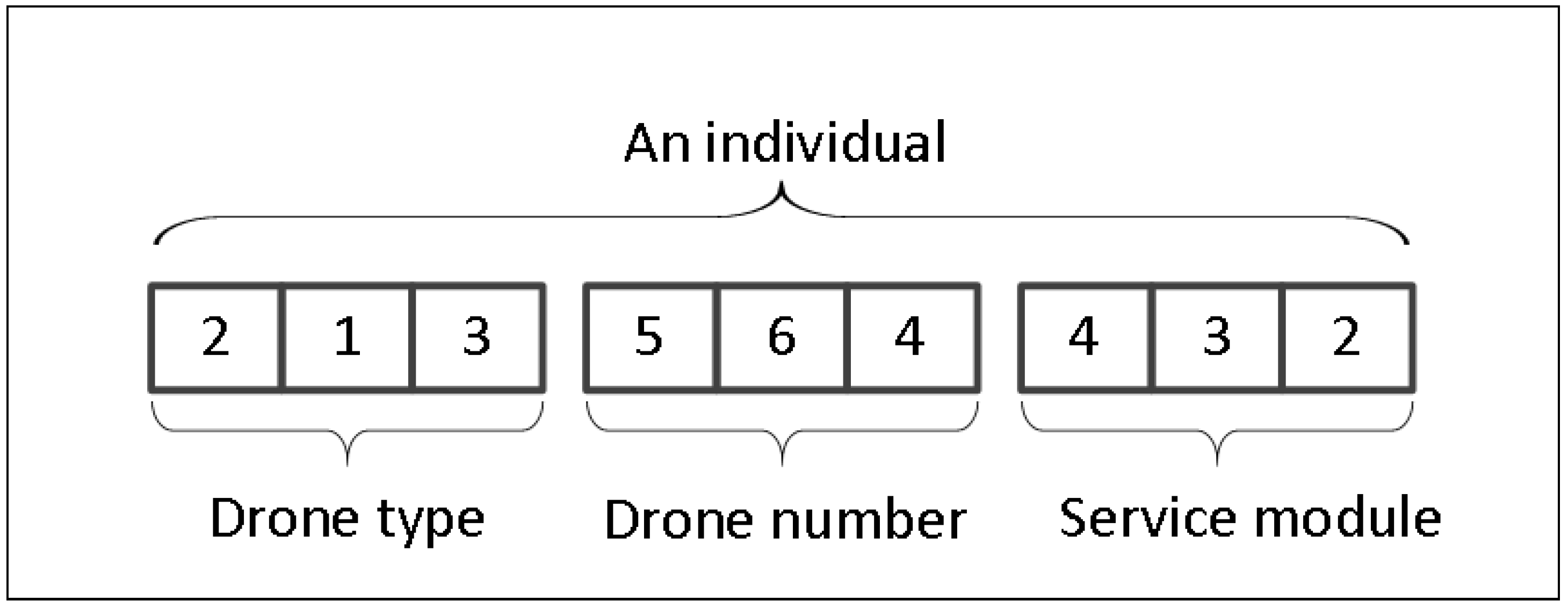
In the developed hybrid GA for the studied stochastic optimization problem, each solution is represented by a chromosome (individual) composed of three parts, as shown in Figure 3, and the three gene parts denote drone type selection, the drone number, and service module: (i) The first part is the selection of drone type on each route, where the number at the rth position denotes the type of drones, (ii) the drone number on each route, and (iii) the drone service module on each route. When the type, number, and service module of drones deployed on each route are determined, under each scenario, parcels of each customer on each route are handled by drones and couriers via a heuristic rule. The heuristic rule is based on the idea that parcels with higher labor cost and smaller volume and weight are delivered by drones. The heuristic rule consists of the following steps: (1) Sort the parcels in decreasing order of $\frac{C_j}{v_j·w_j}$, where j denotes the index of parcels, $C_j$ denotes the labor cost for parcel j delivered by courier, and $v_j$ and $w_j$ denote the volume and weight of parcel j; (2) assign parcels to drones in the obtained sequence with respect to the volume and weight capacities of each drone; and (3) parcels that are not assigned to drones will be delivered by couriers.

For the generation of an initial individual, firstly the type of drones on each route is randomly selected. The drone number and drone service module on each route are randomly generated. If the constraint of Equation (6) is violated for a service route, then the drone number and service module will be regenerated. Since parcels are assigned to drones and couriers via the heuristic rule under each scenario, the sum of drone operating cost and the expectation of the labor cost of couriers can be calculated accordingly.

4.2.2. Crossover and Mutation

During each iteration, offspring solutions are reproduced by current individuals via genetic operators, i.e., the crossover and mutation operations. For the crossover operation, the identical drone types of two parent individuals will be copied to the two offspring solutions. For each service route, if the drone types selected in two parent solutions are the same, then the drone type will be still selected for the route in the offsprings and the corresponding number and service module of drones will be not changed in the offsprings. Otherwise, the type, number, and service module of drones deployed on each route will be reselected randomly for the offsprings. Figure 4 illustrates the crossover procedure. The identical drone types of two parent solutions are labelled with a circle in dotted line, and the type, number, and service of drones on this route are copied to the offspring individuals. Moreover, the type, number, and service module of drones on route 2 and route 3 are randomly generated.

There are two ways for mutation: (1) random modification of the number of drones and (2) random reselection of the service module of drones deployed on each route. The first mutation method is shown in Figure 5; the first mutation method consists of (i) copying the type, number, and service module of drones deployed on each route to the offspring individual; (ii) randomly selecting a service route; and (iii) randomly modifying the number of drones on this route. The second mutation method is illustrated in Figure 6 and includes (i) copying the genetic parts to the offspring solution, (ii) randomly selecting a service route, and (iii) randomly modifying the service module of drones deployed on this route. Then, under each scenario, parcels are assigned to drones and couriers via the heuristic rule.

5. Computational Experiments

In this section, we evaluate the performance of proposed solution approaches by conducting a case study based on the Shanghai Jinshan industrial park network. Both the SAA method and the hybrid GA are coded in MATLAB_2014b, andthe SAA method is combined with CPLEX 12.6. All computational experiments are conducted on a personal computer with a 3.60 GHz processor and 8.00 GB RAM under the Windows 7 operating system. The total computational times of both proposed solution approaches are limited to 3600 s.

For the hybrid GA, a preliminary analysis has been conducted in order to fine-tune the parameters, which are reported in

Table 2. Parameters for hybrid genetic algorithm (GA).

Parameter	Value (Hybrid GA)
Population size	50
Generation number	20
Crossover probability	0.9
Mutation 1 probability	0.2
Mutation 2 probability	0.8

. Population size and maximum iteration number are set to be 50 and 20 respectively.

5.1. Data Generation

We conduct a case study based on the drone delivery information of Ele.me to evaluate the applicability of the proposed solution methods. Ele.me has developed a fleet of drones to delivery food on fixed routes in Shanghai Jinshan industrial park. Based on the transportation and the geographical location information of Shanghai Jinshan industrial park, a network is proposed. The network has a total of 20 customers, as shown in Figure 7. There are 11 service routes, three types of drones, and 4 categories of parcels, as shown in

Table 3. Service routes.

ID	Service Routes
1	Pingan Square → Yunhe Village → Wujiazhai → Zhangjia → Ting South → Pingan Square
2	Pingan Square → Chenjiadai → Dongfeng → Wujiadai →Yuchi → Quanxin → Ting South → Pingan Square
3	Pingan Square → Dongfeng → Xupu Village → Tuanjie → Changlou → Pingan Square
4	Pingan Square → Changlou → Hexing Village → Qiaowan → Pingan Square
5	Pingan Square → Changlou → Fengjiazhai → Hexing Village → Taojiayuan → Qiaowan → Pingan Square
6	Pingan Square → Hexing Village → Wujiazhai → Shijiazhai → Jiangzhunag Village → Pingan Square
7	Pingan Square → Zhangjia → Wujiazhai → Yunhe Village → Fengjiazhai → Changlou → Dongfeng → Chenjiadai → Pingan Square
8	Pingan Square → Ting South → Wujiadai → Xupu Village → Tuanjie → Hexing Village → Qiaowan → Pingan Square
9	Pingan Square → Taojiayuan → Jiangzhuang Village → Yunhe village → Pingan Square
10	Pingan Square → Hexing Village → Wujiazhai → Shijiazhai → Tuanjie → Changlou → Pingan Square
11	Pingan Square → Xupu Village → Wujiadai → Yuchi → Quanxin → Chejiadai → Pingan Square

,

Table 4. Drone types.

Drone Type	Capacity
	Volume (m${}^3$)	Weight (kg)	Operating Cost (Yuan)	Average Speed (km/h)
1	1	30	350	20
2	2	35	420	30
3	3	40	490	40

and

Table 5. Parcel categories.

Parcel Category	Volume (m${}^3$)	Weight (kg)	Labor Cost Per Parcel Per Kilometer (Yuan)
1	0.01	1	0.2
2	0.02	2	0.4
3	0.01	2	0.3
4	0.02	1	0.3

, respectively. Note that the total travel time on each route depends on the drone speed and the total route distance. The planning time period is set to be one week, i.e., 168 h (10,080 min). There are 4 service modules for drones with departure time intervals, i.e., 5, 10, 15 and 20 min with corresponding service frequencies calculated as $f_k=\frac{10080}{t_k^{int}},\forall k\in \mathcal{K}$. The labor cost for a courier delivering a parcel on each leg of each route depends on the distance of the leg. Moreover, we assume the total number of scenarios to be 50. Under each scenario, the number of parcels of each category on each leg of each route per minute is uniformly generated from 1 to 3.

5.2. Computational Results

The computational experiments are conducted and reported in this part. For the two solution methods, after the drone fleet deployment is determined, the objective value is calculated as the sum of the drone leasing and operating costs and the expected labor cost (under all 50 scenarios). Note that the scenario set $\mathsf{\Omega }$ comprises 50 scenarios and that we evaluate the objective value based on the entire $\mathsf{\Omega }$.

An illustrative example based on a small network is first studied to compare the proposed two solution method with the deterministic situation. Note that the deterministic situation is considered where the demand ${\xi }_{ri}^h$ is fixed and equal to its mean value. In the example, there are 6 customers and 3 drone routes, ${\mathcal{I}}_1=[1,2,6,5,1,2,1]$, ${\mathcal{I}}_2=[1,2,3,2,1]$, and ${\mathcal{I}}_3=[2,4,1,2]$. The computational results are reported in

Table 6. An illustrative example.

Route	Deterministic Situation		SAA		HGA
	${\mathit{N}}_{\mathit{drone}}$	Service module	${\mathit{N}}_{\mathit{drone}}$	Service Module	${\mathit{N}}_{\mathit{drone}}$	Service Module
1	2	2	4	1	4	1
2	2	2	3	1	3	1
3	2	2	3	1	3	1
Obj	5003		4900		4987

, where $N_{drone}$ denotes the number of drones deployed in total. Note that drones selected by the three methods are of type 3. We can obtain that the number obtained under the deterministic situation is 5003, which is 103 and 16 larger than those obtained by the SAA and the HGA. That is, considering the uncertain demand is realistic and cost-saving.

The performance of the proposed solution methods under different number of scenarios is tested, and the results are reported in

Table 7. Impact of the number of scenarios $\left|\mathsf{\Omega }\right|$.

$\left|\mathsf{\Omega }\right|$	SAA			HGA
	${\mathit{N}}_{\mathit{drone}}$	Obj ($\times {10}^5$)	Time (s)	${\mathit{N}}_{\mathit{drone}}$	Obj ($\times {10}^5$)	Time (s)
3	50	7.3531	56.0	50	7.5165	48.2
5	50	6.3544	119.3	50	6.3795	66.9
10	50	6.8960	462.7	50	7.0713	79.8
15	50	6.9026	2883.2	50	6.9867	89.5
20	50	7.1125	3600.0	50	7.1602	112.4
25	-	-	-	50	7.0799	138.6
30	-	-	-	50	7.0001	164.2
35	-	-	-	50	6.9762	189.4
40	-	-	-	50	6.8648	249.8
50	-	-	-	50	6.8782	308.7
Average	50	6.9237	1424.2	50	6.9913	144.8
Lower bound	50	6.3544	56.0	50	6.3795	48.2
Upper bound	50	7.3531	3600.0	50	7.5165	308.7

. Scenarios for the solution methods are randomly selected from the given 50 scenarios. The number of scenarios for the solution methods range from 3 to 50. From Table 7, we observe that the SAA obtains a similar objective with the deterministic situation. Moreover, it can be obtained that the computational time of SAA increases dramatically with the number of scenarios and that SAA loses its power to solve the problem within 3600 s if there are 25 scenarios. That is because, when the number of scenarios increases, the number of decision variables and constraints increase rapidly. The average computational time of SAA is 1424.2 s, which is about 9 times larger than that of the hybrid GA. Besides, as the scale of the tested instance is not large, the drone deployment decisions obtained by SAA and the hybrid GA are very similar. The average objective value of the hybrid GA is $6.9913\times {10}^5$, which is about 0.98% larger than that of SAA. In summary, (i) for each test, the quality of solutions obtained by SAA and the hybrid GA is very similar, (ii) SAA is relatively time-consuming and the computational time of SAA increases rapidly with the number of scenarios, and (iii) the average computational time of the hybrid GA is quite smaller than that of SAA.

The impact of the total flight time of drones on each route is examined and reported in

Table 8. The impact of the total flight time of drones on each route.

Increase of the	SAA with 10 Scenarios			HGA with 50 Scenarios
Average Drone Speed	${\mathit{N}}_{\mathit{drone}}$	Time (s)	Obj($\times {10}^5$)	${\mathit{N}}_{\mathit{drone}}$	Time (s)	Obj($\times {10}^5$)
0	50	463.2	6.8960	50	312.7	6.8782
5	44	465.3	6.2485	44	306.3	6.8488
10	42	468.9	6.1849	42	317.9	6.8390
15	39	472.1	6.2458	39	317.2	6.8243
20	35	471.6	6.2346	36	318.3	6.8047
25	34	465.8	6.1793	34	306.6	6.7998
30	30	466.9	6.1345	31	309.9	6.7802
Average	39.1	467.7	6.3034	39.4	312.7	6.8250

. Since the flight time of a drone on each route depends on the distance and the average speed, the increase of average drone speed is set from 0, 5, 10, …, 30 km/h. Based on the analysis on the tradeoff between the solution quality and the computational time, the number of scenarios for SAA is set to be 10 and that for the hybrid GA is set to be 50. For SAA, 10 distinct scenarios are randomly generated from $\mathsf{\Omega }$. After the first-stage decisions, i.e., the drone fleet deployment and drone service module, are determined, the expected labor cost is calculated as the sample average of the labor costs under 50 scenarios. From Table 8, it can be obtained that the number of drones deployed and the objective values decrease when the average speed increases. That may be because, when the average drone speed increases, the total flight time of a drone on each route decreases and the number of drones deployed on each route may decrease in ensuring the constraint of Equation (9). Therefore, the drone operating cost decreases accordingly. Besides, the average computational times of SAA and the hybrid GA are 467.7 and 312.7 seconds, respectively.

The impact of the volume and weight capacities of drones are tested and presented in

Table 9. The impact of the volume and weight capacities of drones.

Increase of Volume	SAA with 10 Scenarios			HGA with 50 Scenarios
and Weight Capacities	${\mathit{N}}_{\mathit{drone}}$	Time (s)	Obj($\times {10}^5$)	${\mathit{N}}_{\mathit{drone}}$	Time (s)	Obj($\times {10}^5$)
(0, 0)	50	467.5	6.8960	50	313.3	6.8782
(0.5, 5)	37	472.6	6.7510	37	311.0	6.8145
(0.5, 10)	37	468.9	6.2560	37	309.8	6.8145
(1, 5)	37	469.8	6.2346	36	320.4	6.8047
(1, 10)	37	470.6	6.1793	37	322.7	6.7998
Average	39.6	469.9	6.4634	39.4	315.4	6.8223

. We increase the volume and weight capacities by four combinations, i.e., (0.5, 5), (0.5, 10), (1, 5), and (1, 10). It can be observed that the number of drones deployed decreases when the volume and weight capacities increase. That may be because, when the capacities increases, the number of parcels can be delivered by a drone increases and thus the time interval may increase. Therefore, the number of drones deployed may decrease in ensuring the constraint of Equation (9) and the objective value may decrease accordingly, as shown in Table 9.

The sensitivity of the value of time intervals $t_k^{int}$ of each service module is then tested. We reduce the time interval of each service module by 1, 2, 3, and 4, respectively. It can be observed from

Table 10. The impact of time interval values.

Decrease of	SAA with 10 Scenarios			HGA with 50 Scenarios
Time Intervals	${\mathit{N}}_{\mathit{drone}}$	Time (s)	Obj($\times {10}^5$)	${\mathit{N}}_{\mathit{drone}}$	Time (s)	Obj($\times {10}^5$)
0	50	466.1	6.8960	50	314.6	6.8782
1	62	464.2	2.4349	62	310.4	2.9725
2	81	478.1	0.9162	81	313.4	1.2973
3	117	472.9	0.5733	117	319.5	0.5769
4	229	469.8	1.1221	228	320.3	1.1221
Average	107.8	470.22	2.3885	107.6	315.6	2.5694

that, when the time interval values decrease, the number of drones deployed increases. That may be because, when the time intervals decrease, the number of drones deployed increases to guarantee the constraint of Equation (9), the number of parcels delivered by drones decreases, and thus the number of parcels handled by couriers decreases. With the decrease of the time intervals, the objective value first decreases and then increases. That may be because there is a tradeoff between the number of drones deployed and the labor cost; when the number of drones on each route is too large, the drone operating cost increases rapidly.

In summary, from the computational results reported in Table 6, Table 7, Table 8, Table 9 and Table 10, it can be obtained that

(1)

with the increase of the number of scenarios, the computational time of SAA increases dramatically;

(2)

given the same number of scenarios, the computational time of the hybrid GA is smaller than SAA with high solution quality;

(3)

with the increase of average drone speed and the total flight time, the number of drones deployed and the total cost decrease;

(4)

when the volume and weight capacities of drones increase, the number of drones deployed and the total cost decrease;

(5)

when the time intervals decrease, the number of drones deployed increases; and

(6)

the developed hybrid GA outperforms the SAA in terms of the computational time with high solution quality.

Therefore, for the stochastic drone fleet deployment and planning problem in multiple-type parcel delivery service, we recommend applying SAA when the number of scenarios is small and applying the hybrid GA method when the number of scenarios is large.

6. Conclusions

This work studies the stochastic drone fleet deployment and planning problem in multiple-type parcel delivery service. In the problem, the drone fleet deployment, i.e., the type, number, and service module of drones deployed on each route, should be decided with uncertain parcel demand. Under each realized scenario, the number of parcels delivered by drones and couriers should be determined. The objective is to minimize the sum of the drone leasing and operating costs and the expected labor cost. A novel two-stage stochastic programming formulation is proposed. To solve the problem, a classic SAA is applied and a hybrid GA is further developed to achieve computational efficiency.

Future research directions may include (i) designing heuristics that can solve the problem more efficiently; (ii) considering more practical conditions, such as the situation where the labor cost function is more complicated; (iii) considering heterogeneous drones on each drone route; and (iv) studying the problem with labor cost as a piecewise or convex function.

References

- Sikeridis, D.; Tsiropoulou, E.E.; Devetsikiotis, M.; Papavassiliou, S. Wireless powered Public Safety IoT: A UAV-assisted adaptive-learning approach towards energy efficiency. J. Netw. Comput. Appl. 2018, 123, 69–79. [Google Scholar] [CrossRef]
- Hong, I.; Kuby, M.; Murray, A.T. A range-restricted recharging station coverage model for drone delivery service planning. Transp. Res. Part Emerg. Technol. 2018, 90, 198–212. [Google Scholar] [CrossRef]
- Zhang, C.; Kovacs, J.M. The application of small unmanned aerial systems for precision agriculture: A review. Precis. Agric. 2012, 13, 693–712. [Google Scholar] [CrossRef]
- Aleem, Z. The Chinese Version of Amazon Is Already Using Drones to Deliver Stuff to Customers; Vox Media, Inc.: New York, NY, USA, 2017. [Google Scholar]
- Rose, C. Amazon’s Jeff Bezos looks to the future. CBS News, 1 December 2013. [Google Scholar]
- Hu, Y. Your takeaway order in Shanghai might soon be delivered by a drone. Urban Family, 31 May 2018. [Google Scholar]
- Pymnts. Ele.me Clared to Use Food Delivery Drones in China. 2018. Available online: https://www.pymnts.com/news/delivery/2018/eleme-food-delivery-drones-china/ (accessed on 31 May 2018).
- Scott, J.; Scott, C. Drone delivery models for healthcare. In Proceedings of the 50th Hawaii International Conference on System Sciences, Waikoloa Village, HI, USA, 4–7 January 2017. [Google Scholar] [CrossRef]
- Shavarani, S.M.; Nejad, M.G.; Rismanchian, F.; Izbirak, G. Application of hierarchical facility location problem for optimization of a drone delivery system: a case study of Amazon prime air in the city of San Francisco. Int. J. Adv. Manuf. Technol. 2018, 95, 3141–3153. [Google Scholar] [CrossRef]
- Murray, C.C.; Chu, A.G. The flying sidekick traveling salesman problem: Optimization of drone-assisted parcel delivery. Transp. Res. Part Emerg. Technol. 2015, 54, 86–109. [Google Scholar] [CrossRef]
- Chow, J.Y. Dynamic UAV-based traffic monitoring under uncertainty as a stochastic arc-inventory routing policy. Int. J. Transp. Sci. Technol. 2016, 5, 167–185. [Google Scholar] [CrossRef]
- Tavana, M.; Khalili-Damghani, K.; Santos-Arteaga, F.J.; Zandi, M.H. Drone shipping versus truck delivery in a cross-docking system with multiple fleets and products. Expert Syst. Appl. 2017, 72, 93–107. [Google Scholar] [CrossRef]
- Dorling, K.; Heinrichs, J.; Messier, G.G.; Magierowski, S. Vehicle routing problems for drone delivery. IEEE Trans. Syst. Man Cybern. Syst. 2016, 47, 70–85. [Google Scholar] [CrossRef]
- Furini, F.; Persiani, C.A.; Toth, P. The time dependent traveling salesman planning problem in controlled airspace. Transp. Res. Part Methodol. 2016, 90, 38–55. [Google Scholar] [CrossRef]
- Keeney. How Can Amazon Charge $1 for Drone Delivery. 2015. Available online: https://ark-invest.com/research/drone-delivery-amazon (accessed on 5 May 2015).
- Perdikaki, O.; Kostamis, D.; Swaminathan, J.M. Timing of service investments for retailers under competition and demand uncertainty. Eur. J. Oper. Res. 2016, 254, 188–201. [Google Scholar] [CrossRef]
- Birge, J.R.; Louveaux, F. Introduction to Stochastic Programming; Springer: New York, NY, USA, 2011. [Google Scholar]
- Liu, M.; Liu, X.; Zhang, E.; Chu, F.; Chu, C. Scenario-based heuristic to two-stage stochastic program for the parallel machine ScheLoc problem. Int. J. Prod. Res. 2019, 57, 1706–1723. [Google Scholar] [CrossRef]
- Francis, P.; Smilowitz, K.; Tzur, M. The period vehicle routing problem with service choice. Transp. Sci. 2006, 40, 439–454. [Google Scholar] [CrossRef]
- Guenard, N.; Hamel, T.; Mahony, R. A practical visual servo control for an unmanned aerial vehicle. IEEE Trans. Robot. 2008, 24, 331–340. [Google Scholar] [CrossRef]
- McGonigle, A.; Aiuppa, A.; Giudice, G.; Tamburello, G.; Hodson, A.; Gurrieri, S. Unmanned aerial vehicle measurements of volcanic carbon dioxide fluxes. Geophys. Res. Lett. 2008, 35. [Google Scholar] [CrossRef] [Green Version]
- Dunford, R.; Michel, K.; Gagnage, M.; Piégay, H.; Trémelo, M.L. Potential and constraints of Unmanned Aerial Vehicle technology for the characterization of Mediterranean riparian forest. Int. J. Remote Sens. 2009, 30, 4915–4935. [Google Scholar] [CrossRef]
- Baluja, J.; Diago, M.P.; Balda, P.; Zorer, R.; Meggio, F.; Morales, F.; Tardaguila, J. Assessment of vineyard water status variability by thermal and multispectral imagery using an unmanned aerial vehicle (UAV). Irrig. Sci. 2012, 30, 511–522. [Google Scholar] [CrossRef]
- Herissé, B.; Hamel, T.; Mahony, R.; Russotto, F.X. Landing a VTOL unmanned aerial vehicle on a moving platform using optical flow. IEEE Trans. Robot. 2011, 28, 77–89. [Google Scholar] [CrossRef]
- Mozaffari, M.; Saad, W.; Bennis, M.; Debbah, M. Unmanned aerial vehicle with underlaid device-to-device communications: Performance and tradeoffs. IEEE Trans. Wirel. Commun. 2016, 15, 3949–3963. [Google Scholar] [CrossRef]
- Ulmer, M.W.; Thomas, B.W. Same-day delivery with heterogeneous fleets of drones and vehicles. Networks 2018, 72, 475–505. [Google Scholar] [CrossRef]
- Campbell, J.F.; Sweeney, D.; Zhang, J. Strategic Design for Delivery with Trucks and Drones; Supply Chain Analytics Report SCMA; SCMA-2017-0201; University of Missouri-St. Louis: St. Louis, MO, USA, 2017. [Google Scholar]
- Agatz, N.; Bouman, P.; Schmidt, M. Optimization approaches for the traveling salesman problem with drone. Transp. Sci. 2018, 52, 965–981. [Google Scholar] [CrossRef]
- Venkatachalam, S.; Sundar, K.; Rathinam, S. Two-stage stochastic programming model for routing multiple drones with fuel constraints. arXiv 2017, arXiv:1711.04936. [Google Scholar]
- Mozaffari, M.; Saad, W.; Bennis, M.; Debbah, M. Mobile unmanned aerial vehicles (UAVs) for energy-efficient internet of things communications. IEEE Trans. Wirel. Commun. 2017, 16, 7574–7589. [Google Scholar] [CrossRef]
- Sikeridis, D.; EleniTsiropoulou, E.; Devetsikiotis, M.; Papavassiliou, S. Self-Adaptive Energy Efficient Operation in UAV-Assisted Public Safety Networks. In Proceedings of the 2018 IEEE 19th International Workshop on Signal Processing Advances in Wireless Communications (SPAWC), Kalamata, Greece, 25–28 June 2018; pp. 1–5. [Google Scholar]
- Wang, S.; Meng, Q. Liner ship route schedule design with sea contingency time and port time uncertainty. Transp. Res. Part B 2012, 46, 615–633. [Google Scholar] [CrossRef]
- Meng, Q.; Wang, S. Liner ship fleet deployment with week-dependent container shipment demand. Eur. J. Oper. Res. 2012, 222, 241–252. [Google Scholar] [CrossRef]
- Wang, S.; Meng, Q. Robust bunker management for liner shipping networks. Eur. J. Oper. Res. 2015, 243, 789–797. [Google Scholar] [CrossRef]
- Kleywegt, A.J.; Nori, V.S.; Savelsbergh, M.W.P. The Stochastic Inventory Routing Problem with Direct Deliveries. Transp. Sci. 2002, 36, 94–118. [Google Scholar] [CrossRef] [Green Version]
- Pagnoncelli, B.K.; Ahmed, S.; Shapiro, A. Sample Average Approximation Method for Chance Constrained Programming: Theory and Applications. J. Optim. Theory Appl. 2009, 142, 399–416. [Google Scholar] [CrossRef] [Green Version]
- Ralph, D.; Xu, H. Convergence of stationary points of sample average two-stage stochastic programs: A generalized equation approach. Math. Oper. Res. 2011, 36, 568–592. [Google Scholar] [CrossRef]
- Verweij, B.; Ahmed, S.; Kleywegt, A.J.; Nemhauser, G.; Shapiro, A. The sample average approximation method applied to stochastic routing problems: a computational study. Comput. Optim. Appl. 2003, 24, 289–333. [Google Scholar] [CrossRef]
- Wang, W.; Ahmed, S. Sample average approximation of expected value constrained stochastic programs. Oper. Res. Lett. 2008, 36, 515–519. [Google Scholar] [CrossRef]
- Bertsimas, D.; Gupta, V.; Kallus, N. Robust sample average approximation. Math. Program. 2017, 171, 217–282. [Google Scholar] [CrossRef] [Green Version]
- Kalayci, C.B.; Polat, O.; Gupta, S.M. A hybrid genetic algorithm for sequence-dependent disassembly line balancing problem. Ann. Oper. Res. 2016, 242, 321–354. [Google Scholar] [CrossRef]
- Holland, J.H. Adaptation in natural and artificial systems. Q. Rev. Biol. 1975, 6, 126–137. [Google Scholar]
Figure 1.
An illustrative example.
Figure 2.
An illustrative example for service module.
Figure 3.
Coding (parcels are assigned to drones and couriers via the heuristic rule).
Figure 4.
Crossover (reproducing the identical genetic parts between parents to offsprings).
Figure 5.
Mutation 1 (random modification of drone numbers).
Figure 6.
Mutation 2 (random modification of drone service modules).
Figure 7.
Shanghai Jinshan industrial park drone delivery network.